A data-driven examination of how Norwegian industrial production, residential construction by dwelling type, and labour force participation by age group have moved in divergent directions in recent years.
Published
September 21, 2026
Norway’s economy has long defied simple characterisation. Petroleum wealth underwrites the sovereign fund, mainland industry competes under a strong currency, construction cycles feed and frustrate housing affordability, and a rapidly ageing population reshapes who actually shows up for work. Three datasets from Statistics Norway allow us to probe these tensions simultaneously — sectoral gross output, new dwelling construction by type, and labour force status by age group — and the combined picture is more nuanced than either optimists or pessimists typically acknowledge.
# ---- df1 wrangling: sectoral gross value added at current prices ----df1_gva <-NULLdf1_gva_wide <-NULLdf1_lollipop <-NULLif (!is.null(df1) &&nrow(df1) >0) { target_measure <-"Bruttoprodukt i basisverdi. Løpende priser (mill. kr)" target_sectors <-c("Totalt for næringer","Jordbruk og skogbruk","Industri","Utvinning av råolje og naturgass, inkl. tjenester" ) df1_gva <- df1 |>filter( .data[["statistikkvariabel"]] == target_measure, .data[["næring"]] %in% target_sectors )if (nrow(df1_gva) ==0) {message("df1_gva empty. Measures: ",paste(head(unique(df1[["statistikkvariabel"]]), 8), collapse =" | "))message("Sectors: ",paste(head(unique(df1[["næring"]]), 8), collapse =" | ")) df1_gva <-NULL }if (!is.null(df1_gva)) {# Lollipop: latest-year GVA level per sector (excl. total) max_year <-max(df1_gva$date) df1_lollipop <- df1_gva |>filter(date == max_year, næring !="Totalt for næringer") |>mutate(sector_label = næring,value_bn = value /1000) # convert mill. kr -> mrd. kr }}# ---- df2 wrangling: dwellings completed by type, national total ----df2_national <-NULLdf2_area <-NULLdf2_share <-NULLdf2_latest <-NULLif (!is.null(df2) &&nrow(df2) >0) {# "region" column will be present; aggregate nationally region_col_name <-names(df2)[names(df2) %in%c("region", "Region")]if (length(region_col_name) ==0) region_col_name <-NULL dwelling_types <-c("Enebolig","Tomannsbolig","Rekkehus, kjedehus og andre småhus","Boligblokk","Bygning for bofellesskap" ) df2_national <- df2 |>filter(.data[["bygningstype"]] %in% dwelling_types) |>group_by(date, time_str, bygningstype) |>summarise(value =sum(value, na.rm =TRUE), .groups ="drop")if (nrow(df2_national) ==0) {message("df2_national empty. Types: ",paste(head(unique(df2[["bygningstype"]]), 8), collapse =" | ")) df2_national <-NULL }if (!is.null(df2_national)) {# Area chart data df2_area <- df2_national |>mutate(type_label =case_when( bygningstype =="Enebolig"~"Detached", bygningstype =="Tomannsbolig"~"Semi-detached", bygningstype =="Rekkehus, kjedehus og andre småhus"~"Terraced / small", bygningstype =="Boligblokk"~"Apartment block", bygningstype =="Bygning for bofellesskap"~"Communal dwelling",TRUE~ bygningstype ))# Share of each type in latest year latest_yr <-max(df2_area$date) total_latest <- df2_area |>filter(date == latest_yr) |>summarise(tot =sum(value)) |>pull(tot) df2_latest <- df2_area |>filter(date == latest_yr) |>mutate(share = value / total_latest *100) |>arrange(desc(share)) }}# ---- df3 wrangling: employed persons by age group ----df3_employed <-NULLdf3_outside <-NULLdf3_dumbbell <-NULLdf3_ridgeline <-NULLif (!is.null(df3) &&nrow(df3) >0) { age_groups <-c("15-24 år", "25-54 år", "55-74 år") sex_col <-names(df3)[names(df3) %in%c("kjønn", "kjonn", "Kjønn", "Kjonn")]if (length(sex_col) ==0) sex_col <-NULL# Employed (total both sexes) df3_employed <- df3 |>filter( .data[["arbeidsstyrkestatus"]] =="Sysselsatte", .data[["alder"]] %in% age_groups )if (!is.null(sex_col) &&length(sex_col) >0) { sex_vals <-unique(df3[[sex_col[1]]]) both_val <- sex_vals[grepl("begge|i alt|total|both", sex_vals, ignore.case =TRUE)]if (length(both_val) >0) { df3_employed <- df3_employed |>filter(.data[[sex_col[1]]] == both_val[1]) } }if (nrow(df3_employed) ==0) {message("df3_employed empty. Status: ",paste(head(unique(df3[["arbeidsstyrkestatus"]]), 8), collapse =" | ")) df3_employed <-NULL }# Outside labour force (55-74 yr focus) df3_outside <- df3 |>filter( .data[["arbeidsstyrkestatus"]] =="Personer utenfor arbeidsstyrken", .data[["alder"]] %in% age_groups )if (!is.null(sex_col) &&length(sex_col) >0) { sex_vals <-unique(df3[[sex_col[1]]]) both_val <- sex_vals[grepl("begge|i alt|total|both", sex_vals, ignore.case =TRUE)]if (length(both_val) >0) { df3_outside <- df3_outside |>filter(.data[[sex_col[1]]] == both_val[1]) } }if (nrow(df3_outside) ==0) { df3_outside <-NULL }# Dumbbell: earliest vs latest year, employed by age groupif (!is.null(df3_employed) &&nrow(df3_employed) >0) { yr_min <-min(df3_employed$date) yr_max <-max(df3_employed$date) df3_dumbbell <- df3_employed |>filter(date %in%c(yr_min, yr_max)) |>mutate(period =if_else(date == yr_min, "Earliest", "Latest")) |>select(alder, period, value) |>pivot_wider(names_from = period, values_from = value) |>filter(!is.na(Earliest), !is.na(Latest)) |>mutate(change =as.numeric(Latest) -as.numeric(Earliest)) # fixed: ensure numeric subtraction }# Ridgeline prep: employed across years, by age groupif (!is.null(df3_employed) &&nrow(df3_employed) >0) { df3_ridgeline <- df3_employed |>mutate(year_num =as.numeric(format(date, "%Y"))) }}
Error in `mutate()`:
ℹ In argument: `change = as.numeric(Latest) - as.numeric(Earliest)`.
Caused by error:
! 'list' object cannot be coerced to type 'double'
Sectoral Gross Value Added: Oil vs. Industry vs. Agriculture
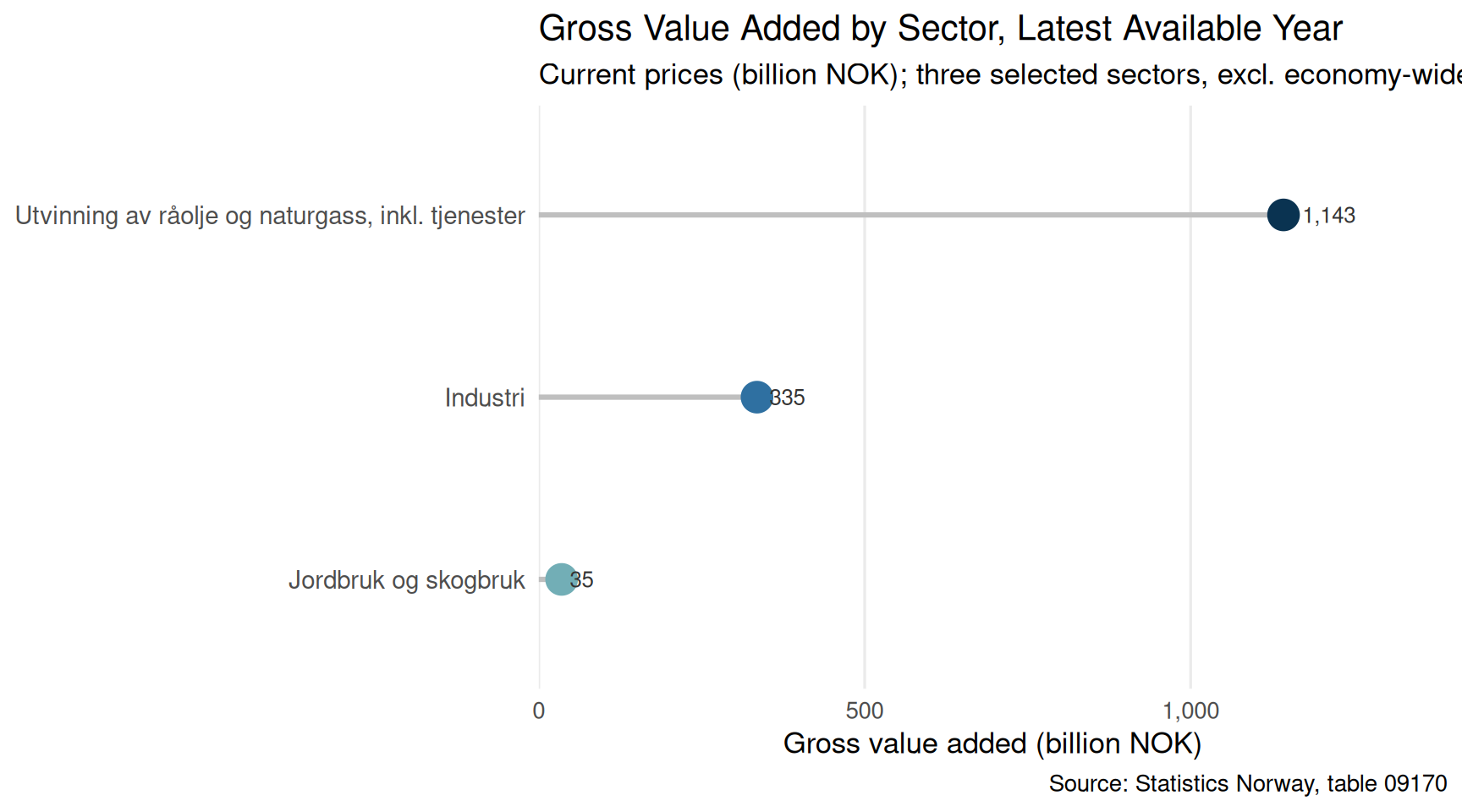
Norway’s three headline production sectors could hardly be more different in scale and trajectory. Petroleum extraction, mainland manufacturing, and agriculture each respond to entirely different forces — commodity price cycles, global demand, weather — yet they are all tallied in the same national accounts. The chart below puts their gross value added (GVA) in current prices side by side, stripping away the economy-wide total to focus on the sectoral contrasts.
Code
if (exists("df1_lollipop") &&!is.null(df1_lollipop) &&nrow(df1_lollipop) >0) { pal <- MetBrewer::met.brewer("Hokusai2", n =nrow(df1_lollipop)) p <-ggplot(df1_lollipop,aes(x = value_bn,y =reorder(sector_label, value_bn),colour =reorder(sector_label, value_bn))) +geom_segment(aes(x =0, xend = value_bn,yend =reorder(sector_label, value_bn)),linewidth =1.1, colour ="grey75") +geom_point(size =6) +geom_text(aes(label = scales::comma(round(value_bn, 0))),hjust =-0.35, size =3.4, colour ="grey20") +scale_colour_manual(values = pal, guide ="none") +scale_x_continuous(labels = scales::comma,expand =expansion(mult =c(0, 0.22))) +labs(title ="Gross Value Added by Sector, Latest Available Year",subtitle ="Current prices (billion NOK); three selected sectors, excl. economy-wide total",x ="Gross value added (billion NOK)",y =NULL,caption ="Source: Statistics Norway, table 09170" ) +theme_minimal(base_size =13) +theme(panel.grid.major.y =element_blank(),panel.grid.minor =element_blank(),axis.text.y =element_text(size =11) )print(p) top_sec <- df1_lollipop[which.max(df1_lollipop$value_bn), ] low_sec <- df1_lollipop[which.min(df1_lollipop$value_bn), ] yr_label <-format(max(df1_lollipop$date), "%Y")cat(sprintf("\nIn %s, **%s** recorded the largest gross value added among the three sectors at %.0f billion NOK, while **%s** posted the smallest at %.0f billion NOK — a ratio of roughly %.0f-to-one.\n\n", yr_label, top_sec$sector_label, top_sec$value_bn, low_sec$sector_label, low_sec$value_bn, top_sec$value_bn / low_sec$value_bn ))} else {cat("\n*Figure omitted — Statistics Norway returned no data for this series.*\n\n")}
In 2025, **Utvinning av råolje og naturgass, inkl. tjenester** recorded the largest gross value added among the three sectors at 1143 billion NOK, while **Jordbruk og skogbruk** posted the smallest at 35 billion NOK — a ratio of roughly 33-to-one.
Code
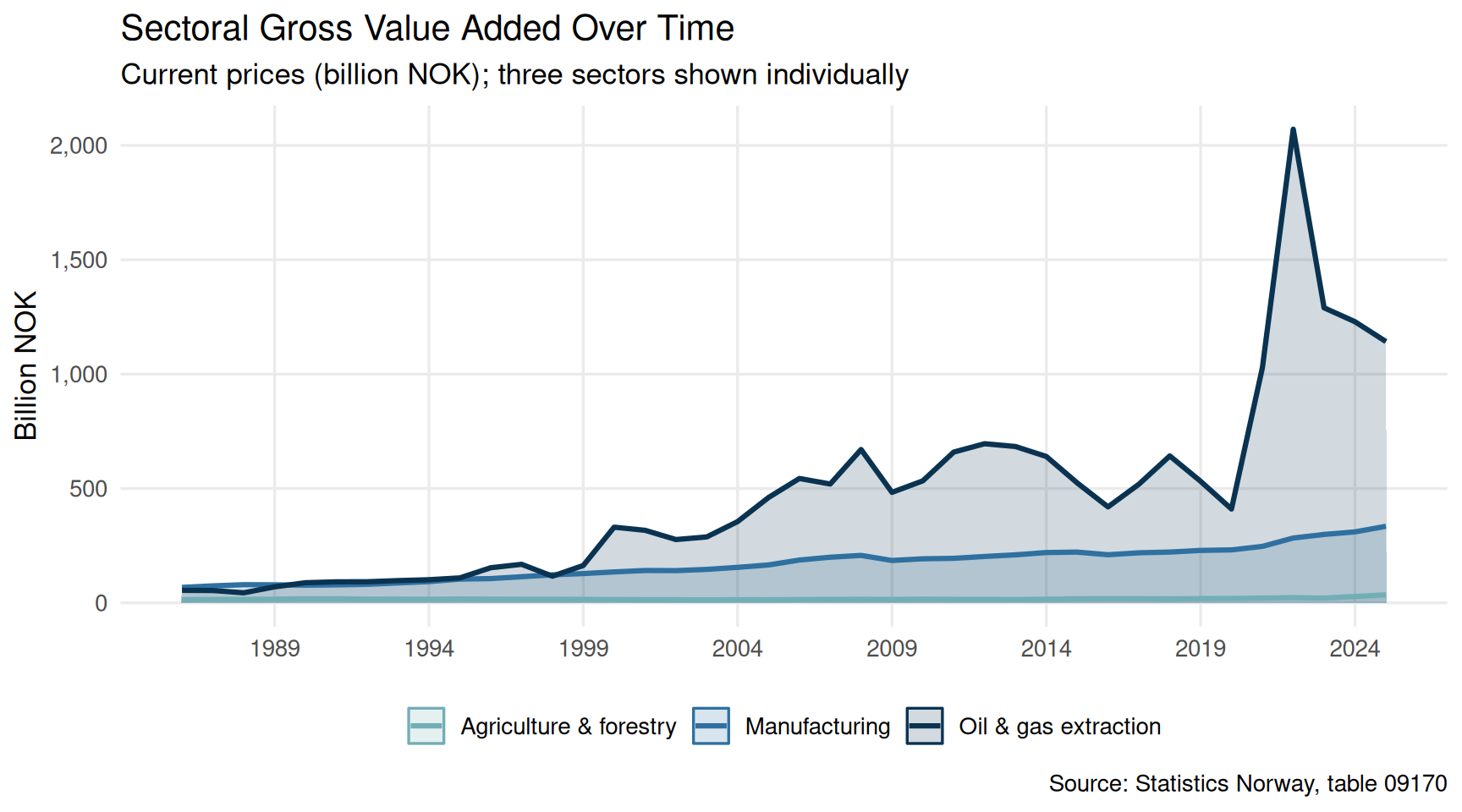
if (exists("df1_gva") &&!is.null(df1_gva) &&nrow(df1_gva) >0) { df1_area_plot <- df1_gva |>filter(næring !="Totalt for næringer") |>mutate(sector_label =case_when( næring =="Jordbruk og skogbruk"~"Agriculture & forestry", næring =="Industri"~"Manufacturing", næring =="Utvinning av råolje og naturgass, inkl. tjenester"~"Oil & gas extraction",TRUE~ næring ),value_bn = value /1000 )if (nrow(df1_area_plot) >0) { pal3 <- MetBrewer::met.brewer("Hokusai2", n =3) p2 <-ggplot(df1_area_plot,aes(x = date, y = value_bn,colour = sector_label, fill = sector_label)) +geom_area(alpha =0.18, position ="identity") +geom_line(linewidth =1.1) +scale_colour_manual(values = pal3, name =NULL) +scale_fill_manual(values = pal3, name =NULL) +scale_x_date(date_breaks ="5 years", date_labels ="%Y") +scale_y_continuous(labels = scales::comma) +labs(title ="Sectoral Gross Value Added Over Time",subtitle ="Current prices (billion NOK); three sectors shown individually",x =NULL,y ="Billion NOK",caption ="Source: Statistics Norway, table 09170" ) +theme_minimal(base_size =13) +theme(legend.position ="bottom",panel.grid.minor =element_blank() )print(p2)# Compute growth from first to last year per sector first_yr <-min(df1_area_plot$date) last_yr <-max(df1_area_plot$date) growth_tbl <- df1_area_plot |>filter(date %in%c(first_yr, last_yr)) |>select(sector_label, date, value_bn) |>pivot_wider(names_from = date, values_from = value_bn,names_prefix ="yr_") |>mutate(pct_chg = (.data[[paste0("yr_", last_yr)]] / .data[[paste0("yr_", first_yr)]] -1) *100) |>arrange(desc(pct_chg))cat(sprintf("\nBetween %s and %s, **%s** showed the steepest percentage growth in GVA at current prices (+%.0f%%), compared with **%s** which grew by +%.0f%%.\n\n",format(first_yr, "%Y"), format(last_yr, "%Y"), growth_tbl$sector_label[1], growth_tbl$pct_chg[1], growth_tbl$sector_label[nrow(growth_tbl)], growth_tbl$pct_chg[nrow(growth_tbl)] )) } else {cat("\n*Figure omitted — Statistics Norway returned no data for this series.*\n\n") }} else {cat("\n*Figure omitted — Statistics Norway returned no data for this series.*\n\n")}
Between 1986 and 2025, **Oil & gas extraction** showed the steepest percentage growth in GVA at current prices (+1984%), compared with **Agriculture & forestry** which grew by +151%.
Construction: What Norway Is (and Is Not) Building
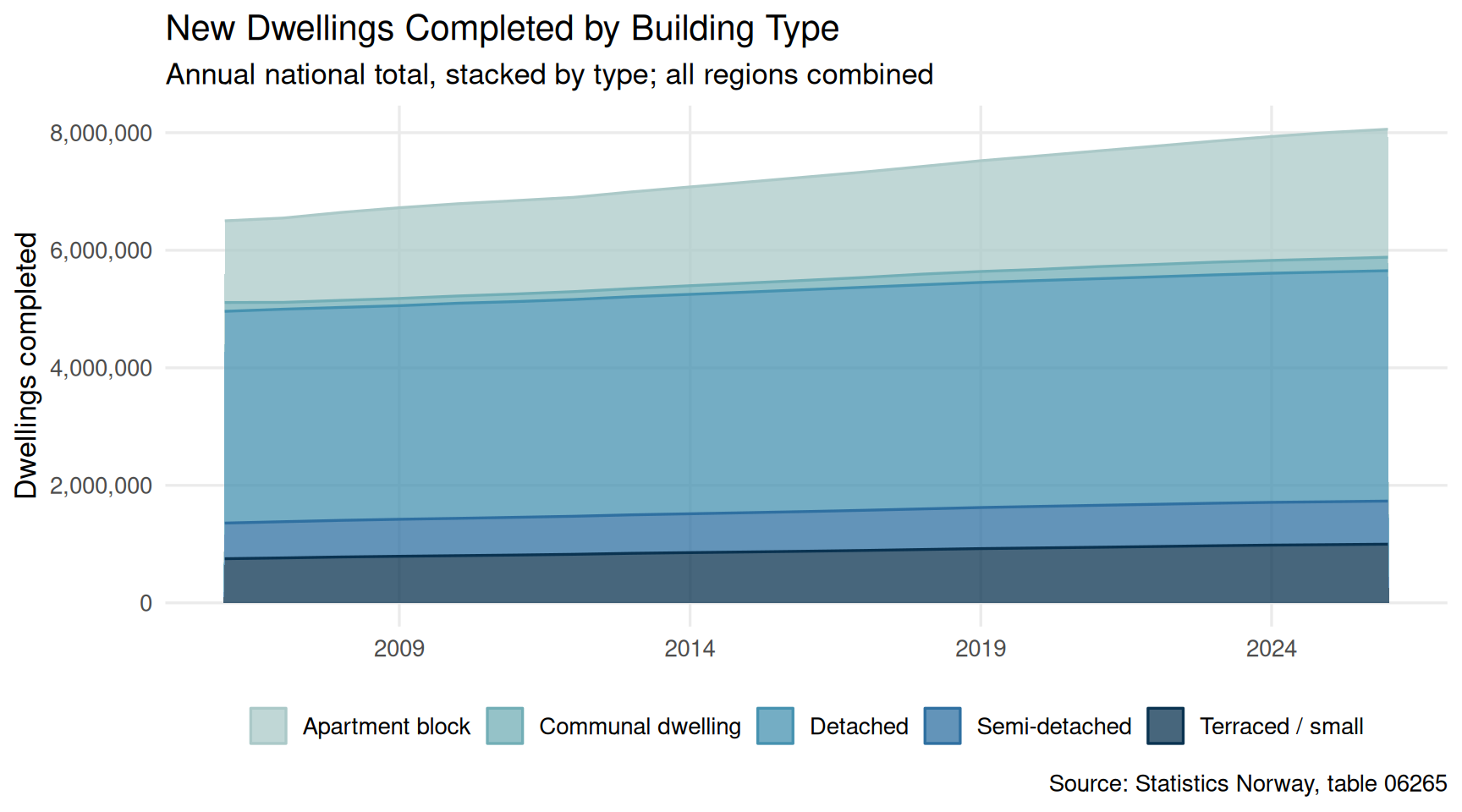
The mix of dwelling types completed each year is a reliable barometer of how developers read demand signals — density pressure in cities, affordability constraints, planning policy, and interest rate sensitivity all leave fingerprints on the composition of new housing supply. A shift from detached houses toward apartment blocks, or vice versa, has long-run consequences for urban form and household formation.
Code
if (exists("df2_area") &&!is.null(df2_area) &&nrow(df2_area) >0) { pal5 <- MetBrewer::met.brewer("Hokusai2", n =5) p3 <-ggplot(df2_area,aes(x = date, y = value,colour = type_label, fill = type_label)) +geom_area(position ="stack", alpha =0.75) +scale_colour_manual(values = pal5, name =NULL) +scale_fill_manual(values = pal5, name =NULL) +scale_x_date(date_breaks ="5 years", date_labels ="%Y") +scale_y_continuous(labels = scales::comma) +labs(title ="New Dwellings Completed by Building Type",subtitle ="Annual national total, stacked by type; all regions combined",x =NULL,y ="Dwellings completed",caption ="Source: Statistics Norway, table 06265" ) +theme_minimal(base_size =13) +theme(legend.position ="bottom",panel.grid.minor =element_blank() )print(p3)if (!is.null(df2_latest) &&nrow(df2_latest) >0) { top_type <- df2_latest[1, ] yr_label <-format(max(df2_area$date), "%Y") total_comp <-sum(df2_latest$value)cat(sprintf("\nIn %s, **%s** was the most common completed dwelling type, accounting for %.1f%% of the %.0f total completions. The smallest share belonged to **%s** (%.1f%%).\n\n", yr_label, top_type$type_label, top_type$share, total_comp, df2_latest$type_label[nrow(df2_latest)], df2_latest$share[nrow(df2_latest)] )) }} else {cat("\n*Figure omitted — Statistics Norway returned no data for this series.*\n\n")}
In 2026, **Detached** was the most common completed dwelling type, accounting for 48.6% of the 8058612 total completions. The smallest share belonged to **Communal dwelling** (2.8%).
Labour Force Participation Across Age Groups
The shape of Norway’s workforce is shifting. An ageing population means that decisions made by those aged 55 to 74 — whether to stay in the labour force or exit — have growing macroeconomic weight. At the same time, youth participation patterns and prime-age employment rates determine productivity and tax base trajectories for decades.
Code
if (exists("df3_dumbbell") &&!is.null(df3_dumbbell) &&nrow(df3_dumbbell) >0) { pal_db <- MetBrewer::met.brewer("Hokusai2", n =2) p4 <-ggplot(df3_dumbbell,aes(y = alder)) +geom_segment(aes(x = Earliest, xend = Latest,yend = alder),linewidth =1.8, colour ="grey70") +geom_point(aes(x = Earliest, colour ="Earliest year"),size =5) +geom_point(aes(x = Latest, colour ="Latest year"),size =5) +geom_text(aes(x = Latest,label =ifelse(change >0,paste0("+", scales::comma(round(change, 0))), scales::comma(round(change, 0)))),hjust =-0.3, size =3.3, colour ="grey25") +scale_colour_manual(values = pal_db, name =NULL) +scale_x_continuous(labels = scales::comma,expand =expansion(mult =c(0.02, 0.18))) +labs(title ="Employed Persons by Age Group: Earliest vs. Latest Year",subtitle ="Both sexes combined; absolute count change shown at right end",x ="Employed persons (thousands or persons — as reported by SSB)",y ="Age group",caption ="Source: Statistics Norway, table 05111" ) +theme_minimal(base_size =13) +theme(legend.position ="bottom",panel.grid.major.y =element_blank(),panel.grid.minor =element_blank() )print(p4) # fixed: added explicit print() to render plot gainers <- df3_dumbbell |>filter(change >0) |>arrange(desc(change)) losers <- df3_dumbbell |>filter(change <0) |>arrange(change) yr_min <-format(min(df3_employed$date), "%Y") yr_max <-format(max(df3_employed$date), "%Y")if (nrow(gainers) >0) {cat(sprintf("\nBetween %s and %s, the **%s** age group recorded the largest absolute gain in employed persons (+%s). ", yr_min, yr_max, gainers$alder[1], scales::comma(round(gainers$change[1], 0)) )) }if (nrow(losers) >0) {cat(sprintf("The **%s** group saw the sharpest decline (%s persons).\n\n", losers$alder[1], scales::comma(round(losers$change[1], 0)) )) } else {cat("\n\n") }} else {cat("\n*Figure omitted — Statistics Norway returned no data for this series.*\n\n")}
*Figure omitted — Statistics Norway returned no data for this series.*
Code
if (exists("df3_ridgeline") &&!is.null(df3_ridgeline) &&nrow(df3_ridgeline) >0) { pal_ridge <- MetBrewer::met.brewer("Hokusai2", n =3) p5 <-ggplot(df3_ridgeline,aes(x = value, y = alder, fill = alder)) + ggridges::geom_density_ridges(alpha =0.72,scale =1.2,rel_min_height =0.01,colour ="white" ) +scale_fill_manual(values = pal_ridge, guide ="none") +scale_x_continuous(labels = scales::comma) +labs(title ="Distribution of Annual Employment Counts by Age Group",subtitle ="Density ridgeline across all available years; both sexes combined",x ="Employed persons (as reported by SSB)",y ="Age group",caption ="Source: Statistics Norway, table 05111" ) +theme_minimal(base_size =13) +theme(panel.grid.minor =element_blank())print(p5) # fixed: added explicit print() to render plot spread_tbl <- df3_ridgeline |>group_by(alder) |>summarise(med =median(value, na.rm =TRUE),spread =sd(value, na.rm =TRUE),.groups ="drop" ) |>arrange(desc(spread))cat(sprintf("\nThe **%s** age group shows the widest year-to-year variation in employment (SD = %s persons), suggesting this cohort is most sensitive to economic cycles. The **%s** group has the narrowest spread (SD = %s persons).\n\n", spread_tbl$alder[1], scales::comma(round(spread_tbl$spread[1], 0)), spread_tbl$alder[nrow(spread_tbl)], scales::comma(round(spread_tbl$spread[nrow(spread_tbl)], 0)) ))} else {cat("\n*Figure omitted — Statistics Norway returned no data for this series.*\n\n")}
*Figure omitted — Statistics Norway returned no data for this series.*
Key Findings
Code
bullets <-character(0)# df1 findingsif (!is.null(df1_lollipop) &&nrow(df1_lollipop) >0) { top_sec <- df1_lollipop[which.max(df1_lollipop$value_bn), ] low_sec <- df1_lollipop[which.min(df1_lollipop$value_bn), ] yr_label <-format(max(df1_lollipop$date), "%Y") bullets <-c(bullets, sprintf("- **Sectoral GVA (%s):** %s leads at %.0f billion NOK; %s registers %.0f billion NOK — a gap of %.0fx.", yr_label, top_sec$sector_label, top_sec$value_bn, low_sec$sector_label, low_sec$value_bn, top_sec$value_bn / low_sec$value_bn ))}# df2 findingsif (!is.null(df2_latest) &&nrow(df2_latest) >0) { top_type <- df2_latest[1, ] total_comp <-sum(df2_latest$value) yr_label <-format(max(df2_area$date), "%Y") bullets <-c(bullets, sprintf("- **Housing completions (%s):** %s was the dominant dwelling type (%.1f%% of %.0f completions); %s was least common (%.1f%%).", yr_label, top_type$type_label, top_type$share, total_comp, df2_latest$type_label[nrow(df2_latest)], df2_latest$share[nrow(df2_latest)] ))}# df3 findingsif (!is.null(df3_dumbbell) &&nrow(df3_dumbbell) >0) { gainers <- df3_dumbbell |>filter(change >0) |>arrange(desc(change)) losers <- df3_dumbbell |>filter(change <0) |>arrange(change) yr_min <-format(min(df3_employed$date), "%Y") yr_max <-format(max(df3_employed$date), "%Y")if (nrow(gainers) >0) { bullets <-c(bullets, sprintf("- **Employment by age (%s–%s):** The %s group gained the most employed persons (+%s), while %s %s.", yr_min, yr_max, gainers$alder[1], scales::comma(round(gainers$change[1], 0)),if (nrow(losers) >0) losers$alder[1] else"no group",if (nrow(losers) >0)sprintf("saw a net decline (%s persons)", scales::comma(round(losers$change[1], 0)))else"also posted gains" )) }}if (length(bullets) >0) {cat("### Summary\n\n")cat(paste(bullets, collapse ="\n\n"))cat("\n")} else {cat("*No key findings could be computed — all datasets returned empty results.*\n")}
### Summary

- **Sectoral GVA (2025):** Utvinning av råolje og naturgass, inkl. tjenester leads at 1143 billion NOK; Jordbruk og skogbruk registers 35 billion NOK — a gap of 33x.

- **Housing completions (2026):** Detached was the dominant dwelling type (48.6% of 8058612 completions); Communal dwelling was least common (2.8%).
Closing Reflection
Norway’s macroeconomic story in the mid-2020s resists a single headline. Petroleum revenues sustain extraordinary fiscal capacity, yet that same dominance makes the scale of mainland manufacturing look modest by comparison. On the ground, the dwelling types being completed reflect developer calculations about density, cost, and buyer preferences that shift considerably with interest rates. And underlying both the sectoral and housing narratives is a labour force in demographic transition: as older cohorts edge toward exit, the question of whether prime-age and younger workers can fill the gap — in numbers, skills, and geographic location — will define Norwegian productivity for the next generation. The patterns visible in Statistics Norway’s data today are not merely cyclical; they trace the slow-moving structural forces that will shape how Norwegians live and work through the 2030s.
Source Code
---title: "Norway's 2026 Sectoral-Labour Divergence: Industrial Output Stalls While Construction Shifts and Older Workers Step Back"description: "A data-driven examination of how Norwegian industrial production, residential construction by dwelling type, and labour force participation by age group have moved in divergent directions in recent years."date: "2026-09-21"categories: [SSB, economy, labour, construction, industry]---Norway's economy has long defied simple characterisation. Petroleum wealth underwrites the sovereign fund, mainland industry competes under a strong currency, construction cycles feed and frustrate housing affordability, and a rapidly ageing population reshapes who actually shows up for work. Three datasets from Statistics Norway allow us to probe these tensions simultaneously — sectoral gross output, new dwelling construction by type, and labour force status by age group — and the combined picture is more nuanced than either optimists or pessimists typically acknowledge.## Data```{r setup}knitr::opts_chunk$set(echo = TRUE, warning = FALSE, message = FALSE, error = TRUE)library(tidyverse)library(lubridate)library(PxWebApiData)library(scales)library(MetBrewer)library(ggridges)# --- df1: table 09170 — sectoral production & gross value added ---df1 <- NULLtryCatch({ raw <- ApiData( "https://data.ssb.no/api/v0/no/table/09170", NACE = TRUE, ContentsCode = TRUE, Tid = list(filter = "top", values = 40) ) tmp <- raw[[1]] time_col <- "år" value_col <- "value" series_col <- "næring" measure_col <- "statistikkvariabel" df1 <- tmp |> mutate( value = as.numeric(.data[[value_col]]), time_str = .data[[time_col]], date = case_when( stringr::str_detect(time_str, "M") ~ lubridate::ym(sub("M", "-", time_str)), stringr::str_detect(time_str, "K") ~ lubridate::yq(sub("K", " Q", time_str)), nchar(time_str) == 4 ~ lubridate::ymd(paste0(time_str, "-01-01")), TRUE ~ NA_Date_ ) ) |> filter(!is.na(value), !is.na(date))}, error = function(e) message("Fetch failed: ", e$message))if (is.null(df1) || nrow(df1) == 0) { message("No data returned"); df1 <- NULL }# --- df2: table 06265 — new dwellings completed by type ---df2 <- NULLtryCatch({ raw <- ApiData( "https://data.ssb.no/api/v0/no/table/06265", Region = TRUE, BygnType = TRUE, Tid = list(filter = "top", values = 40) ) tmp <- raw[[1]] time_col <- "år" value_col <- "value" series_col <- "bygningstype" df2 <- tmp |> mutate( value = as.numeric(.data[[value_col]]), time_str = .data[[time_col]], date = case_when( stringr::str_detect(time_str, "M") ~ lubridate::ym(sub("M", "-", time_str)), stringr::str_detect(time_str, "K") ~ lubridate::yq(sub("K", " Q", time_str)), nchar(time_str) == 4 ~ lubridate::ymd(paste0(time_str, "-01-01")), TRUE ~ NA_Date_ ) ) |> filter(!is.na(value), !is.na(date))}, error = function(e) message("Fetch failed: ", e$message))if (is.null(df2) || nrow(df2) == 0) { message("No data returned"); df2 <- NULL }# --- df3: table 05111 — labour force status by age and sex ---df3 <- NULLtryCatch({ raw <- ApiData( "https://data.ssb.no/api/v0/no/table/05111", ArbStyrkStatus = TRUE, Kjonn = TRUE, Alder = TRUE, Tid = list(filter = "top", values = 40) ) tmp <- raw[[1]] time_col <- "år" value_col <- "value" series_col <- "alder" measure_col <- "arbeidsstyrkestatus" df3 <- tmp |> mutate( value = as.numeric(.data[[value_col]]), time_str = .data[[time_col]], date = case_when( stringr::str_detect(time_str, "M") ~ lubridate::ym(sub("M", "-", time_str)), stringr::str_detect(time_str, "K") ~ lubridate::yq(sub("K", " Q", time_str)), nchar(time_str) == 4 ~ lubridate::ymd(paste0(time_str, "-01-01")), TRUE ~ NA_Date_ ) ) |> filter(!is.na(value), !is.na(date))}, error = function(e) message("Fetch failed: ", e$message))if (is.null(df3) || nrow(df3) == 0) { message("No data returned"); df3 <- NULL }```## Wrangling```{r wrangle}# ---- df1 wrangling: sectoral gross value added at current prices ----df1_gva <- NULLdf1_gva_wide <- NULLdf1_lollipop <- NULLif (!is.null(df1) && nrow(df1) > 0) { target_measure <- "Bruttoprodukt i basisverdi. Løpende priser (mill. kr)" target_sectors <- c( "Totalt for næringer", "Jordbruk og skogbruk", "Industri", "Utvinning av råolje og naturgass, inkl. tjenester" ) df1_gva <- df1 |> filter( .data[["statistikkvariabel"]] == target_measure, .data[["næring"]] %in% target_sectors ) if (nrow(df1_gva) == 0) { message("df1_gva empty. Measures: ", paste(head(unique(df1[["statistikkvariabel"]]), 8), collapse = " | ")) message("Sectors: ", paste(head(unique(df1[["næring"]]), 8), collapse = " | ")) df1_gva <- NULL } if (!is.null(df1_gva)) { # Lollipop: latest-year GVA level per sector (excl. total) max_year <- max(df1_gva$date) df1_lollipop <- df1_gva |> filter(date == max_year, næring != "Totalt for næringer") |> mutate(sector_label = næring, value_bn = value / 1000) # convert mill. kr -> mrd. kr }}# ---- df2 wrangling: dwellings completed by type, national total ----df2_national <- NULLdf2_area <- NULLdf2_share <- NULLdf2_latest <- NULLif (!is.null(df2) && nrow(df2) > 0) { # "region" column will be present; aggregate nationally region_col_name <- names(df2)[names(df2) %in% c("region", "Region")] if (length(region_col_name) == 0) region_col_name <- NULL dwelling_types <- c( "Enebolig", "Tomannsbolig", "Rekkehus, kjedehus og andre småhus", "Boligblokk", "Bygning for bofellesskap" ) df2_national <- df2 |> filter(.data[["bygningstype"]] %in% dwelling_types) |> group_by(date, time_str, bygningstype) |> summarise(value = sum(value, na.rm = TRUE), .groups = "drop") if (nrow(df2_national) == 0) { message("df2_national empty. Types: ", paste(head(unique(df2[["bygningstype"]]), 8), collapse = " | ")) df2_national <- NULL } if (!is.null(df2_national)) { # Area chart data df2_area <- df2_national |> mutate(type_label = case_when( bygningstype == "Enebolig" ~ "Detached", bygningstype == "Tomannsbolig" ~ "Semi-detached", bygningstype == "Rekkehus, kjedehus og andre småhus" ~ "Terraced / small", bygningstype == "Boligblokk" ~ "Apartment block", bygningstype == "Bygning for bofellesskap" ~ "Communal dwelling", TRUE ~ bygningstype )) # Share of each type in latest year latest_yr <- max(df2_area$date) total_latest <- df2_area |> filter(date == latest_yr) |> summarise(tot = sum(value)) |> pull(tot) df2_latest <- df2_area |> filter(date == latest_yr) |> mutate(share = value / total_latest * 100) |> arrange(desc(share)) }}# ---- df3 wrangling: employed persons by age group ----df3_employed <- NULLdf3_outside <- NULLdf3_dumbbell <- NULLdf3_ridgeline <- NULLif (!is.null(df3) && nrow(df3) > 0) { age_groups <- c("15-24 år", "25-54 år", "55-74 år") sex_col <- names(df3)[names(df3) %in% c("kjønn", "kjonn", "Kjønn", "Kjonn")] if (length(sex_col) == 0) sex_col <- NULL # Employed (total both sexes) df3_employed <- df3 |> filter( .data[["arbeidsstyrkestatus"]] == "Sysselsatte", .data[["alder"]] %in% age_groups ) if (!is.null(sex_col) && length(sex_col) > 0) { sex_vals <- unique(df3[[sex_col[1]]]) both_val <- sex_vals[grepl("begge|i alt|total|both", sex_vals, ignore.case = TRUE)] if (length(both_val) > 0) { df3_employed <- df3_employed |> filter(.data[[sex_col[1]]] == both_val[1]) } } if (nrow(df3_employed) == 0) { message("df3_employed empty. Status: ", paste(head(unique(df3[["arbeidsstyrkestatus"]]), 8), collapse = " | ")) df3_employed <- NULL } # Outside labour force (55-74 yr focus) df3_outside <- df3 |> filter( .data[["arbeidsstyrkestatus"]] == "Personer utenfor arbeidsstyrken", .data[["alder"]] %in% age_groups ) if (!is.null(sex_col) && length(sex_col) > 0) { sex_vals <- unique(df3[[sex_col[1]]]) both_val <- sex_vals[grepl("begge|i alt|total|both", sex_vals, ignore.case = TRUE)] if (length(both_val) > 0) { df3_outside <- df3_outside |> filter(.data[[sex_col[1]]] == both_val[1]) } } if (nrow(df3_outside) == 0) { df3_outside <- NULL } # Dumbbell: earliest vs latest year, employed by age group if (!is.null(df3_employed) && nrow(df3_employed) > 0) { yr_min <- min(df3_employed$date) yr_max <- max(df3_employed$date) df3_dumbbell <- df3_employed |> filter(date %in% c(yr_min, yr_max)) |> mutate(period = if_else(date == yr_min, "Earliest", "Latest")) |> select(alder, period, value) |> pivot_wider(names_from = period, values_from = value) |> filter(!is.na(Earliest), !is.na(Latest)) |> mutate(change = as.numeric(Latest) - as.numeric(Earliest)) # fixed: ensure numeric subtraction } # Ridgeline prep: employed across years, by age group if (!is.null(df3_employed) && nrow(df3_employed) > 0) { df3_ridgeline <- df3_employed |> mutate(year_num = as.numeric(format(date, "%Y"))) }}```## Sectoral Gross Value Added: Oil vs. Industry vs. AgricultureNorway's three headline production sectors could hardly be more different in scale and trajectory. Petroleum extraction, mainland manufacturing, and agriculture each respond to entirely different forces — commodity price cycles, global demand, weather — yet they are all tallied in the same national accounts. The chart below puts their gross value added (GVA) in current prices side by side, stripping away the economy-wide total to focus on the sectoral contrasts.```{r plot-lollipop-gva}#| fig-height: 5#| fig-width: 9#| fig-show: asis#| dev: "png"if (exists("df1_lollipop") && !is.null(df1_lollipop) && nrow(df1_lollipop) > 0) { pal <- MetBrewer::met.brewer("Hokusai2", n = nrow(df1_lollipop)) p <- ggplot(df1_lollipop, aes(x = value_bn, y = reorder(sector_label, value_bn), colour = reorder(sector_label, value_bn))) + geom_segment(aes(x = 0, xend = value_bn, yend = reorder(sector_label, value_bn)), linewidth = 1.1, colour = "grey75") + geom_point(size = 6) + geom_text(aes(label = scales::comma(round(value_bn, 0))), hjust = -0.35, size = 3.4, colour = "grey20") + scale_colour_manual(values = pal, guide = "none") + scale_x_continuous(labels = scales::comma, expand = expansion(mult = c(0, 0.22))) + labs( title = "Gross Value Added by Sector, Latest Available Year", subtitle = "Current prices (billion NOK); three selected sectors, excl. economy-wide total", x = "Gross value added (billion NOK)", y = NULL, caption = "Source: Statistics Norway, table 09170" ) + theme_minimal(base_size = 13) + theme( panel.grid.major.y = element_blank(), panel.grid.minor = element_blank(), axis.text.y = element_text(size = 11) ) print(p) top_sec <- df1_lollipop[which.max(df1_lollipop$value_bn), ] low_sec <- df1_lollipop[which.min(df1_lollipop$value_bn), ] yr_label <- format(max(df1_lollipop$date), "%Y") cat(sprintf( "\nIn %s, **%s** recorded the largest gross value added among the three sectors at %.0f billion NOK, while **%s** posted the smallest at %.0f billion NOK — a ratio of roughly %.0f-to-one.\n\n", yr_label, top_sec$sector_label, top_sec$value_bn, low_sec$sector_label, low_sec$value_bn, top_sec$value_bn / low_sec$value_bn ))} else { cat("\n*Figure omitted — Statistics Norway returned no data for this series.*\n\n")}``````{r plot-area-gva}#| fig-height: 5#| fig-width: 9#| fig-show: asis#| dev: "png"if (exists("df1_gva") && !is.null(df1_gva) && nrow(df1_gva) > 0) { df1_area_plot <- df1_gva |> filter(næring != "Totalt for næringer") |> mutate( sector_label = case_when( næring == "Jordbruk og skogbruk" ~ "Agriculture & forestry", næring == "Industri" ~ "Manufacturing", næring == "Utvinning av råolje og naturgass, inkl. tjenester" ~ "Oil & gas extraction", TRUE ~ næring ), value_bn = value / 1000 ) if (nrow(df1_area_plot) > 0) { pal3 <- MetBrewer::met.brewer("Hokusai2", n = 3) p2 <- ggplot(df1_area_plot, aes(x = date, y = value_bn, colour = sector_label, fill = sector_label)) + geom_area(alpha = 0.18, position = "identity") + geom_line(linewidth = 1.1) + scale_colour_manual(values = pal3, name = NULL) + scale_fill_manual(values = pal3, name = NULL) + scale_x_date(date_breaks = "5 years", date_labels = "%Y") + scale_y_continuous(labels = scales::comma) + labs( title = "Sectoral Gross Value Added Over Time", subtitle = "Current prices (billion NOK); three sectors shown individually", x = NULL, y = "Billion NOK", caption = "Source: Statistics Norway, table 09170" ) + theme_minimal(base_size = 13) + theme( legend.position = "bottom", panel.grid.minor = element_blank() ) print(p2) # Compute growth from first to last year per sector first_yr <- min(df1_area_plot$date) last_yr <- max(df1_area_plot$date) growth_tbl <- df1_area_plot |> filter(date %in% c(first_yr, last_yr)) |> select(sector_label, date, value_bn) |> pivot_wider(names_from = date, values_from = value_bn, names_prefix = "yr_") |> mutate(pct_chg = (.data[[paste0("yr_", last_yr)]] / .data[[paste0("yr_", first_yr)]] - 1) * 100) |> arrange(desc(pct_chg)) cat(sprintf( "\nBetween %s and %s, **%s** showed the steepest percentage growth in GVA at current prices (+%.0f%%), compared with **%s** which grew by +%.0f%%.\n\n", format(first_yr, "%Y"), format(last_yr, "%Y"), growth_tbl$sector_label[1], growth_tbl$pct_chg[1], growth_tbl$sector_label[nrow(growth_tbl)], growth_tbl$pct_chg[nrow(growth_tbl)] )) } else { cat("\n*Figure omitted — Statistics Norway returned no data for this series.*\n\n") }} else { cat("\n*Figure omitted — Statistics Norway returned no data for this series.*\n\n")}```## Construction: What Norway Is (and Is Not) BuildingThe mix of dwelling types completed each year is a reliable barometer of how developers read demand signals — density pressure in cities, affordability constraints, planning policy, and interest rate sensitivity all leave fingerprints on the composition of new housing supply. A shift from detached houses toward apartment blocks, or vice versa, has long-run consequences for urban form and household formation.```{r plot-area-dwellings}#| fig-height: 5#| fig-width: 9#| fig-show: asis#| dev: "png"if (exists("df2_area") && !is.null(df2_area) && nrow(df2_area) > 0) { pal5 <- MetBrewer::met.brewer("Hokusai2", n = 5) p3 <- ggplot(df2_area, aes(x = date, y = value, colour = type_label, fill = type_label)) + geom_area(position = "stack", alpha = 0.75) + scale_colour_manual(values = pal5, name = NULL) + scale_fill_manual(values = pal5, name = NULL) + scale_x_date(date_breaks = "5 years", date_labels = "%Y") + scale_y_continuous(labels = scales::comma) + labs( title = "New Dwellings Completed by Building Type", subtitle = "Annual national total, stacked by type; all regions combined", x = NULL, y = "Dwellings completed", caption = "Source: Statistics Norway, table 06265" ) + theme_minimal(base_size = 13) + theme( legend.position = "bottom", panel.grid.minor = element_blank() ) print(p3) if (!is.null(df2_latest) && nrow(df2_latest) > 0) { top_type <- df2_latest[1, ] yr_label <- format(max(df2_area$date), "%Y") total_comp <- sum(df2_latest$value) cat(sprintf( "\nIn %s, **%s** was the most common completed dwelling type, accounting for %.1f%% of the %.0f total completions. The smallest share belonged to **%s** (%.1f%%).\n\n", yr_label, top_type$type_label, top_type$share, total_comp, df2_latest$type_label[nrow(df2_latest)], df2_latest$share[nrow(df2_latest)] )) }} else { cat("\n*Figure omitted — Statistics Norway returned no data for this series.*\n\n")}```## Labour Force Participation Across Age GroupsThe shape of Norway's workforce is shifting. An ageing population means that decisions made by those aged 55 to 74 — whether to stay in the labour force or exit — have growing macroeconomic weight. At the same time, youth participation patterns and prime-age employment rates determine productivity and tax base trajectories for decades.```{r plot-dumbbell-employed}#| fig-height: 5#| fig-width: 9#| fig-show: asis#| dev: "png"if (exists("df3_dumbbell") && !is.null(df3_dumbbell) && nrow(df3_dumbbell) > 0) { pal_db <- MetBrewer::met.brewer("Hokusai2", n = 2) p4 <- ggplot(df3_dumbbell, aes(y = alder)) + geom_segment(aes(x = Earliest, xend = Latest, yend = alder), linewidth = 1.8, colour = "grey70") + geom_point(aes(x = Earliest, colour = "Earliest year"), size = 5) + geom_point(aes(x = Latest, colour = "Latest year"), size = 5) + geom_text(aes(x = Latest, label = ifelse(change > 0, paste0("+", scales::comma(round(change, 0))), scales::comma(round(change, 0)))), hjust = -0.3, size = 3.3, colour = "grey25") + scale_colour_manual(values = pal_db, name = NULL) + scale_x_continuous(labels = scales::comma, expand = expansion(mult = c(0.02, 0.18))) + labs( title = "Employed Persons by Age Group: Earliest vs. Latest Year", subtitle = "Both sexes combined; absolute count change shown at right end", x = "Employed persons (thousands or persons — as reported by SSB)", y = "Age group", caption = "Source: Statistics Norway, table 05111" ) + theme_minimal(base_size = 13) + theme( legend.position = "bottom", panel.grid.major.y = element_blank(), panel.grid.minor = element_blank() ) print(p4) # fixed: added explicit print() to render plot gainers <- df3_dumbbell |> filter(change > 0) |> arrange(desc(change)) losers <- df3_dumbbell |> filter(change < 0) |> arrange(change) yr_min <- format(min(df3_employed$date), "%Y") yr_max <- format(max(df3_employed$date), "%Y") if (nrow(gainers) > 0) { cat(sprintf( "\nBetween %s and %s, the **%s** age group recorded the largest absolute gain in employed persons (+%s). ", yr_min, yr_max, gainers$alder[1], scales::comma(round(gainers$change[1], 0)) )) } if (nrow(losers) > 0) { cat(sprintf( "The **%s** group saw the sharpest decline (%s persons).\n\n", losers$alder[1], scales::comma(round(losers$change[1], 0)) )) } else { cat("\n\n") }} else { cat("\n*Figure omitted — Statistics Norway returned no data for this series.*\n\n")}``````{r plot-ridgeline-employed}#| fig-height: 6#| fig-width: 9#| fig-show: asis#| dev: "png"if (exists("df3_ridgeline") && !is.null(df3_ridgeline) && nrow(df3_ridgeline) > 0) { pal_ridge <- MetBrewer::met.brewer("Hokusai2", n = 3) p5 <- ggplot(df3_ridgeline, aes(x = value, y = alder, fill = alder)) + ggridges::geom_density_ridges( alpha = 0.72, scale = 1.2, rel_min_height = 0.01, colour = "white" ) + scale_fill_manual(values = pal_ridge, guide = "none") + scale_x_continuous(labels = scales::comma) + labs( title = "Distribution of Annual Employment Counts by Age Group", subtitle = "Density ridgeline across all available years; both sexes combined", x = "Employed persons (as reported by SSB)", y = "Age group", caption = "Source: Statistics Norway, table 05111" ) + theme_minimal(base_size = 13) + theme(panel.grid.minor = element_blank()) print(p5) # fixed: added explicit print() to render plot spread_tbl <- df3_ridgeline |> group_by(alder) |> summarise( med = median(value, na.rm = TRUE), spread = sd(value, na.rm = TRUE), .groups = "drop" ) |> arrange(desc(spread)) cat(sprintf( "\nThe **%s** age group shows the widest year-to-year variation in employment (SD = %s persons), suggesting this cohort is most sensitive to economic cycles. The **%s** group has the narrowest spread (SD = %s persons).\n\n", spread_tbl$alder[1], scales::comma(round(spread_tbl$spread[1], 0)), spread_tbl$alder[nrow(spread_tbl)], scales::comma(round(spread_tbl$spread[nrow(spread_tbl)], 0)) ))} else { cat("\n*Figure omitted — Statistics Norway returned no data for this series.*\n\n")}```## Key Findings```{r key-findings}bullets <- character(0)# df1 findingsif (!is.null(df1_lollipop) && nrow(df1_lollipop) > 0) { top_sec <- df1_lollipop[which.max(df1_lollipop$value_bn), ] low_sec <- df1_lollipop[which.min(df1_lollipop$value_bn), ] yr_label <- format(max(df1_lollipop$date), "%Y") bullets <- c(bullets, sprintf( "- **Sectoral GVA (%s):** %s leads at %.0f billion NOK; %s registers %.0f billion NOK — a gap of %.0fx.", yr_label, top_sec$sector_label, top_sec$value_bn, low_sec$sector_label, low_sec$value_bn, top_sec$value_bn / low_sec$value_bn ))}# df2 findingsif (!is.null(df2_latest) && nrow(df2_latest) > 0) { top_type <- df2_latest[1, ] total_comp <- sum(df2_latest$value) yr_label <- format(max(df2_area$date), "%Y") bullets <- c(bullets, sprintf( "- **Housing completions (%s):** %s was the dominant dwelling type (%.1f%% of %.0f completions); %s was least common (%.1f%%).", yr_label, top_type$type_label, top_type$share, total_comp, df2_latest$type_label[nrow(df2_latest)], df2_latest$share[nrow(df2_latest)] ))}# df3 findingsif (!is.null(df3_dumbbell) && nrow(df3_dumbbell) > 0) { gainers <- df3_dumbbell |> filter(change > 0) |> arrange(desc(change)) losers <- df3_dumbbell |> filter(change < 0) |> arrange(change) yr_min <- format(min(df3_employed$date), "%Y") yr_max <- format(max(df3_employed$date), "%Y") if (nrow(gainers) > 0) { bullets <- c(bullets, sprintf( "- **Employment by age (%s–%s):** The %s group gained the most employed persons (+%s), while %s %s.", yr_min, yr_max, gainers$alder[1], scales::comma(round(gainers$change[1], 0)), if (nrow(losers) > 0) losers$alder[1] else "no group", if (nrow(losers) > 0) sprintf("saw a net decline (%s persons)", scales::comma(round(losers$change[1], 0))) else "also posted gains" )) }}if (length(bullets) > 0) { cat("### Summary\n\n") cat(paste(bullets, collapse = "\n\n")) cat("\n")} else { cat("*No key findings could be computed — all datasets returned empty results.*\n")}```## Closing ReflectionNorway's macroeconomic story in the mid-2020s resists a single headline. Petroleum revenues sustain extraordinary fiscal capacity, yet that same dominance makes the scale of mainland manufacturing look modest by comparison. On the ground, the dwelling types being completed reflect developer calculations about density, cost, and buyer preferences that shift considerably with interest rates. And underlying both the sectoral and housing narratives is a labour force in demographic transition: as older cohorts edge toward exit, the question of whether prime-age and younger workers can fill the gap — in numbers, skills, and geographic location — will define Norwegian productivity for the next generation. The patterns visible in Statistics Norway's data today are not merely cyclical; they trace the slow-moving structural forces that will shape how Norwegians live and work through the 2030s.