LLM Alpha Farming

Can you farm tradable equity signals out of a language model? Three agents propose, implement and document cross-sectional alpha; one deterministic harness judges them all — and discounts every result for the size of the search.

Farming alpha out of a language model

Three cooperating agents invent, implement and document equity signals. One deterministic harness judges every one of them under identical, point-in-time-correct rules — and then discounts the result for the size of the search.

Run 2026-10-02171 signals evaluated280 months of historyAPI spend $0.36

171

Signals evaluated

0

Survive correction

1.01

Search hurdle (Sharpe)

210

Trials priced in

0.92

Best raw Sharpe

4.26

Best alpha t-stat

How the pipeline works

The premise is a meta-experiment: generate hypotheses with the most capable model available, implement them with a cheaper one, and measure how many survive a ruthless, uniform backtest. The interesting number was never the best Sharpe — it is the survival rate, and that only means something if the judging is identical for every candidate and honest about the size of the search.

The six stages, end to end click to expand

01

Idea agent

Mines the asset-pricing literature for an economically motivated hypothesis that can actually be built from the panel — with a stated mechanism, a formula, an expected sign, and references.

Opus 5

02

Data agent

Maps each requested concept onto a real panel column and gates on coverage. An idea that needs data we do not have dies here, cheaply, before any code is written.

Sonnet 5

03

Coder agent

Writes a self-contained module implementing the signal interface, then self-corrects against the validator’s complaints. Generated code is untrusted: a static check blocks file, network and process access before the module is ever imported.

Sonnet 5

04

Shared harness

Monthly cross-sectional decile long/short on a survivorship-safe, liquidity-filtered universe. Identical for every signal — invented or canonical — so nothing gets a bespoke advantage.

deterministic

05

Robustness battery

Subperiod stability, transaction-cost sweep, sector-neutral variant, parameter and universe sensitivity, and holding-horizon decay.

deterministic

06

Selection-bias layer

Factor attribution against market, size, value and momentum; Benjamini-Hochberg across the library; and a deflated Sharpe that prices in how many ideas were tried to find this one.

deterministic

Everything is point-in-time. Fundamentals join as of the SEC filing date, never the fiscal period. The universe keeps delisted names. Signals must pass a no-look-ahead validator: recomputing on a time-truncated panel may not change any earlier value, or even its missing/not-missing status. A name that leaves the panel books a delisting return rather than silently disappearing from the cross-section — otherwise the worst outcomes quietly vanish from whichever decile was holding them.

Results

Last refreshed 2026-10-02 — regenerated automatically on every pipeline run.

Signal	Verdict	Sharpe	Alpha t	Factor R²	Deflated Sharpe
gross_profitability	Noise	0.92	3.22	21%	0.35
payout_funding_gap	Noise	0.82	3.55	42%	0.19
sbc_adjusted_cashflow_yield	Noise	0.78	3.30	55%	0.13
net_share_issuance	Noise	0.73	4.26	59%	0.08
macro_systematic_variance_share	Noise	0.57	1.78	53%	0.03
cross_sectional_beta_dispersion_timing	Noise	0.51	1.10	39%	0.01
late_quarter_buyback_share_shrinkage	Noise	0.56	3.07	70%	0.01
trade_credit_stretch_quality	Noise	0.51	2.60	4%	0.01
stagflation_supply_shock_timing	Noise	0.52	2.59	4%	0.01
predicted_dividend_month_premium	Loses to factors	0.41	-4.06	95%	0.00

The 10 best of 171 signals, ranked by deflated Sharpe. All 171, with confidence intervals, are further down.

Why the board is not sorted by Sharpe. Farm enough strategies and one will post a fine Sharpe by luck alone. With 210 trials priced in, the expected best-of-search Sharpe — the hurdle — is 1.01. Anything below that is indistinguishable from noise no matter how good the raw number looks.

Alpha t is the return left after regressing on market, size, value and momentum, with Newey-West standard errors. A high Sharpe next to a high Factor R² and a flat alpha t means the strategy is a repackaged factor tilt, not a discovery. The reverse also happens: a modest Sharpe with a strong alpha t is worth more than it first looks.

Deflated Sharpe is the probability the signal is real once the size of the search is accounted for; q-value is the Benjamini-Hochberg false-discovery rate across the whole library.

Net long/short equity curves for the signals that survived multiple-testing correction. Log scale — a straight line is a constant compounding rate.

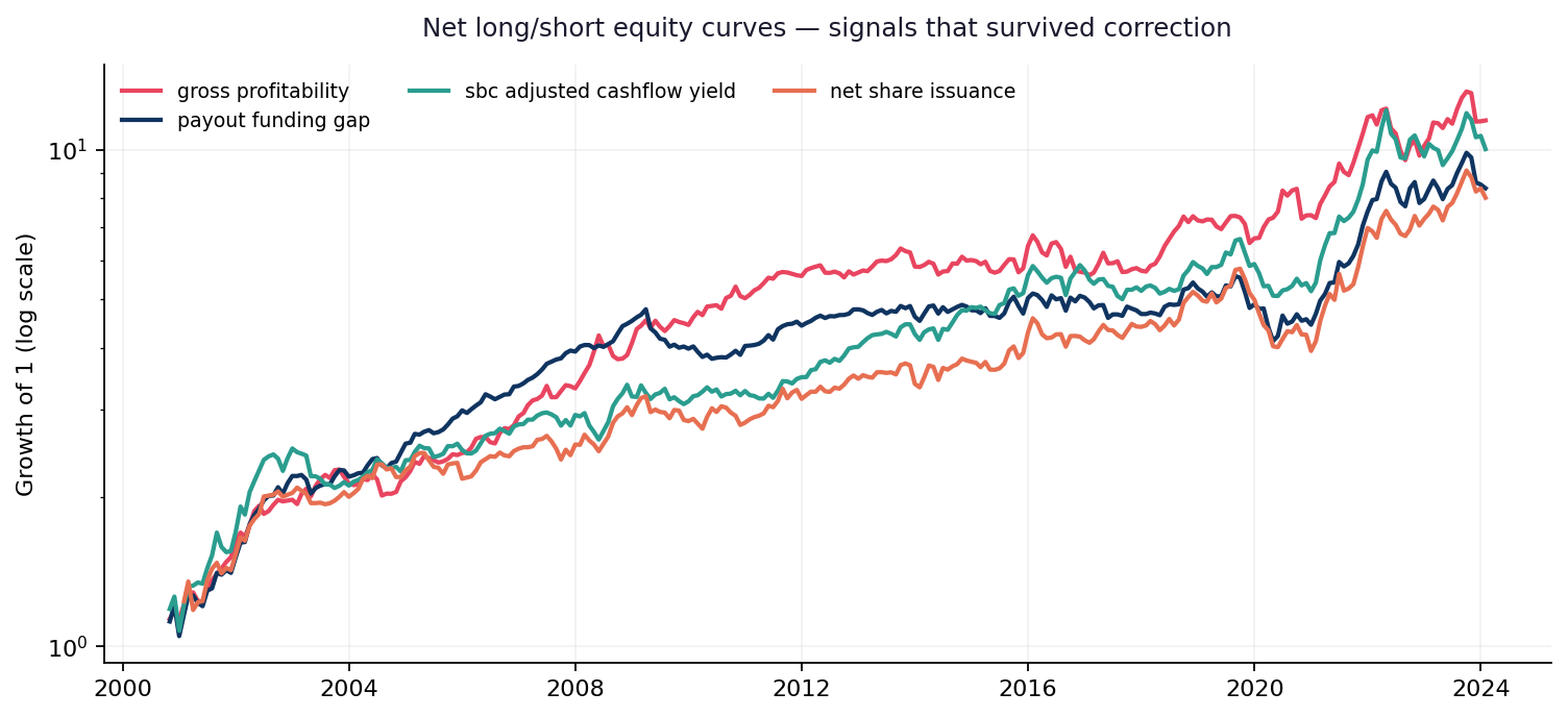
What this run found

• No signal in this run survives correction. With a hurdle Sharpe of 1.01, nothing on the board is currently distinguishable from the best of a random search of the same size — which is itself the honest headline, not a failure of the machinery.

• 10 are factor tilts in disguise. The clearest case is gradual_information_momentum, whose returns are 93% explained by the standard factors with an alpha t-stat of -0.83 — it is not adding anything the four-factor model does not already capture.

• excess_speculative_volatility is the case for looking past raw Sharpe: only 0.29 on its own, but an alpha t-stat of 2.95 once the known factors are stripped out — its raw performance understates it.

• predicted_dividend_month_premium is the inverse warning: it tracks the standard factors closely (95% of variance) yet delivers significantly negative alpha against them (t=-4.06). On this universe and sample you would have been better off holding the plain factor than this construction of it.

All 171 signals, with 95% confidence intervals click to expand

Signal	Verdict	Sharpe	95% CI	Alpha t	Factor R²	Deflated Sharpe	q-value
gross_profitability	Noise	0.92	[0.51, 1.36]	3.22	21%	0.35	0.002
payout_funding_gap	Noise	0.82	[0.40, 1.28]	3.55	42%	0.19	0.011
sbc_adjusted_cashflow_yield	Noise	0.78	[0.38, 1.19]	3.30	55%	0.13	0.015
net_share_issuance	Noise	0.73	[0.36, 1.09]	4.26	59%	0.08	0.015
macro_systematic_variance_share	Noise	0.57	[0.11, 0.98]	1.78	53%	0.03	0.081
cross_sectional_beta_dispersion_timing	Noise	0.51	[0.07, 1.00]	1.10	39%	0.01	0.132
late_quarter_buyback_share_shrinkage	Noise	0.56	[0.20, 0.88]	3.07	70%	0.01	0.061
trade_credit_stretch_quality	Noise	0.51	[0.10, 0.89]	2.60	4%	0.01	0.081
stagflation_supply_shock_timing	Noise	0.52	[0.12, 0.91]	2.59	4%	0.01	0.090
predicted_dividend_month_premium	Loses to factors	0.41	[-0.00, 0.89]	-4.06	95%	0.00	0.204
aggregate_accruals_market_timing	Noise	0.37	[-0.07, 0.78]	1.70	14%	0.00	0.373
asset_growth	Noise	0.43	[0.02, 0.81]	2.27	45%	0.00	0.204
tax_loss_selling_turn_of_year_pressure	Noise	-0.58	[-1.48, 0.18]	-0.73	8%	0.00	0.374
average_systematic_comovement_timing	Noise	0.36	[-0.12, 0.88]	0.25	39%	0.00	0.425
operating_leverage_industrial_cycle	Noise	0.39	[-0.07, 0.81]	1.75	4%	0.00	0.335
retained_vs_contributed_capital_value	Noise	0.38	[0.01, 0.75]	1.76	65%	0.00	0.230
frog_in_the_pan_gradual_momentum	Factor tilt	0.33	[-0.10, 0.76]	1.07	90%	0.00	0.373
lottery_demand_sentiment_interaction	Noise	0.31	[-0.15, 0.79]	1.08	7%	0.00	0.491
earnings_yield	Noise	0.34	[-0.10, 0.80]	-0.00	62%	0.00	0.416
cash_backed_earnings_surprise	Noise	0.28	[-0.13, 0.69]	0.81	57%	0.00	0.441
sentiment_fundamental_pessimism_gap_timing	Noise	0.25	[-0.26, 0.72]	0.45	12%	0.00	0.656
momentum_12_1	Factor tilt	0.27	[-0.16, 0.73]	-0.10	92%	0.00	0.491
excess_speculative_volatility	Noise	0.29	[-0.09, 0.67]	2.95	50%	0.00	0.391
equity_rate_correlation_regime_timing	Noise	0.25	[-0.17, 0.73]	0.18	26%	0.00	0.592
inventory_growth_gap	Noise	0.26	[-0.14, 0.70]	0.22	25%	0.00	0.484
gradual_information_momentum	Factor tilt	0.25	[-0.17, 0.69]	-0.83	93%	0.00	0.543
equity_yield_vs_real_rate_gap_timing	Noise	0.18	[-0.31, 0.70]	-0.75	38%	0.00	0.786
inflation_passthrough_margin_expansion	Noise	0.23	[-0.20, 0.69]	0.75	27%	0.00	0.592
profitless_market_cap_share_timing	Noise	0.18	[-0.42, 0.77]	0.19	18%	0.00	0.811
sticky_cost_downturn_drag	Noise	0.24	[-0.14, 0.62]	-0.15	42%	0.00	0.506
quiet_strength_low_attention_high	Factor tilt	0.22	[-0.20, 0.65]	1.59	85%	0.00	0.592
low_volatility	Noise	0.25	[-0.15, 0.65]	2.39	83%	0.00	0.507
real_yield_shock_timing	Noise	0.13	[-0.27, 0.57]	0.48	2%	0.00	0.811
aggregate_rollover_risk_funding_shock_timing	Noise	0.17	[-0.35, 0.68]	0.45	7%	0.00	0.811
aggregate_equity_issuance_market_timing	Noise	0.20	[-0.34, 0.70]	1.11	7%	0.00	0.786
financial_slack_under_tightening	Noise	0.21	[-0.17, 0.60]	0.38	7%	0.00	0.592
tax_loss_selling_seasonal_reversal	Noise	-0.57	[-1.39, 0.23]	-1.06	19%	0.00	0.433
credit_vol_complacency_divergence_timing	Noise	0.12	[-0.21, 0.51]	-0.47	17%	0.00	0.811
depreciation_conservatism_reserve	Noise	0.20	[-0.27, 0.65]	0.77	4%	0.00	0.745
sentiment_misery_residual_timing	Noise	0.15	[-0.28, 0.55]	0.89	9%	0.00	0.786
seasonal_risk_appetite_credit_timing	Noise	0.20	[-0.19, 0.52]	1.41	4%	0.00	0.649
accruals	Noise	0.18	[-0.25, 0.64]	1.96	21%	0.00	0.745
cash_vs_accounting_value_divergence	Noise	0.19	[-0.25, 0.64]	1.90	26%	0.00	0.746
residual_vix_hedge_premium	Noise	0.18	[-0.25, 0.61]	1.01	15%	0.00	0.720
equity_fear_vs_credit_stress_divergence_timing	Noise	0.09	[-0.25, 0.47]	-1.11	25%	0.00	0.867
macro_beta_rotation_instability	Noise	0.15	[-0.24, 0.54]	1.20	65%	0.00	0.786
effective_tax_rate_earnings_quality	Noise	0.15	[-0.20, 0.51]	0.15	6%	0.00	0.781
sentiment_fundamental_gap_timing	Noise	0.11	[-0.33, 0.54]	0.73	7%	0.00	0.867
market_breadth_high_ratio_timing	Noise	0.12	[-0.24, 0.50]	2.64	24%	0.00	0.811
macro_exposure_drift	Noise	0.13	[-0.26, 0.51]	1.04	66%	0.00	0.811
equity_duration_rate_trend_interaction	Noise	0.13	[-0.37, 0.68]	1.28	7%	0.00	0.858
macro_trend_exposure_alignment	Noise	0.01	[-0.47, 0.48]	0.15	24%	0.00	0.979
unproductive_acquisition_growth	Noise	0.12	[-0.31, 0.58]	-0.27	13%	0.00	0.838
credit_equity_divergence_timing	Noise	0.08	[-0.39, 0.48]	0.21	3%	0.00	0.872
credit_spread_timing	Noise	0.09	[-0.40, 0.52]	0.60	15%	0.00	0.872
market_trend_timing	Noise	0.06	[-0.43, 0.53]	1.17	36%	0.00	0.919
macro_beta_instability	Factor tilt	0.10	[-0.27, 0.45]	1.38	72%	0.00	0.864
credit_beta_defensive	Noise	0.11	[-0.29, 0.44]	0.25	34%	0.00	0.833
oil_beta_trend_interaction	Noise	0.10	[-0.33, 0.50]	-0.49	16%	0.00	0.867
hidden_dilution_sbc_yield	Factor tilt	0.10	[-0.32, 0.50]	-0.82	75%	0.00	0.867
book_to_market	Loses to factors	0.11	[-0.36, 0.58]	-3.14	92%	0.00	0.867
sbc_inflated_operating_cash_flow	Noise	0.10	[-0.37, 0.55]	-1.13	53%	0.00	0.867
macro_momentum_diffusion_timing	Noise	0.06	[-0.46, 0.59]	1.02	29%	0.00	0.930
money_illusion_real_yield_gap_timing	Noise	0.05	[-0.34, 0.49]	-1.86	39%	0.00	0.912
vix_conditioned_reversal_flip	Noise	0.06	[-0.25, 0.39]	-0.70	11%	0.00	0.872
usd_exposure_dollar_trend_interaction	Noise	-0.10	[-0.58, 0.42]	-0.50	25%	0.00	0.867
vix_beta_drift	Noise	0.07	[-0.41, 0.52]	0.02	15%	0.00	0.886
turn_of_year_tax_loss_rebound_intensity	Noise	0.07	[-0.31, 0.46]	0.82	4%	0.00	0.872
macro_trend_beta_alignment	Noise	-0.20	[-0.77, 0.39]	-0.94	40%	0.00	0.809
macro_beta_churn_instability	Factor tilt	0.07	[-0.30, 0.44]	0.88	70%	0.00	0.872
dollar_trend_fx_beta_interaction	Noise	-0.08	[-0.55, 0.39]	-0.58	26%	0.00	0.872
stock_comp_earnings_dilution	Noise	0.08	[-0.39, 0.53]	-1.27	53%	0.00	0.872
macro_exposure_instability	Noise	0.05	[-0.33, 0.41]	0.65	66%	0.00	0.912
net_trade_credit_expansion	Noise	0.04	[-0.31, 0.41]	-0.47	9%	0.00	0.940
stock_comp_burden_yield	Noise	0.04	[-0.36, 0.49]	1.09	24%	0.00	0.944
aggregate_inventory_overhang_timing	Noise	-0.02	[-0.57, 0.48]	1.07	38%	0.00	0.975
dollar_liquidity_cycle_timing	Noise	-0.18	[-0.70, 0.47]	0.32	17%	0.00	0.811
unemployment_news_regime_asymmetry_timing	Noise	-0.02	[-0.58, 0.55]	0.55	13%	0.00	0.979
macro_beta_churn	Noise	0.03	[-0.34, 0.39]	0.73	70%	0.00	0.950
macro_beta_instability_ambiguity	Noise	0.03	[-0.34, 0.39]	0.73	70%	0.00	0.950
cross_sectional_return_dispersion_timing	Noise	-0.05	[-0.62, 0.45]	0.49	28%	0.00	0.944
macro_pessimism_contrarian_market_timing	Noise	0.00	[-0.54, 0.51]	-0.16	5%	0.00	0.986
aggregate_inventory_sales_cycle_timing	Noise	-0.02	[-0.40, 0.37]	0.04	6%	0.00	0.975
rate_duration_mispricing	Noise	0.03	[-0.36, 0.50]	1.05	29%	0.00	0.963
funding_conditioned_beta_tilt	Noise	0.03	[-0.35, 0.38]	-0.47	7%	0.00	0.950
book_tax_gap_earnings_quality	Noise	0.03	[-0.38, 0.42]	-0.97	13%	0.00	0.966
variance_risk_premium_timing	Noise	-0.01	[-0.46, 0.45]	-1.67	31%	0.00	0.986
aggregate_earnings_growth_breadth_timing	Noise	-0.05	[-0.52, 0.40]	-0.51	21%	0.00	0.944
unemployment_trough_breakout_timing	Noise	-0.02	[-0.57, 0.56]	0.22	10%	0.00	0.979
sentiment_fundamental_divergence_timing	Noise	-0.10	[-0.67, 0.43]	-0.12	17%	0.00	0.872
macro_risk_on_breadth_contrarian_timing	Noise	-0.02	[-0.50, 0.43]	-1.08	30%	0.00	0.979
rollover_risk_credit_cycle_interaction	Noise	0.01	[-0.39, 0.45]	1.40	12%	0.00	0.979
aggregate_illiquidity_shock_timing	Noise	-0.04	[-0.50, 0.36]	-1.47	29%	0.00	0.950
turn_of_year_tax_loss_pressure	Noise	-0.96	[-1.85, -0.15]	-1.16	22%	0.00	0.128
sahm_labor_deterioration_timing	Noise	-0.02	[-0.61, 0.53]	0.20	11%	0.00	0.979
hidden_rate_duration_mismatch	Noise	-0.01	[-0.47, 0.51]	1.13	12%	0.00	0.986
long_term_reversal_sentiment_conditioned	Noise	-0.10	[-0.65, 0.40]	-0.87	40%	0.00	0.867
sentiment_gap_contrarian_timing	Noise	-0.12	[-0.74, 0.50]	-0.69	9%	0.00	0.867
aggregate_turnover_sentiment_timing	Noise	-0.10	[-0.52, 0.37]	-1.43	20%	0.00	0.867
household_sentiment_fundamental_divergence_timing	Noise	-0.17	[-0.63, 0.30]	-1.11	11%	0.00	0.802
sentiment_fundamental_disagreement_timing	Noise	-0.23	[-0.71, 0.20]	-0.84	9%	0.00	0.592
sentiment_capitulation_recovery_timing	Noise	-0.09	[-0.58, 0.44]	-0.58	14%	0.00	0.872
labor_cycle_turning_point_timing	Noise	-0.21	[-0.86, 0.36]	-0.02	29%	0.00	0.803
hidden_equity_dilution_cost	Noise	-0.08	[-0.52, 0.28]	-1.31	59%	0.00	0.867
attention_shock_amplified_reversal	Noise	-0.09	[-0.46, 0.25]	-2.14	22%	0.00	0.867
halloween_volatility_scaled_timing	Noise	-0.11	[-0.47, 0.27]	0.30	5%	0.00	0.838
hidden_refinancing_rate_exposure	Noise	-0.07	[-0.41, 0.27]	-1.71	16%	0.00	0.867
cross_asset_news_diffusion_momentum	Noise	-0.08	[-0.48, 0.32]	0.38	8%	0.00	0.872
sentiment_hard_data_divergence_timing	Noise	-0.21	[-0.72, 0.27]	-0.55	21%	0.00	0.745
fundamental_momentum_price_gap	Factor tilt	-0.10	[-0.43, 0.26]	0.55	72%	0.00	0.838
net_cash_yield_rate_change_interaction	Noise	-0.09	[-0.48, 0.32]	-1.04	12%	0.00	0.867
credit_sensitivity_amplified_balance_sheet_safety	Noise	-0.10	[-0.55, 0.34]	2.54	60%	0.00	0.867
macro_trend_beta_spillover	Noise	-0.17	[-0.60, 0.28]	-0.99	35%	0.00	0.786
macro_trend_attributed_return_reversal	Noise	-0.13	[-0.47, 0.25]	0.13	39%	0.00	0.803
transitory_nonoperating_income_intensity	Noise	-0.14	[-0.59, 0.30]	-0.08	39%	0.00	0.822
consumer_sentiment_credit_divergence_timing	Noise	-0.24	[-0.67, 0.19]	-1.41	7%	0.00	0.636
real_policy_stance_timing	Noise	-0.16	[-0.55, 0.33]	-2.07	21%	0.00	0.802
seasonal_same_month_return_persistence	Noise	-0.28	[-0.76, 0.11]	-1.44	53%	0.00	0.441
macro_beta_dispersion_crowding_rotation	Noise	-0.17	[-0.62, 0.23]	-1.97	24%	0.00	0.774
abnormal_reporting_lag	Noise	-0.16	[-0.60, 0.29]	0.17	21%	0.00	0.802
rate_beta_duration_mismatch	Noise	-0.20	[-0.74, 0.25]	-2.15	13%	0.00	0.664
valuation_dispersion_market_timing	Noise	-0.31	[-0.83, 0.17]	-0.22	32%	0.00	0.491
conditional_size_credit_cycle	Noise	-0.25	[-0.71, 0.23]	-1.02	12%	0.00	0.592
operating_leverage_business_cycle	Noise	-0.19	[-0.69, 0.28]	-0.56	3%	0.00	0.786
pure_calendar_month_seasonality_spread	Noise	-0.29	[-0.70, 0.12]	-1.61	5%	0.00	0.441
attention_shock_at_the_highs	Loses to factors	-0.29	[-0.69, 0.09]	-2.96	84%	0.00	0.373
taylor_rule_policy_accommodation_timing	Noise	-0.35	[-0.72, 0.07]	-2.65	16%	0.00	0.372
working_capital_release_under_tightening	Noise	-0.29	[-0.68, 0.10]	-0.56	7%	0.00	0.402
seasonal_same_month_residual_return	Noise	-0.38	[-0.81, 0.01]	-1.92	4%	0.00	0.254
attention_shock_return_reversal	Noise	-0.42	[-0.78, -0.10]	-3.92	31%	0.00	0.053
turnover_shock_price_run_reversal	Noise	-0.42	[-0.78, -0.10]	-3.92	31%	0.00	0.053
earnings_smoothing_detection	Noise	-0.35	[-0.81, 0.15]	-2.36	34%	0.00	0.425
same_quarter_earnings_seasonality	Noise	-0.29	[-0.72, 0.16]	-0.68	23%	0.00	0.441
sbc_inflated_cash_earnings	Loses to factors	-0.31	[-0.78, 0.12]	-3.55	61%	0.00	0.391
credit_beta_leverage_mismatch	Factor tilt	-0.28	[-0.63, 0.10]	0.22	73%	0.00	0.439
same_month_return_seasonality_spread	Noise	-0.45	[-0.95, 0.02]	-1.72	13%	0.00	0.219
oil_shock_demand_supply_timing	Noise	-0.30	[-0.68, 0.12]	-1.32	13%	0.00	0.433
unpriced_leverage_credit_insensitivity	Factor tilt	-0.32	[-0.66, 0.05]	-0.14	73%	0.00	0.369
oil_demand_vs_supply_shock_timing	Noise	-0.40	[-0.83, 0.01]	-1.42	3%	0.00	0.280
earnings_smoothing_opacity	Noise	-0.42	[-0.85, 0.01]	-2.74	41%	0.00	0.261
earnings_smoothness_vs_cashflow	Noise	-0.42	[-0.86, 0.00]	-2.78	41%	0.00	0.258
earnings_smoothing_vs_cashflow_volatility	Noise	-0.41	[-0.84, 0.01]	-2.58	42%	0.00	0.249
same_month_return_seasonality	Noise	-0.65	[-1.19, -0.18]	-2.59	10%	0.00	0.046
annual_return_seasonality_spread	Noise	-0.66	[-1.20, -0.19]	-2.60	10%	0.00	0.046
external_finance_dependence_credit_shock	Noise	-0.46	[-0.90, -0.01]	-1.96	1%	0.00	0.165
annual_return_seasonality_purged	Noise	-0.62	[-1.11, -0.18]	-2.03	4%	0.00	0.061
same_month_seasonality_ex_adjacent	Noise	-0.62	[-1.11, -0.18]	-2.03	4%	0.00	0.061
size_premium_credit_conditions_switch	Noise	-0.44	[-0.85, -0.03]	-2.13	12%	0.00	0.199
same_month_seasonality_excess	Noise	-0.65	[-1.13, -0.24]	-2.45	4%	0.00	0.039
relative_month_of_year_seasonality	Noise	-0.65	[-1.15, -0.23]	-2.27	4%	0.00	0.040
same_month_seasonality_residual	Noise	-0.65	[-1.15, -0.23]	-2.27	4%	0.00	0.040
annual_return_seasonality	Noise	-0.70	[-1.26, -0.24]	-2.53	7%	0.00	0.039
zero_earnings_threshold_management	Noise	-0.56	[-1.00, -0.16]	-1.06	46%	0.00	0.048
same_month_seasonal_persistence	Noise	-0.69	[-1.12, -0.30]	-2.68	3%	0.00	0.015
pre_earnings_filing_clock_premium	Noise	-0.47	[-0.85, -0.10]	-2.51	2%	0.00	0.073
hidden_credit_risk_mismatch	Noise	-0.48	[-0.81, -0.15]	-1.29	46%	0.00	0.079
same_month_minus_offseason_seasonality	Noise	-0.73	[-1.20, -0.30]	-3.02	5%	0.00	0.021
same_calendar_month_return_seasonality	Noise	-0.71	[-1.27, -0.22]	-2.96	3%	0.00	0.040
same_calendar_month_seasonality	Noise	-0.71	[-1.27, -0.22]	-2.96	3%	0.00	0.040
leverage_credit_beta_complacency	Noise	-0.51	[-0.86, -0.19]	-1.40	49%	0.00	0.061
stock_comp_dilution_earnings_overstatement	Noise	-0.58	[-1.08, -0.06]	-3.40	43%	0.00	0.090
residual_same_month_seasonality	Noise	-0.80	[-1.32, -0.32]	-3.36	5%	0.00	0.015
same_month_annual_seasonality	Noise	-0.75	[-1.33, -0.25]	-3.15	2%	0.00	0.035
same_month_seasonal_return_persistence	Noise	-0.75	[-1.33, -0.25]	-3.15	2%	0.00	0.035
expected_earnings_announcement_month	Noise	-0.57	[-0.95, -0.20]	-2.46	3%	0.00	0.046
tax_loss_overhang_seasonal	Noise	-0.50	[-0.90, -0.06]	-1.82	6%	0.00	0.131
tax_loss_selling_turn_of_year_reversal	Noise	-0.47	[-0.78, -0.11]	-2.26	3%	0.00	0.081
attention_spike_return_reversal	Noise	-0.75	[-1.28, -0.33]	-5.32	10%	0.00	0.004
tax_loss_overhang_turn_of_year	Noise	-0.45	[-0.73, -0.12]	-2.28	2%	0.00	0.104
macro_loading_instability	Noise	-0.70	[-1.08, -0.31]	-3.42	10%	0.00	0.015
filing_staleness_information_neglect	Noise	-1.05	[-1.47, -0.67]	-4.39	1%	0.00	0.000

Best signal vs the market

The top of the board is gross_profitability. Here it is against a large-cap benchmark — the 500 biggest eligible names each month, cap-weighted, rebalanced monthly, run through the identical point-in-time and delisting machinery.

Cumulative growth and drawdown of the best signal against the cap-weighted large-cap benchmark. Log scale on the upper panel.

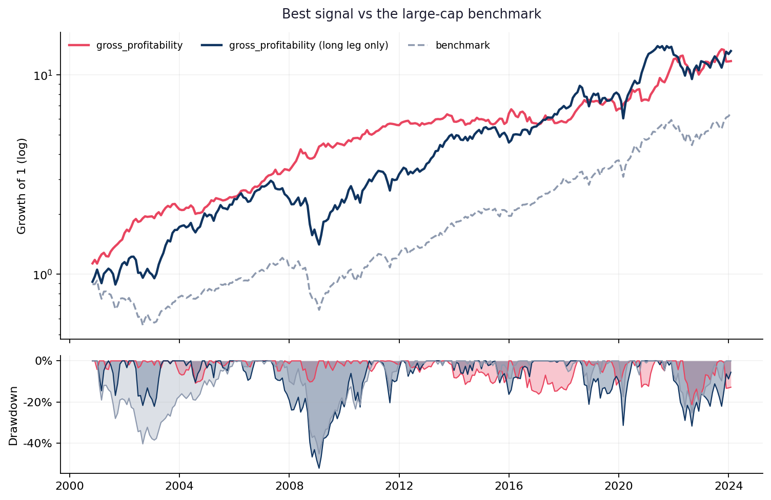
Metric	gross_profitability	Benchmark
Annualized return	11.1%	8.3%
Annualized volatility	12.3%	15.5%
Sharpe ratio	0.92	0.60
Max drawdown	-21.3%	-45.2%
Hit rate (months up)	62.9%	65.4%

These are not the same kind of return. The signal is a market-neutral long/short book: it holds the top decile and shorts the bottom, so it carries almost no market exposure and its return does not depend on the market going up. The benchmark is long-only and fully exposed. Comparing their raw returns rewards whichever one happened to suit the sample — the relationship between them is the informative part:

Correlation to the benchmark is -0.11 and beta is -0.09. A beta near zero is the point of a long/short construction, not a shortfall: it means the return is not repackaged market exposure. Up-capture is 19% and down-capture -39% — how much of the market’s average up-month and down-month the strategy tracked. Low or negative down-capture is the property a diversifying book is actually bought for.

Measured over 280 overlapping months. A market-neutral book with a lower headline return than a bull-market index can still be the more valuable asset in a portfolio, because it supplies a return stream the index cannot.

The factors and the statistics, in depth

The four factors — what they are and how they are built here click to expand

A new signal is only interesting if it earns something the known premia do not already pay for. These four are the standard yardstick. All are built from the same panel the signals are scored on — equal-weighted top-third minus bottom-third spreads on the same eligible universe — so attribution is like-for-like rather than against an external dataset with different conventions.

MKT — Market

The excess return of holding equities at all. Every long-only strategy earns most of its return here, so it is the first thing to strip out.Built here as: Equal-weighted return of the whole eligible universe each month.

SMB — Size (small minus big)

Small-cap stocks have historically earned more than large caps — compensation for illiquidity and distress risk, and partly a reflection of how hard small names are to trade at size.Built here as: Long the smallest third by market cap, short the largest third.

HML — Value (high minus low)

Cheap stocks relative to book value have outearned expensive ones. The debate over whether this is risk compensation or a behavioural mispricing is unsettled; either way it is a known, harvestable premium, so a new signal should not be paid twice for it.Built here as: Long the cheapest third by price-to-book, short the most expensive third.

UMD — Momentum (up minus down)

Past winners keep winning over horizons of roughly three to twelve months, usually attributed to under-reaction to news and to slow diffusion of information.Built here as: Long the top third by 12-1 month return, short the bottom third.

The statistics — what each one answers, and the failure it guards against click to expand

Each statistic exists because a simpler one can be fooled in a specific way. Read top to bottom and the argument builds: a Sharpe is not enough, so bound it; a bound is not enough on skewed returns, so reshape it; and none of it means anything until you price in how many strategies were tried to find this one.

Sharpe ratio

Return per unit of volatility, annualized. The default headline — and the single most misleading number on any farmed leaderboard, because it says nothing about how many strategies were tried before this one was picked.Sharpe = mean(r) / sd(r) × √12

Guards against: Says nothing about selection. Rewards fat left tails.

95% confidence interval

A circular block bootstrap resamples contiguous blocks of months — preserving short-run autocorrelation an i.i.d. bootstrap would destroy — and re-computes the Sharpe a few thousand times. The interval is the middle 95% of that distribution. If it straddles zero, the point estimate is not doing the work you think it is.block length ≈ T^(1/3), 2,000 resamples

Guards against: A single Sharpe with no interval invites false confidence.

Newey-West t-statistic

The t-stat of the mean return, with standard errors corrected for autocorrelation and heteroskedasticity. Monthly strategy returns are rarely independent, and ignoring that inflates significance.t = mean(r) / SE_NW(r), lags = ⌊4(T/100)^(2/9)⌋

Guards against: Plain OLS errors overstate significance on persistent series.

Factor R²

The share of the strategy’s month-to-month variance explained by regressing it on market, size, value and momentum. High R² means you have largely rebuilt a portfolio of things that already have names.R² from r_t = α + β₁MKT + β₂SMB + β₃HML + β₄UMD + ε_t

Guards against: A high Sharpe can be entirely factor exposure.

Alpha t-statistic

The intercept of that same regression — the return the four factors cannot explain — divided by its Newey-West standard error. This is the closest thing here to a test of whether a signal is genuinely new. Note the sign: a large negative alpha t means the construction loses to the factor it tracks.α from the regression above; t = α / SE_NW(α)

Guards against: Sharpe alone cannot tell a discovery from a repackaged tilt.

Probabilistic Sharpe (PSR)

The probability the true Sharpe exceeds zero, adjusted for skew and kurtosis. Strategies that make small gains most months and lose badly occasionally — the classic short-leg blow-up shape — get marked down relative to their raw Sharpe.PSR = Φ( (SR − SR*)·√(T−1) / √(1 − γ₃SR + (γ₄−1)SR²/4) )

Guards against: Raw Sharpe assumes normality that returns rarely have.

Search hurdle

The Sharpe you would expect from the best of N random strategies, given how dispersed the Sharpes in this library actually are. It is the bar luck alone clears. Anything under it is not evidence of anything.E[max SR] ≈ √V · [ (1−γ)Φ⁻¹(1 − 1/N) + γΦ⁻¹(1 − 1/(Ne)) ]

Guards against: Testing many strategies guarantees a good-looking winner.

Deflated Sharpe (DSR)

The PSR measured against that hurdle instead of against zero: the probability the signal is real given the size of the search that found it. This is what the board is sorted by. N counts every farming attempt in the ledger — including the ideas that died at the data or compile stage — because counting only survivors would understate the search and flatter every number.DSR = PSR evaluated at SR* = E[max SR]

Guards against: The headline result of a bulk search is biased upward by construction.

Benjamini-Hochberg q-value

Ranks every p-value in the library and controls the expected proportion of false discoveries among those called significant. Far less brutal than Bonferroni when signals are correlated — which factor strategies always are — while still bounding the damage.q_(i) = min over j ≥ i of p_(j) · m / j

Guards against: Per-signal p-values ignore that the library is a search.

How to read a row in one pass. Start at the deflated Sharpe: if it is low, nothing else on the row rescues the signal. If it is high, check the alpha t-stat to see whether the return is genuinely new or a factor tilt wearing a different name. Then check the confidence interval: if it straddles zero, the sample is too short to lean on regardless of what the point estimates say.

Run history

Run	Signals	Survivors	Hurdle	Best Sharpe
2026-10-02	171	0	1.01	0.92
2026-09-15	170	0	1.00	0.92
2026-09-02	121	0	0.95	0.92
2026-09-01	113	0	0.95	0.92
2026-08-31	102	0	0.95	0.92
2026-08-30	96	0	0.94	0.92
2026-08-29	88	0	0.92	0.92
2026-08-27	77	0	0.89	0.92
2026-08-26	69	0	0.89	0.92
2026-08-25	58	0	0.83	0.92
2026-08-24	48	0	0.75	0.92
2026-08-23	39	0	0.66	0.92

Where this goes next

The pipeline works; the constraint now is the hypothesis space, not the machinery. Ranked roughly by expected value per unit of effort:

Widen the data surface

Every signal is bounded by what the panel contains. The highest-leverage additions are short interest and borrow cost (crowding and limits to arbitrage), institutional 13F holdings (ownership churn), analyst revisions and dispersion (expectation dynamics), and options-implied volatility surfaces (skew as a crash-risk premium). Each new provider under data/features/ multiplies the hypothesis space rather than adding to it.

high impact · medium effort

Walk-forward, not full-sample

The harness currently scores each signal over the whole history. A purged, embargoed walk-forward protocol — fit and select on an expanding window, evaluate only on the untouched next block — would turn every number on this page into an out-of-sample one, and would catch signals that only work in the regime they were invented from.

high impact · medium effort

Let the agents read their own failures

The idea agent sees which themes are thin, but not why past ideas died. Feeding back the specific failure — the validator’s complaint, the coverage gate, the factor attribution that revealed a tilt — should raise the hit rate per unit of spend, and it costs nothing but prompt tokens.

high impact · low effort

Search combinations, not just singles

Most published anomalies are weak alone and strong combined. A composite layer — rank-average within a theme, or a shrunk regression on standardized signals — would test whether the farmed library is greater than its parts. The novelty machinery already stores the return streams needed for it.

medium impact · low effort

Model capacity honestly

Costs are a flat per-unit-traded charge. Real capacity binds through market impact that scales with size and inversely with liquidity. A square-root impact model plus an explicit AUM assumption would tell us which of these signals survive at size rather than only on paper.

medium impact · medium effort

Turn the delisting assumption into a measurement

Delisted names currently book a configurable return, defaulted to a liquidation at the last observed price. Sharadar’s corporate-actions table carries the actual delisting events; using them would replace an assumption with data, and would matter most for exactly the distressed, cheap names that value signals load on.

medium impact · low effort

Regime-condition the evaluation

A signal that works only in high-dispersion or high-rate regimes is still useful — if you know which regime you are in. Conditioning the report on macro states already in the panel would separate genuinely broken signals from ones that are simply out of season.

medium impact · medium effort

Raise the bar as the library grows

The deflation hurdle scales with the number of trials, so the more this pipeline runs, the harder it becomes to claim a discovery — correctly. The counter-move is not a lower bar but a better prior: pre-register the economic mechanism before the backtest, and treat signals whose mechanism was stated in advance as a separate, smaller family of tests.

structural · ongoing

The honest summary is that a language model is a good generator of plausible hypotheses and a poor judge of which ones are real. That division of labour is the whole design: let the model propose freely, and make the harness — not the model — decide what counts.

The signal library

All 171 signals — what each one measures, and the code that computes it click to expand

One entry per signal currently in the library: the reference anomalies from the literature and every agent-written signal that compiled and passed validation. The calculation shown is the compute method itself, read straight out of the module at publish time — the page cannot drift away from the code it documents. Each returns a raw score; the harness multiplies it by the expected sign, so after orientation a high score always means “go long”.

Cross-sectional signals (122)

Scored for every stock every month. The strategy is long the top third of the oriented score and short the bottom third, rebalanced monthly.

credit_sensitivity_amplified_balance_sheet_safetycomboInteraction of credit-beta sensitivity with fundamental balance-sheet safety: among stocks whose returns load…

Interaction of credit-beta sensitivity with fundamental balance-sheet safety: among stocks whose returns load heavily on credit-market moves, those with low leverage, high EBIT coverage, high liquidity and cash reserves are over-discounted and expected to outperform.

Category comboDirection Long the high scoresData price, fundamental, macro

def compute(self, panel) -> pd.Series:
    debt = panel['debt']
    assets = panel['assets']
    ebit = panel['ebit']
    currentratio = panel['currentratio']
    cashneq = panel['cashneq']
    liabilities = panel['liabilities']
    beta_credit = panel['beta_credit_252']
    # base validity mask: require all raw inputs present
    base_valid = (
        debt.notna() & assets.notna() & ebit.notna() &
        currentratio.notna() & cashneq.notna() &
        liabilities.notna() & beta_credit.notna()
    )
    assets_pos = assets > 0
    debt_pos = debt > 0
    lev = pd.Series(np.nan, index=panel.index)
    lev_mask = base_valid & assets_pos
    lev.loc[lev_mask] = debt.loc[lev_mask] / assets.loc[lev_mask]
    denom = pd.Series(np.nan, index=panel.index)
    cov_mask = base_valid & debt_pos
    denom.loc[cov_mask] = debt.loc[cov_mask]
    # fallback to eps-like max(debt, eps) per formula, but eps not mapped -> use debt only
    cov = pd.Series(np.nan, index=panel.index)
    cov.loc[cov_mask] = ebit.loc[cov_mask] / denom.loc[cov_mask]
    cov = cov.clip(-5, 5)
    liq = currentratio.clip(upper=5)
    liq = liq.where(base_valid)
    cashr = pd.Series(np.nan, index=panel.index)
    cashr.loc[lev_mask] = cashneq.loc[lev_mask] / assets.loc[lev_mask]
    df = pd.DataFrame({
        'lev': lev,
        'cov': cov,
        'liq': liq,
        'cashr': cashr,
        'beta_credit': beta_credit.where(base_valid),
    }, index=panel.index)
    def per_date(g: pd.DataFrame) -> pd.Series:
        valid_rows = g[['lev', 'cov', 'liq', 'cashr', 'beta_credit']].notna().all(axis=1)
        g_valid = g.loc[valid_rows]
        out = pd.Series(np.nan, index=g.index)
        if g_valid.empty:
            return out
        z_lev = self._zscore(g_valid['lev'])
        z_cov = self._zscore(g_valid['cov'])
        z_liq = self._zscore(g_valid['liq'])
        z_cashr = self._zscore(g_valid['cashr'])
        safety = -z_lev + 0.5 * z_cov + 0.5 * z_liq + 0.5 * z_cashr
        abs_beta = g_valid['beta_credit'].abs()
        w = abs_beta.rank(pct=True)
        sig = safety * (0.25 + w)
        out.loc[g_valid.index] = sig
        return out
    raw_signal = df.groupby(level='date', group_keys=False).apply(per_date)
    # macro_baa_spread past-only z-score scaling
    baa = panel['macro_baa_spread']
    baa_by_date = baa.groupby(level='date').first()
    baa_by_date = baa_by_date.sort_index()
    mean_rolling = baa_by_date.expanding(min_periods=2).mean().shift(1)
    std_rolling = baa_by_date.expanding(min_periods=2).std().shift(1)
    z_baa = (baa_by_date - mean_rolling) / std_rolling
    z_baa = z_baa.replace([np.inf, -np.inf], np.nan)
    z_baa_clipped = z_baa.clip(-1, 1)
    multiplier = 1 + 0.5 * z_baa_clipped
    multiplier = multiplier.fillna(1.0)
    multiplier_full = panel.index.get_level_values('date').map(multiplier)
    multiplier_full = pd.Series(multiplier_full, index=panel.index)
    result = raw_signal * multiplier_full
    result.name = self.name
    return result

funding_conditioned_beta_tiltcomboFlips the sign of the beta tilt with the funding-liquidity cycle, measured by the joint 12-month change in…

Flips the sign of the beta tilt with the funding-liquidity cycle, measured by the joint 12-month change in fed funds rate and Baa credit spread. During funding easing episodes, high-beta names are favored; during tightening, low-beta names are favored.

Category comboDirection Long the high scoresData price, macro

def compute(self, panel) -> pd.Series:
    beta = panel['beta_252']
    fedfunds_chg = panel['macro_fedfunds_chg12m']
    baa_chg = panel['macro_baa_spread_chg12m']
    nobs = panel['nobs']
    tighten = fedfunds_chg + baa_chg
    ease = -tighten
    score = beta * np.tanh(ease)
    invalid = beta.isna() | fedfunds_chg.isna() | baa_chg.isna() | (nobs < 200)
    score = score.where(~invalid, np.nan)
    return score.reindex(panel.index)

net_cash_yield_rate_change_interactioncomboInteraction between net-cash-to-marketcap ratio and the signed 12-month change in the 2-year Treasury yield

Interaction between net-cash-to-marketcap ratio and the signed 12-month change in the 2-year Treasury yield. Cash-rich firms benefit from rising short rates via interest income while net-debt firms benefit from falling rates via cheaper refinancing; this macro-conditioned quality/leverage signal flips sign with the direction of the short-rate cycle.

Category comboDirection Long the high scoresData fundamental, price, macro

def compute(self, panel) -> pd.Series:
    cashneq = panel['cashneq']
    debt = panel['debt']
    marketcap = panel['marketcap']
    cond = panel['macro_dgs2_chg12m']
    valid = cashneq.notna() & debt.notna() & marketcap.notna() & (marketcap > 0) & cond.notna()
    net_cash_yield = (cashneq - debt) / marketcap
    net_cash_yield = net_cash_yield.where(valid)
    def winsorize(s):
        if s.notna().sum() == 0:
            return s
        lo = s.quantile(0.01)
        hi = s.quantile(0.99)
        return s.clip(lower=lo, upper=hi)
    net_cash_yield_w = net_cash_yield.groupby(level='date').transform(winsorize)
    signal = net_cash_yield_w * cond
    signal = signal.where(valid)
    return signal.reindex(panel.index)

operating_leverage_business_cyclecomboOperating leverage (opex/assets) conditioned on the trailing 12m change in industrial production and…

Operating leverage (opex/assets) conditioned on the trailing 12m change in industrial production and recession state: high fixed-cost intensity firms are expected to outperform when industrial activity is improving (and underperform when it is deteriorating), capturing a macro-state-dependent risk premium orthogonal to static value/quality factors.

Category comboDirection Long the high scoresData fundamental, macro

def compute(self, panel) -> pd.Series:
    opex = panel['opex']
    assets = panel['assets']
    revenue = panel['revenue']
    valid = (assets > 0) & (revenue > 0)
    ol = (opex / assets).where(valid)
    ol_clipped = ol.clip(lower=0, upper=2)
    def zscore(s):
        mu = s.mean()
        sd = s.std()
        if sd is None or sd == 0 or pd.isna(sd):
            return pd.Series(np.nan, index=s.index)
        return (s - mu) / sd
    ol_z = ol_clipped.groupby(level='date').transform(zscore)
    indpro_chg = panel['macro_indpro_chg12m']
    usrec = panel['macro_usrec']
    cyc = np.tanh(indpro_chg / 2.0) * (1 - 0.5 * usrec)
    cyc = cyc.where(indpro_chg.notna() & usrec.notna())
    raw = ol_z * cyc
    return raw.reindex(panel.index)

rollover_risk_credit_cycle_interactioncomboInteraction between near-term rollover risk (net current debt / assets) and the 12-month change in the…

Interaction between near-term rollover risk (net current debt / assets) and the 12-month change in the Baa-Treasury credit spread. Firms with high net short-term debt suffer when credit spreads widen and benefit when spreads tighten, so the score sign-flips with the credit cycle.

Category comboDirection Long the high scoresData fundamental, macro, price

def compute(self, panel) -> pd.Series:
    debtc = panel['debtc']
    cashneq = panel['cashneq']
    assets = panel['assets']
    tighten = panel['macro_baa_spread_chg12m']
    valid = debtc.notna() & cashneq.notna() & assets.notna() & tighten.notna() & (assets > 0)
    rollover = (debtc - cashneq) / assets.where(assets > 0)
    rollover = rollover.clip(-1, 1)
    score = -rollover * tighten
    score = score.where(valid, np.nan)
    return score.reindex(panel.index)

asset_growthinvestmentCooper-Gulen-Schill asset growth (YoY); low-growth firms outperform

Cooper-Gulen-Schill asset growth (YoY); low-growth firms outperform.

Category investmentDirection Long the low scores

def compute(self, panel: pd.DataFrame) -> pd.Series:
    assets = panel["assets"].where(panel["assets"] > 0)
    return _yoy(assets)

external_finance_dependence_credit_shockinvestmentRajan-Zingales style external finance dependence (capex exceeding internal operating cash flow) combined with…

Rajan-Zingales style external finance dependence (capex exceeding internal operating cash flow) combined with short-term debt load, interacted with the 12-month change in the Baa credit spread. Firms with high financing need are hurt when credit spreads widen and helped when spreads tighten; the harness orients the score so that expected sign is positive.

Category investmentDirection Long the high scoresData fundamental, macro

def compute(self, panel) -> pd.Series:
    assets = panel['assets']
    capex = panel['capex']
    ncfo = panel['ncfo']
    debtc = panel['debtc']
    macro_chg = panel['macro_baa_spread_chg12m']
    valid_assets = assets > 0
    dep = pd.Series(np.nan, index=panel.index)
    stdebt = pd.Series(np.nan, index=panel.index)
    dep_valid = valid_assets & capex.notna() & ncfo.notna() & assets.notna()
    dep.loc[dep_valid] = (capex.loc[dep_valid].abs() - ncfo.loc[dep_valid]) / assets.loc[dep_valid]
    stdebt_valid = valid_assets & debtc.notna() & assets.notna()
    stdebt.loc[stdebt_valid] = debtc.loc[stdebt_valid] / assets.loc[stdebt_valid]
    base_missing = (
        (~valid_assets)
        | capex.isna()
        | ncfo.isna()
        | assets.isna()
        | debtc.isna()
        | macro_chg.isna()
    )
    dep = dep.where(~base_missing)
    stdebt = stdebt.where(~base_missing)
    def cross_section_z(group: pd.Series) -> pd.Series:
        n_valid = group.notna().sum()
        if n_valid < 20:
            return pd.Series(np.nan, index=group.index)
        return _zscore(group)
    dep_z = dep.groupby(level='date').apply(cross_section_z)
    dep_z.index = dep_z.index.droplevel(0) if isinstance(dep_z.index, pd.MultiIndex) and dep_z.index.nlevels > panel.index.nlevels else dep_z.index
    stdebt_z = stdebt.groupby(level='date').apply(cross_section_z)
    stdebt_z.index = stdebt_z.index.droplevel(0) if isinstance(stdebt_z.index, pd.MultiIndex) and stdebt_z.index.nlevels > panel.index.nlevels else stdebt_z.index
    need = dep_z + stdebt_z
    tight = np.tanh(macro_chg / 0.5)
    raw_signal = -need * tight
    raw_signal = raw_signal.where(~base_missing)
    return raw_signal.reindex(panel.index)

inventory_growth_gapinvestmentGap between inventory growth and sales growth over trailing 12 months

Gap between inventory growth and sales growth over trailing 12 months. High inventory growth relative to sales growth signals over-optimistic demand forecasts, future write-downs, and margin pressure, predicting negative future abnormal returns.

Category investmentDirection Long the low scoresData fundamental

def compute(self, panel) -> pd.Series:
    inventory = panel['inventory']
    revenue = panel['revenue']
    assets = panel['assets']
    inv_l12 = inventory.groupby(level='ticker').shift(12)
    rev_l12 = revenue.groupby(level='ticker').shift(12)
    inv_g = pd.Series(np.nan, index=panel.index)
    valid_inv = inv_l12 > 0
    inv_g[valid_inv] = inventory[valid_inv] / inv_l12[valid_inv] - 1.0
    sales_g = pd.Series(np.nan, index=panel.index)
    valid_rev = rev_l12 > 0
    sales_g[valid_rev] = revenue[valid_rev] / rev_l12[valid_rev] - 1.0
    inv_g_clipped = inv_g.clip(-1, 3)
    sales_g_clipped = sales_g.clip(-1, 3)
    raw = inv_g_clipped - sales_g_clipped
    valid_mask = (
        (assets > 0)
        & (inventory > 0)
        & (inv_l12 > 0)
        & (revenue > 0)
        & (rev_l12 > 0)
    )
    raw = raw.where(valid_mask, np.nan)
    return raw

late_quarter_buyback_share_shrinkageinvestmentSignal detects late-quarter share buybacks by comparing weighted-average shares to point-in-time basic shares…

Signal detects late-quarter share buybacks by comparing weighted-average shares to point-in-time basic shares outstanding: sharesbas materially below shareswa implies repurchases concentrated late in the quarter, not yet reflected in annual issuance measures. The signal is confirmed with actual cash outflow for equity (negative ncfcommon relative to market cap) to filter mechanical share-count artifacts.

Category investmentDirection Long the high scoresData fundamental, price

def compute(self, panel) -> pd.Series:
    shareswa = panel['shareswa']
    sharesbas = panel['sharesbas']
    ncfcommon = panel['ncfcommon']
    marketcap = panel['marketcap']
    valid_shares = (shareswa > 0) & (sharesbas > 0)
    shrink = (shareswa - sharesbas) / shareswa.where(shareswa > 0)
    shrink = shrink.where(valid_shares)
    cash_conf = (-ncfcommon / marketcap.where(marketcap > 0))
    cash_conf = cash_conf.where((marketcap > 0) & ncfcommon.notna(), 0.0)
    cash_conf = cash_conf.clip(-0.25, 0.25)
    signal = shrink + 0.5 * cash_conf
    invalid = shrink.isna() | (shrink.abs() > 0.5)
    signal = signal.where(~invalid, np.nan)
    return signal.reindex(panel.index)

net_share_issuanceinvestmentYoY growth in shares outstanding; net issuers underperform, repurchasers outperform

YoY growth in shares outstanding; net issuers underperform, repurchasers outperform.

Category investmentDirection Long the low scores

def compute(self, panel: pd.DataFrame) -> pd.Series:
    shares = panel["sharesbas"].where(panel["sharesbas"] > 0)
    return _yoy(shares)

payout_funding_gapinvestmentPayout-versus-free-cash-flow funding gap: payout = max(-ncfdiv,0) + max(-ncfcommon,0); gap = (payout - fcf) /…

Payout-versus-free-cash-flow funding gap: payout = max(-ncfdiv,0) + max(-ncfcommon,0); gap = (payout - fcf) / assets, winsorized at 1/99% per date. Firms paying out far more cash than their free cash flow supports are unlikely to sustain the distribution and tend to underperform; self-funded payers (negative gap) tend to outperform.

Category investmentDirection Long the low scoresData fundamental, price

def compute(self, panel) -> pd.Series:
    ncfdiv = panel['ncfdiv']
    ncfcommon = panel['ncfcommon']
    fcf = panel['fcf']
    assets = panel['assets']
    valid = ncfdiv.notna() & ncfcommon.notna() & fcf.notna() & assets.notna() & (assets > 0)
    payout = (-ncfdiv).clip(lower=0) + (-ncfcommon).clip(lower=0)
    gap = (payout - fcf) / assets
    gap = gap.where(valid, np.nan)
    def _winsorize(s: pd.Series) -> pd.Series:
        if s.notna().sum() == 0:
            return s
        lo = s.quantile(0.01)
        hi = s.quantile(0.99)
        return s.clip(lower=lo, upper=hi)
    gap = gap.groupby(level='date').transform(_winsorize)
    return gap.reindex(panel.index)

unproductive_acquisition_growthinvestmentGrowth in goodwill/intangibles (acquisition footprint) net of revenue growth

Growth in goodwill/intangibles (acquisition footprint) net of revenue growth. High acquisition-driven balance-sheet expansion unaccompanied by revenue growth signals overpayment/empire-building and predicts lower future returns.

Category investmentDirection Long the low scoresData fundamental, price

def compute(self, panel) -> pd.Series:
    intangibles = panel['intangibles']
    assets = panel['assets']
    revenue = panel['revenue']
    grp = panel.index.get_level_values('ticker')
    lag_intangibles = intangibles.groupby(grp).shift(12)
    lag_assets = assets.groupby(grp).shift(12)
    lag_revenue = revenue.groupby(grp).shift(12)
    acq = (intangibles - lag_intangibles) / lag_assets
    acq = acq.where(lag_assets > 0, np.nan)
    acq = acq.where(intangibles.notna() & lag_intangibles.notna(), np.nan)
    acq = acq.clip(-1, 1)
    rev_g = (revenue - lag_revenue) / lag_revenue.abs()
    rev_g = rev_g.where(lag_revenue > 0, np.nan)
    rev_g = rev_g.where(revenue.notna() & lag_revenue.notna(), np.nan)
    rev_g = rev_g.clip(-2, 2)
    df = pd.DataFrame({'acq': acq, 'rev_g': rev_g})
    dates = panel.index.get_level_values('date')
    def cs_zscore(s: pd.Series) -> pd.Series:
        mean = s.groupby(dates).transform('mean')
        std = s.groupby(dates).transform('std')
        z = (s - mean) / std
        return z.where(std > 0, np.nan)
    z_acq = cs_zscore(df['acq'])
    z_rev = cs_zscore(df['rev_g'])
    signal = z_acq - z_rev
    signal = signal.where(df['acq'].notna() & df['rev_g'].notna(), np.nan)
    return signal.reindex(panel.index)

credit_beta_defensivelow_riskCross-asset correlation factor: prefer defensive stocks least hurt by credit-spread widening (higher corr to…

Cross-asset correlation factor: prefer defensive stocks least hurt by credit-spread widening (higher corr to spread changes).

Category low_riskDirection Long the high scoresData price, macro

def compute(self, panel: pd.DataFrame) -> pd.Series:
    return panel["corr_credit_252"]

credit_beta_leverage_mismatchlow_riskCross-asset residual comparing equity’s market-implied distress sensitivity (negative of credit beta) to…

Cross-asset residual comparing equity’s market-implied distress sensitivity (negative of credit beta) to balance-sheet net leverage. Stocks whose equity underprices credit risk relative to true leverage (implied distress low, leverage high) are expected to underperform; the reverse mismatch is expected to earn a premium.

Category low_riskDirection Long the high scoresData price, fundamental, macro

def compute(self, panel) -> pd.Series:
    beta_credit = panel['beta_credit_252']
    corr_credit = panel['corr_credit_252']
    debt = panel['debt']
    cashneq = panel['cashneq']
    assets = panel['assets']
    valid_beta_corr = beta_credit.notna() & corr_credit.notna()
    implied_distress = -beta_credit
    implied_distress = implied_distress.where(
        valid_beta_corr & (corr_credit.abs() >= 0.02)
    )
    assets_valid = assets.notna() & (assets > 0)
    netlev = (debt - cashneq) / assets
    netlev = netlev.where(assets_valid)
    netlev = netlev.clip(lower=-1.0, upper=2.0)
    valid = valid_beta_corr & assets_valid
    implied_distress = implied_distress.where(valid)
    netlev = netlev.where(valid)
    def zscore(s):
        grp = s.groupby(level='date')
        mean = grp.transform('mean')
        std = grp.transform('std')
        return (s - mean) / std.replace(0, np.nan)
    z1 = zscore(implied_distress)
    z2 = zscore(netlev)
    signal = z1 - z2
    signal = signal.where(z1.notna() & z2.notna())
    return signal.reindex(panel.index)

leverage_credit_beta_complacencylow_riskInteraction of balance-sheet net leverage with complacency toward credit risk (low absolute correlation to…

Interaction of balance-sheet net leverage with complacency toward credit risk (low absolute correlation to credit-spread changes). Highly levered firms whose equity returns are largely uncorrelated with credit conditions are hypothesized to harbor unpriced distress risk, predicting subsequent underperformance.

Category low_riskDirection Long the low scoresData fundamental, price, macro

def compute(self, panel) -> pd.Series:
    debt = panel['debt']
    cashneq = panel['cashneq']
    assets = panel['assets']
    corr_credit = panel['corr_credit_252']
    valid_assets = assets > 0
    netlev = (debt - cashneq) / assets.where(valid_assets)
    netlev = netlev.where(valid_assets)
    complacency = 1.0 - corr_credit.abs()
    complacency = complacency.clip(lower=0.0, upper=1.0)
    # drop rows missing required inputs
    base_valid = debt.notna() & cashneq.notna() & assets.notna() & valid_assets & corr_credit.notna()
    netlev = netlev.where(base_valid)
    complacency = complacency.where(base_valid)
    lev_r = netlev.groupby(level='date').rank(pct=True)
    comp_r = complacency.groupby(level='date').rank(pct=True)
    signal = lev_r * comp_r
    signal = signal.where(lev_r.notna() & comp_r.notna())
    return signal.reindex(panel.index)

lottery_demand_sentiment_interactionlow_riskInteraction of a lottery-stock proxy (high vol, low nominal price, small size) with a publication-lagged…

Interaction of a lottery-stock proxy (high vol, low nominal price, small size) with a publication-lagged consumer-sentiment state variable. Lottery stocks are expected to be overpriced (and thus underperform) when sentiment/optimism is high, with the effect attenuating or reversing after prolonged pessimism.

Category low_riskDirection Long the high scoresData price, macro

def compute(self, panel: pd.DataFrame) -> pd.Series:
    vol_252 = panel['vol_252']
    closeunadj = panel['closeunadj']
    marketcap = panel['marketcap']
    log_price = np.log(closeunadj.where(closeunadj > 0))
    log_mcap = np.log(marketcap.where(marketcap > 0))
    neg_log_price = -log_price
    neg_log_mcap = -log_mcap
    df = pd.DataFrame({
        'vol_252': vol_252,
        'neg_log_price': neg_log_price,
        'neg_log_mcap': neg_log_mcap,
    }, index=panel.index)
    r_vol = df.groupby(level='date')['vol_252'].transform(_rank_scaled)
    r_price = df.groupby(level='date')['neg_log_price'].transform(_rank_scaled)
    r_mcap = df.groupby(level='date')['neg_log_mcap'].transform(_rank_scaled)
    lottery = r_vol + r_price + r_mcap
    lottery = lottery.where(
        vol_252.notna() & (closeunadj > 0) & (marketcap > 0)
    )
    # date-level sentiment series
    umcsent = panel['macro_umcsent'].groupby(level='date').first()
    umcsent_chg12m = panel['macro_umcsent_chg12m'].groupby(level='date').first()
    umcsent = umcsent.sort_index()
    umcsent_chg12m = umcsent_chg12m.sort_index()
    # backward-looking: use shift(1) before rolling to avoid look-ahead
    umcsent_lag = umcsent.shift(1)
    roll_mean = umcsent_lag.rolling(120, min_periods=36).mean()
    roll_std = umcsent_lag.rolling(120, min_periods=36).std()
    sz = (umcsent - roll_mean) / roll_std
    sz = sz.clip(-2, 2)
    chg_lag = umcsent_chg12m.shift(1)
    chg_roll_mean = chg_lag.rolling(120, min_periods=36).mean()
    chg_roll_std = chg_lag.rolling(120, min_periods=36).std()
    chg_z = (umcsent_chg12m - chg_roll_mean) / chg_roll_std
    chg_z = chg_z.clip(-2, 2)
    sent_state = 0.5 * sz + 0.5 * chg_z
    # broadcast sent_state to panel index
    sent_state_full = panel.index.get_level_values('date').map(sent_state)
    sent_state_full = pd.Series(sent_state_full, index=panel.index)
    score = -lottery * sent_state_full
    valid = (
        lottery.notna()
        & sent_state_full.notna()
        & panel['macro_umcsent'].notna()
        & panel['macro_umcsent_chg12m'].notna()
    )
    score = score.where(valid)
    return score

low_volatilitylow_riskLow-volatility anomaly: trailing 1y realized vol of daily returns (low = long)

Low-volatility anomaly: trailing 1y realized vol of daily returns (low = long).

Category low_riskDirection Long the low scores

def compute(self, panel: pd.DataFrame) -> pd.Series:
    return panel["vol_252"]

macro_beta_churnlow_riskMeasures churn/instability in a stock’s trailing macro factor betas (credit, rates, oil, usd, vix) over 12…

Measures churn/instability in a stock’s trailing macro factor betas (credit, rates, oil, usd, vix) over 12 months, cross-sectionally z-scored per factor per date and averaged. High churn indicates an unstable risk profile that predicts lower future risk-adjusted returns.

Category low_riskDirection Long the low scoresData price, macro

def compute(self, panel) -> pd.Series:
    factors = [
        'beta_credit_252',
        'beta_rates_252',
        'beta_oil_252',
        'beta_usd_252',
        'beta_vix_252',
    ]
    z_scores = []
    for f in factors:
        cur = panel[f]
        lag = cur.groupby(level='ticker').shift(12)
        d = (cur - lag).abs()
        d = d.where(cur.notna() & lag.notna())
        std_by_date = d.groupby(level='date').transform('std')
        z = d / std_by_date.where(std_by_date > 0)
        z_scores.append(z)
    z_df = pd.concat(z_scores, axis=1)
    z_df.columns = factors
    count = z_df.notna().sum(axis=1)
    mean_z = z_df.mean(axis=1, skipna=True)
    signal = mean_z.where(count >= 3)
    signal.name = self.name
    return signal

macro_beta_churn_instabilitylow_riskMeasures instability of a stock’s macro factor exposures (rates, credit, oil, usd, vix betas) over the…

Measures instability of a stock’s macro factor exposures (rates, credit, oil, usd, vix betas) over the trailing 12 months. High churn in factor loadings implies ambiguous risk profile and speculative-flow-driven comovement, predicting underperformance; stable-exposure firms earn higher realized returns.

Category low_riskDirection Long the low scoresData price, macro

def compute(self, panel) -> pd.Series:
    factors = ['beta_rates_252', 'beta_credit_252', 'beta_oil_252',
               'beta_usd_252', 'beta_vix_252']
    s_list = []
    for f in factors:
        if f not in panel.columns:
            continue
        cur = panel[f]
        lag = panel[f].groupby(level='ticker').shift(12)
        d_f = (cur - lag).abs()
        d_f = d_f.where(cur.notna() & lag.notna())
        med = d_f.groupby(level='date').transform('median')
        s_f = d_f / med.where(med > 0)
        s_list.append(s_f)
    if not s_list:
        return pd.Series(np.nan, index=panel.index)
    s_df = pd.concat(s_list, axis=1)
    count = s_df.notna().sum(axis=1)
    churn = s_df.mean(axis=1, skipna=True)
    churn = churn.where(count >= 3)
    return churn.reindex(panel.index)

macro_beta_instabilitylow_riskMeasures instability of a firm’s macro-exposure vector (rates, oil, usd, credit, vix, market beta) over the…

Measures instability of a firm’s macro-exposure vector (rates, oil, usd, credit, vix, market beta) over the trailing 12 months, using the mean cross-sectional percentile rank of the absolute 12-month change across available beta fields (requires >=4 available). High instability signals an unstable, hard-to-hedge risk profile associated with lower future returns.

Category low_riskDirection Long the low scoresData price, macro

def compute(self, panel) -> pd.Series:
    fields = [
        'beta_rates_252',
        'beta_oil_252',
        'beta_usd_252',
        'beta_credit_252',
        'beta_vix_252',
        'beta_252',
    ]
    rank_frames = []
    for f in fields:
        if f not in panel.columns:
            continue
        current = panel[f]
        lagged = current.groupby(level='ticker').shift(12)
        diff = (current - lagged).abs()
        valid = current.notna() & lagged.notna()
        diff = diff.where(valid)
        rank = diff.groupby(level='date').rank(pct=True)
        rank_frames.append(rank)
    if not rank_frames:
        return pd.Series(np.nan, index=panel.index)
    rank_df = pd.concat(rank_frames, axis=1)
    count_valid = rank_df.notna().sum(axis=1)
    mean_rank = rank_df.mean(axis=1)
    score = mean_rank.where(count_valid >= 4)
    score.name = self.name
    return score

macro_beta_instability_ambiguitylow_riskInstability of a stock’s cross-asset macro betas (oil, usd, rates, credit, vix) over the trailing 12 months,…

Instability of a stock’s cross-asset macro betas (oil, usd, rates, credit, vix) over the trailing 12 months, standardized by cross-sectional dispersion each date. Stocks with unstable macro exposures have opaque/changing risk profiles and tend to underperform, so a higher instability score predicts LOWER returns (expected_sign=-1).

Category low_riskDirection Long the low scoresData price, macro

def compute(self, panel) -> pd.Series:
    eps = 1e-8
    factors = [
        'beta_oil_252',
        'beta_usd_252',
        'beta_rates_252',
        'beta_credit_252',
        'beta_vix_252',
    ]
    deltas = []
    for f in factors:
        if f not in panel.columns:
            continue
        b = panel[f]
        b_lag = b.groupby(level='ticker').shift(12)
        valid = b.notna() & b_lag.notna()
        abs_chg = (b - b_lag).abs()
        cs_std = abs_chg.where(valid).groupby(level='date').transform('std')
        d = abs_chg / (cs_std + eps)
        d = d.where(valid)
        deltas.append(d)
    if not deltas:
        return pd.Series(np.nan, index=panel.index)
    deltas_df = pd.concat(deltas, axis=1)
    valid_count = deltas_df.notna().sum(axis=1)
    instability = deltas_df.mean(axis=1, skipna=True)
    instability = instability.where(valid_count >= 3)
    return instability.reindex(panel.index)

macro_beta_rotation_instabilitylow_riskMeasures instability (rotation) of a firm’s vector of macro betas (credit, oil, rates, usd, vix) over a…

Measures instability (rotation) of a firm’s vector of macro betas (credit, oil, rates, usd, vix) over a trailing 12-month window. Firms whose macro exposure vector rotates sharply are opaque and subject to parameter/model uncertainty, generating mispricing that on average resolves adversely, leading to lower subsequent returns.

Category low_riskDirection Long the low scoresData price, macro

def compute(self, panel) -> pd.Series:
    beta_cols = [
        'beta_credit_252',
        'beta_oil_252',
        'beta_rates_252',
        'beta_usd_252',
        'beta_vix_252',
    ]
    def winsorized_zscore(s: pd.Series) -> pd.Series:
        grp = s.groupby(level='date')
        mean = grp.transform('mean')
        std = grp.transform('std')
        z = (s - mean) / std.replace(0, np.nan)
        z = z.clip(-4, 4)
        return z
    z_diffs = []
    missing_flags = []
    for col in beta_cols:
        if col not in panel.columns:
            # treat as fully missing component
            nan_series = pd.Series(np.nan, index=panel.index)
            z_diffs.append(nan_series)
            missing_flags.append(pd.Series(True, index=panel.index))
            continue
        raw = panel[col]
        valid_mask = raw.notna()
        z = pd.Series(np.nan, index=panel.index)
        z.loc[valid_mask] = winsorized_zscore(raw.loc[valid_mask])
        z_lag = z.groupby(level='ticker').shift(12)
        missing = z.isna() | z_lag.isna()
        diff_sq = (z - z_lag) ** 2
        z_diffs.append(diff_sq)
        missing_flags.append(missing)
    missing_count = pd.concat(missing_flags, axis=1).sum(axis=1)
    diff_matrix = pd.concat(z_diffs, axis=1)
    # sum of squared diffs, treating missing contributions as 0 (only allowed if <=1 missing)
    diff_matrix_filled = diff_matrix.fillna(0.0)
    sum_sq = diff_matrix_filled.sum(axis=1)
    churn = np.sqrt(sum_sq)
    churn[missing_count > 1] = np.nan
    churn.name = self.name
    return churn

macro_exposure_driftlow_riskMeasures the drift in a stock’s macro exposure profile (rates, oil, USD, credit, VIX betas) over the trailing…

Measures the drift in a stock’s macro exposure profile (rates, oil, USD, credit, VIX betas) over the trailing 12 months via cross-sectional z-score changes. Stocks with unstable macro exposures are harder to model and attract speculative demand, leading to subsequent underperformance.

Category low_riskDirection Long the low scoresData price, macro

def compute(self, panel) -> pd.Series:
    betas = [
        'beta_rates_252',
        'beta_oil_252',
        'beta_usd_252',
        'beta_credit_252',
        'beta_vix_252',
    ]
    drift_terms = []
    for b in betas:
        col = panel[b]
        # cross-sectional zscore within each date
        grp = col.groupby(level='date')
        mean = grp.transform('mean')
        std = grp.transform('std')
        z = (col - mean) / std
        z = z.where(std > 0, np.nan)
        z = z.clip(lower=-4, upper=4)
        z_lag = z.groupby(level='ticker').shift(12)
        d = (z - z_lag).abs()
        drift_terms.append(d)
    drift_df = pd.concat(drift_terms, axis=1)
    drift_df.columns = betas
    nonnull_count = drift_df.notna().sum(axis=1)
    avg_drift = drift_df.mean(axis=1, skipna=True)
    signal = avg_drift.where(nonnull_count >= 3, np.nan)
    signal.name = self.name
    return signal

macro_exposure_instabilitylow_riskMeasures instability of a stock’s macro factor betas (oil, rates, usd, credit, vix) over a 12-month horizon

Measures instability of a stock’s macro factor betas (oil, rates, usd, credit, vix) over a 12-month horizon. Stocks with unstable macro exposures are hard to hedge/value and earn lower subsequent returns; stable macro-exposure stocks earn higher returns (expected_sign=-1).

Category low_riskDirection Long the low scoresData price, macro

def compute(self, panel) -> pd.Series:
    factors = [
        'beta_oil_252',
        'beta_rates_252',
        'beta_usd_252',
        'beta_credit_252',
        'beta_vix_252',
    ]
    s_list = []
    for f in factors:
        if f not in panel.columns:
            continue
        cur = panel[f]
        lag = panel[f].groupby(level='ticker').shift(12)
        d_f = (cur - lag).abs()
        d_f = d_f.where(cur.notna() & lag.notna())
        # cross-sectional median of |d_f| per date
        med = d_f.groupby(level='date').transform('median')
        mad = (d_f - med).abs()
        mad_med = mad.groupby(level='date').transform('median')
        s_f = d_f / mad_med.where(mad_med > 0)
        s_f = s_f.where(mad_med > 0)
        s_list.append(s_f)
    if len(s_list) == 0:
        return pd.Series(np.nan, index=panel.index)
    s_df = pd.concat(s_list, axis=1)
    count_avail = s_df.notna().sum(axis=1)
    instab = s_df.mean(axis=1, skipna=True)
    instab = instab.where(count_avail >= 3)
    # orthogonalization term: date-level cross-sectional rank of vol_252
    if 'vol_252' in panel.columns:
        vol = panel['vol_252']
        vol_rank = vol.groupby(level='date').rank(pct=True)
        vol_rank = vol_rank.fillna(0.0)
    else:
        vol_rank = pd.Series(0.0, index=panel.index)
    score = instab - 0.5 * vol_rank
    score = score.where(instab.notna())
    return score.reindex(panel.index)

macro_loading_instabilitylow_riskMeasures the time variation of a stock’s cross-asset macro loading vector (corr to credit, oil, rates, usd,…

Measures the time variation of a stock’s cross-asset macro loading vector (corr to credit, oil, rates, usd, vix) over the trailing year. Firms with unstable macro exposures have opaque risk profiles and tend to underperform relative to firms with stable macro loadings.

Category low_riskDirection Long the low scoresData price, macro

def compute(self, panel) -> pd.Series:
    corr_cols = [
        'corr_credit_252',
        'corr_oil_252',
        'corr_rates_252',
        'corr_usd_252',
        'corr_vix_252',
    ]
    grp = panel.groupby(level='ticker')
    d_abs_list = []
    for c in corr_cols:
        if c not in panel.columns:
            continue
        lagged = grp[c].shift(12)
        d_abs = (panel[c] - lagged).abs()
        d_abs_list.append(d_abs)
    d_df = pd.concat(d_abs_list, axis=1)
    d_df.columns = range(len(d_abs_list))
    valid_count = d_df.notna().sum(axis=1)
    instability = d_df.mean(axis=1, skipna=True)
    score = instability.where(
        (valid_count >= 3) & panel['vol_252'].notna()
    )
    if 'sector' in panel.columns:
        date_level = panel.index.get_level_values('date')
        sector_vals = panel['sector']
        group_keys = [date_level, sector_vals]
        sector_median = score.groupby(group_keys).transform('median')
        score = score - sector_median
    score = score.reindex(panel.index)
    score.name = self.name
    return score

macro_systematic_variance_sharelow_riskSystematic variance share: sum of squared trailing 252d correlations of a stock’s returns to five macro…

Systematic variance share: sum of squared trailing 252d correlations of a stock’s returns to five macro factors (credit, rates, oil, usd, vix), clipped to [0,1]. Low share indicates idiosyncratic, opaque, lottery-like names that historically underperform (Ang et al., Durnev/Morck).

Category low_riskDirection Long the high scoresData price, macro

def compute(self, panel) -> pd.Series:
    cols = [
        'corr_credit_252',
        'corr_rates_252',
        'corr_oil_252',
        'corr_usd_252',
        'corr_vix_252',
    ]
    valid = pd.Series(True, index=panel.index)
    for c in cols:
        valid &= panel[c].notna()
    nobs_ok = panel['nobs'] >= 200
    share = pd.Series(0.0, index=panel.index)
    for c in cols:
        share = share + panel[c].fillna(0) ** 2
    share = share.clip(lower=0, upper=1)
    score = share.where(valid & nobs_ok)
    return score

rate_duration_mispricinglow_riskShorts hidden long-duration equities (high PB, low yield, high realized rate beta) during rising-yield…

Shorts hidden long-duration equities (high PB, low yield, high realized rate beta) during rising-yield regimes and reverses during falling-yield regimes, by comparing realized rate beta to fundamental duration implied by valuation/dividend structure.

Category low_riskDirection Long the high scoresData price, fundamental, macro

def compute(self, panel) -> pd.Series:
    pb = panel['pb']
    divyield = panel['divyield']
    beta_rates = panel['beta_rates_252']
    macro_chg = panel['macro_dgs10_chg12m']
    pb_valid = pb.where(pb > 0)
    log_pb = np.log(pb_valid)
    def cs_zscore(s: pd.Series) -> pd.Series:
        grouped = s.groupby(level='date')
        mean = grouped.transform('mean')
        std = grouped.transform('std')
        z = (s - mean) / std
        return z.where(std > 0)
    log_pb_z = cs_zscore(log_pb)
    # only include divyield in z-score for rows with valid pb
    divyield_masked = divyield.where(pb_valid.notna())
    divyield_z = cs_zscore(divyield_masked)
    dur_z = log_pb_z - divyield_z
    implied_beta = -dur_z
    beta_rates_masked = beta_rates.where(pb_valid.notna())
    beta_rates_z = cs_zscore(beta_rates_masked)
    mismatch = beta_rates_z - implied_beta
    rate_trend = np.tanh(macro_chg)
    signal = -mismatch * rate_trend
    # apply missing-data policy
    valid_mask = pb_valid.notna() & divyield.notna() & beta_rates.notna() & macro_chg.notna()
    signal = signal.where(valid_mask)
    return signal.reindex(panel.index)

residual_vix_hedge_premiumlow_riskResidual VIX beta after removing market-beta component via per-date cross-sectional OLS of beta_vix_252 on…

Residual VIX beta after removing market-beta component via per-date cross-sectional OLS of beta_vix_252 on [1, beta_252]. High residual VIX beta stocks act as crash hedges and are bid up, earning lower subsequent returns.

Category low_riskDirection Long the low scoresData price, macro

def compute(self, panel) -> pd.Series:
    cols = ['beta_vix_252', 'beta_252']
    df = panel[cols].copy()
    result = df.groupby(level='date', group_keys=False).apply(self._fit_resid)
    result = result.reindex(panel.index)
    result.name = self.name
    return result

unpriced_leverage_credit_insensitivitylow_riskMismatch between balance-sheet leverage and realized equity credit-beta: highly levered firms whose equity…

Mismatch between balance-sheet leverage and realized equity credit-beta: highly levered firms whose equity shows low sensitivity to credit spread moves are ‘credit-complacent’ and prone to sharp repricing when credit conditions tighten. Score = z(net leverage) - z(-beta_credit_252).

Category low_riskDirection Long the low scoresData price, fundamental, macro

def compute(self, panel) -> pd.Series:
    debt = panel['debt']
    cashneq = panel['cashneq']
    assets = panel['assets']
    beta_credit = panel['beta_credit_252']
    corr_credit = panel['corr_credit_252']
    valid = (
        assets.notna() & (assets > 0)
        & debt.notna() & cashneq.notna()
        & beta_credit.notna() & corr_credit.notna()
    )
    netlev = (debt - cashneq) / assets
    netlev = netlev.clip(-1, 2)
    credit_exposure = -beta_credit
    netlev_v = netlev.where(valid)
    credit_exposure_v = credit_exposure.where(valid)
    def zscore(s):
        grp = s.groupby(level='date')
        mean = grp.transform('mean')
        std = grp.transform('std')
        return (s - mean) / std.replace(0, np.nan)
    zl = zscore(netlev_v)
    zc = zscore(credit_exposure_v)
    score = zl - zc
    score = score.where(valid)
    return score.reindex(panel.index)

vix_beta_driftlow_riskSignal based on the 12-month drift in trailing VIX beta, scaled by realized volatility

Signal based on the 12-month drift in trailing VIX beta, scaled by realized volatility. A deteriorating (more negative) VIX beta signals quietly accumulating crash exposure not yet priced in, predicting underperformance; an improving VIX beta signals a cheap hedge, predicting outperformance. Restricted to stocks with meaningful trailing correlation to VIX (|corr_vix_252| >= 0.02).

Category low_riskDirection Long the high scoresData price, macro

def compute(self, panel) -> pd.Series:
    beta_vix = panel['beta_vix_252']
    corr_vix = panel['corr_vix_252']
    vol_252 = panel['vol_252']
    beta_vix_lag12 = beta_vix.groupby(level='ticker').shift(12)
    dbeta = beta_vix - beta_vix_lag12
    scale = vol_252.clip(lower=0.05, upper=2.0)
    signal = dbeta / scale
    valid = (
        beta_vix.notna()
        & beta_vix_lag12.notna()
        & corr_vix.notna()
        & vol_252.notna()
        & (vol_252 > 0)
        & (corr_vix.abs() >= 0.02)
    )
    signal = signal.where(valid, np.nan)
    return signal.reindex(panel.index)

annual_return_seasonality_purgedmomentumHeston-Sadka style calendar-month seasonality: average of same-calendar-month returns at 1-5 year annual…

Heston-Sadka style calendar-month seasonality: average of same-calendar-month returns at 1-5 year annual lags, purged by subtracting the average of adjacent (non-annual) lags to remove generic momentum/reversal, isolating pure seasonal return predictability.

Category momentumDirection Long the high scoresData price

def compute(self, panel) -> pd.Series:
    ret = panel['ret_1m']
    grp = ret.groupby(level='ticker')
    annual_lags = [12, 24, 36, 48, 60]
    adjacent_lags = [11, 13, 23, 25, 35, 37]
    annual_shifts = [grp.shift(k) for k in annual_lags]
    adjacent_shifts = [grp.shift(k) for k in adjacent_lags]
    annual_df = pd.concat(annual_shifts, axis=1)
    adjacent_df = pd.concat(adjacent_shifts, axis=1)
    annual_count = annual_df.notna().sum(axis=1)
    seas_mean = annual_df.mean(axis=1, skipna=True)
    nonseas_mean = adjacent_df.mean(axis=1, skipna=True)
    signal = seas_mean - nonseas_mean
    signal = signal.where(annual_count >= 3)
    signal.name = self.name
    return signal

cross_asset_news_diffusion_momentummomentumCombines trailing macro-factor loadings (beta_usd_252, beta_oil_252, beta_rates_252 gated by correlation…

Combines trailing macro-factor loadings (beta_usd_252, beta_oil_252, beta_rates_252 gated by correlation strength) with recent standardized macro shocks (USD, oil, 10y rate) to capture slow diffusion of cross-asset news into stock prices.

Category momentumDirection Long the high scoresData price, macro

def compute(self, panel) -> pd.Series:
    df = panel
    def date_level_shock(chg_series):
        # date-level series (same value across tickers per date)
        date_level = chg_series.groupby(level='date').first()
        roll_std = date_level.rolling(36, min_periods=18).std()
        sh_date = date_level / roll_std.replace(0, np.nan)
        # map back to (date,ticker)
        dates = chg_series.index.get_level_values('date')
        return sh_date.reindex(dates).to_numpy()
    # USD shock: pct change over 3 months
    usd_shift3 = df.groupby(level='ticker')['macro_usd'].shift(3)
    chg_usd = df['macro_usd'] / usd_shift3.replace(0, np.nan) - 1
    sh_usd = pd.Series(date_level_shock(chg_usd), index=df.index)
    # Oil shock: pct change over 3 months
    oil_shift3 = df.groupby(level='ticker')['macro_oil'].shift(3)
    chg_oil = df['macro_oil'] / oil_shift3.replace(0, np.nan) - 1
    sh_oil = pd.Series(date_level_shock(chg_oil), index=df.index)
    # Rates shock: level difference over 3 months
    rates_shift3 = df.groupby(level='ticker')['macro_dgs10'].shift(3)
    chg_rates = df['macro_dgs10'] - rates_shift3
    sh_rates = pd.Series(date_level_shock(chg_rates), index=df.index)
    def loading(beta_col, corr_col):
        beta = df[beta_col]
        corr = df[corr_col]
        valid = corr.abs() > 0.15
        load = beta.where(valid, 0.0)
        load = load.where(beta.notna() & corr.notna(), np.nan)
        return load
    load_usd = loading('beta_usd_252', 'corr_usd_252')
    load_oil = loading('beta_oil_252', 'corr_oil_252')
    load_rates = loading('beta_rates_252', 'corr_rates_252')
    term_usd = load_usd * sh_usd
    term_oil = load_oil * sh_oil
    term_rates = load_rates * sh_rates
    terms = pd.concat([term_usd, term_oil, term_rates], axis=1)
    terms.columns = ['usd', 'oil', 'rates']
    # a term contributes 0 if its inputs are missing/invalid, but overall
    # signal is NaN if ALL three loadings are missing
    loadings_all_nan = load_usd.isna() & load_oil.isna() & load_rates.isna()
    signal = terms.fillna(0.0).sum(axis=1)
    signal = signal.where(~loadings_all_nan, np.nan)
    return signal.reindex(panel.index)

frog_in_the_pan_gradual_momentummomentumInteracts 12-1 momentum with ‘information discreteness’ of the path: momentum accumulated via many small…

Interacts 12-1 momentum with ‘information discreteness’ of the path: momentum accumulated via many small same-sign monthly moves (gradual) is up-weighted, while momentum driven by a few large jumps is down-weighted, per Da, Gurun and Warachka’s frog-in-the-pan hypothesis.

Category momentumDirection Long the high scoresData price

def compute(self, panel) -> pd.Series:
    ret_1m = panel["ret_1m"]
    ret_12_1 = panel["ret_12_1"]
    vol_252 = panel["vol_252"]
    grp = ret_1m.groupby(level="ticker")
    pos_sum = pd.Series(0.0, index=panel.index)
    count = pd.Series(0.0, index=panel.index)
    for k in range(1, 13):
        r_k = grp.shift(k)
        valid = r_k.notna()
        pos_sum = pos_sum + (r_k > 0).astype(float).where(valid, 0.0)
        count = count + valid.astype(float)
    pos = pos_sum / count
    neg = 1.0 - pos
    enough = count >= 9
    sign_ret = np.sign(ret_12_1)
    ID = sign_ret * (neg - pos)
    cont = -ID
    denom_ok = vol_252 > 0
    base = ret_12_1 / vol_252.where(denom_ok, np.nan)
    # cross-sectional z-score of base, per date
    def zscore(s):
        mu = s.mean()
        sd = s.std()
        if sd is None or sd == 0 or pd.isna(sd):
            return pd.Series(np.nan, index=s.index)
        return (s - mu) / sd
    z = base.groupby(level="date").transform(zscore)
    score = z * (0.5 + cont)
    valid_mask = enough & ret_12_1.notna() & denom_ok & base.notna() & z.notna()
    score = score.where(valid_mask, np.nan)
    return score

fundamental_momentum_price_gapmomentumGap between fundamental momentum (YoY change in gross profit and operating cash flow scaled by assets) and…

Gap between fundamental momentum (YoY change in gross profit and operating cash flow scaled by assets) and price momentum (6m and 12-1m returns). Positive gap indicates improved fundamentals without commensurate price appreciation, predicting underreaction drift; near-neutral to raw price momentum.

Category momentumDirection Long the high scoresData fundamental, price

def compute(self, panel) -> pd.Series:
    gp = panel['gp']
    ncfo = panel['ncfo']
    assets = panel['assets']
    ret_6m = panel['ret_6m']
    ret_12_1 = panel['ret_12_1']
    gp_lag12 = gp.groupby(level='ticker').shift(12)
    ncfo_lag12 = ncfo.groupby(level='ticker').shift(12)
    valid_assets = assets > 0
    dgp = (gp - gp_lag12) / assets.where(valid_assets)
    dcfo = (ncfo - ncfo_lag12) / assets.where(valid_assets)
    dgp = dgp.where(valid_assets & gp_lag12.notna())
    dcfo = dcfo.where(valid_assets & ncfo_lag12.notna())
    def cs_rank(s):
        return s.groupby(level='date').rank(pct=True)
    rank_dgp = cs_rank(dgp)
    rank_dcfo = cs_rank(dcfo)
    rank_ret6 = cs_rank(ret_6m)
    rank_ret12_1 = cs_rank(ret_12_1)
    fund_mom = pd.concat([rank_dgp, rank_dcfo], axis=1).mean(axis=1, skipna=True)
    price_mom = pd.concat([rank_ret6, rank_ret12_1], axis=1).mean(axis=1, skipna=True)
    signal = fund_mom - price_mom
    invalid = dgp.isna() & dcfo.isna()
    signal = signal.where(~invalid)
    missing_price = ret_6m.isna() & ret_12_1.isna()
    signal = signal.where(~missing_price)
    return signal

gradual_information_momentummomentumFrog-in-the-pan style momentum: conditions 12-1 momentum on the gradualness of the underlying monthly return…

Frog-in-the-pan style momentum: conditions 12-1 momentum on the gradualness of the underlying monthly return path (Da-Gurun-Warachka information discreteness proxy). Momentum is weighted up for stocks with many small same-signed monthly moves (gradual info flow) and down for stocks whose 12-month return was driven by a few discrete jumps.

Category momentumDirection Long the high scoresData price

def compute(self, panel) -> pd.Series:
    ret_1m = panel["ret_1m"]
    ret_12_1 = panel["ret_12_1"]
    grouped = ret_1m.groupby(level="ticker")
    pos_count = None
    nonmiss_count = None
    for k in range(1, 13):
        lagged = grouped.shift(k)
        is_pos = (lagged > 0).astype(float)
        is_nonmiss = lagged.notna().astype(float)
        is_pos = is_pos.where(lagged.notna(), 0.0)
        if pos_count is None:
            pos_count = is_pos
            nonmiss_count = is_nonmiss
        else:
            pos_count = pos_count + is_pos
            nonmiss_count = nonmiss_count + is_nonmiss
    pos_frac = pos_count / nonmiss_count.replace(0, np.nan)
    pos_frac = pos_frac.where(nonmiss_count >= 9)
    sign_mom = np.sign(ret_12_1)
    ID = sign_mom * (1 - 2 * pos_frac)
    def cross_sectional_pct_rank(s: pd.Series) -> pd.Series:
        return s.groupby(level="date").rank(pct=True, method="average")
    def cross_sectional_zscore(s: pd.Series) -> pd.Series:
        mean = s.groupby(level="date").transform("mean")
        std = s.groupby(level="date").transform("std")
        z = (s - mean) / std.replace(0, np.nan)
        return z
    id_pct_rank = cross_sectional_pct_rank(ID)
    g = 1 - id_pct_rank
    mom_z = cross_sectional_zscore(ret_12_1)
    signal = mom_z * g
    signal = signal.where(ret_12_1.notna())
    signal = signal.where(pos_frac.notna())
    signal = signal.reindex(panel.index)
    signal.name = self.name
    return signal

momentum_12_1momentumJegadeesh-Titman 12-1 month price momentum (skip most recent month)

Jegadeesh-Titman 12-1 month price momentum (skip most recent month).

Category momentumDirection Long the high scores

def compute(self, panel: pd.DataFrame) -> pd.Series:
    return panel["ret_12_1"]

pure_calendar_month_seasonality_spreadmomentumSeasonal spread: average of a stock’s ret_1m in the same calendar month over prior years (lags 11,23,35,47,59…

Seasonal spread: average of a stock’s ret_1m in the same calendar month over prior years (lags 11,23,35,47,59 months) minus the average of all trailing 60 monthly returns, isolating pure calendar-month seasonality net of the stock’s unconditional mean return level.

Category momentumDirection Long the high scoresData price

def compute(self, panel) -> pd.Series:
    ret = panel['ret_1m']
    grp = ret.groupby(level='ticker')
    same_lags = [11, 23, 35, 47, 59]
    same_shifts = [grp.shift(k) for k in same_lags]
    same_df = pd.concat(same_shifts, axis=1)
    same_mean = same_df.mean(axis=1, skipna=True)
    same_count = same_df.notna().sum(axis=1)
    all_lags = list(range(0, 60))
    all_shifts = [grp.shift(k) for k in all_lags]
    all_df = pd.concat(all_shifts, axis=1)
    all_mean = all_df.mean(axis=1, skipna=True)
    all_count = all_df.notna().sum(axis=1)
    score = same_mean - all_mean
    valid = (same_count >= 3) & (all_count >= 36)
    score = score.where(valid, np.nan)
    return score.reindex(panel.index)

quiet_strength_low_attention_highmomentumInteraction of proximity-to-52-week-high with low turnover (low dollar volume relative to market cap) and…

Interaction of proximity-to-52-week-high with low turnover (low dollar volume relative to market cap) and 12-1 momentum, capturing ‘quiet strength’: slow diffusion of good news in low-attention names near their highs, which should earn positive future drift versus high-turnover attention-saturated names near their highs.

Category momentumDirection Long the high scoresData price

def compute(self, panel) -> pd.Series:
    high_ratio = panel['high_ratio']
    dvol_21 = panel['dvol_21']
    marketcap = panel['marketcap']
    ret_12_1 = panel['ret_12_1']
    valid = (
        high_ratio.notna()
        & dvol_21.notna()
        & marketcap.notna()
        & ret_12_1.notna()
        & (marketcap > 0)
        & (dvol_21 > 0)
    )
    turn = dvol_21 / marketcap.where(marketcap > 0)
    log_turn = np.log(turn.where(turn > 0))
    ret_clipped = ret_12_1.clip(-1, 3)
    def zscore(s):
        grp = s.groupby(level='date')
        mean = grp.transform('mean')
        std = grp.transform('std')
        return (s - mean) / std.replace(0, np.nan)
    zh = zscore(high_ratio.where(valid))
    zt = zscore(log_turn.where(valid))
    zm = zscore(ret_clipped.where(valid))
    score = 0.5 * zh + 0.5 * zm - zt
    score = score.where(valid)
    return score.reindex(panel.index)

same_calendar_month_return_seasonalitymomentumSame-calendar-month return seasonality (Heston-Sadka): average of cross-sectionally winsorized same-month…

Same-calendar-month return seasonality (Heston-Sadka): average of cross-sectionally winsorized same-month lagged returns at 12,24,36,48,60 months back, requiring at least 3 non-null observations.

Category momentumDirection Long the high scoresData price

def compute(self, panel) -> pd.Series:
    lags = [12, 24, 36, 48, 60]
    ret = panel['ret_1m']
    grouped = ret.groupby(level='ticker')
    winsorized_lags = []
    for k in lags:
        lagged = grouped.shift(k)
        # cross-sectional winsorization at 1st/99th percentile, per date
        def _winsorize(s):
            lo = s.quantile(0.01)
            hi = s.quantile(0.99)
            return s.clip(lower=lo, upper=hi)
        wins = lagged.groupby(level='date').transform(_winsorize)
        winsorized_lags.append(wins)
    stacked = pd.concat(winsorized_lags, axis=1)
    stacked.columns = [f"lag_{k}" for k in lags]
    count_valid = stacked.notna().sum(axis=1)
    mean_val = stacked.mean(axis=1, skipna=True)
    signal = mean_val.where(count_valid >= 3, np.nan)
    signal.name = self.name
    return signal

same_month_annual_seasonalitymomentumFirm-level same-calendar-month annual seasonality: average of a stock’s ret_1m from the same calendar month…

Firm-level same-calendar-month annual seasonality: average of a stock’s ret_1m from the same calendar month over the prior 1-5 years predicts current-month return (Heston & Sadka seasonality effect).

Category momentumDirection Long the high scoresData price

def compute(self, panel) -> pd.Series:
    ret = panel['ret_1m']
    shifts = []
    for k in range(1, 6):
        s_k = ret.groupby(level='ticker').shift(12 * k)
        shifts.append(s_k)
    stacked = pd.concat(shifts, axis=1)
    count_valid = stacked.notna().sum(axis=1)
    mean_val = stacked.mean(axis=1, skipna=True)
    signal = mean_val.where(count_valid >= 3, np.nan)
    signal = signal.reindex(panel.index)
    return signal

same_month_minus_offseason_seasonalitymomentumFirm-level calendar-month seasonality spread: mean of same-calendar-month historical 1m returns (at lags…

Firm-level calendar-month seasonality spread: mean of same-calendar-month historical 1m returns (at lags 12,24,36,48,60 months) minus mean of off-season average monthly return over the same lags. Isolates pure seasonal mispricing (Heston-Sadka / Keloharju-Linnainmaa-Nyberg).

Category momentumDirection Long the high scoresData price

def compute(self, panel) -> pd.Series:
    ret_1m = panel['ret_1m']
    ret_12m = panel['ret_12m']
    lags = [12, 24, 36, 48, 60]
    same_list = []
    other_list = []
    for k in lags:
        same_k = ret_1m.groupby(level='ticker').shift(k)
        r12_k = ret_12m.groupby(level='ticker').shift(k)
        other_k = (r12_k - same_k) / 11.0
        valid = same_k.notna() & r12_k.notna()
        same_k = same_k.where(valid)
        other_k = other_k.where(valid)
        same_list.append(same_k)
        other_list.append(other_k)
    same_df = pd.concat(same_list, axis=1)
    other_df = pd.concat(other_list, axis=1)
    count_available = same_df.notna().sum(axis=1)
    same_mean = same_df.mean(axis=1)
    other_mean = other_df.mean(axis=1)
    signal = same_mean - other_mean
    signal = signal.where(count_available >= 2)
    return signal.reindex(panel.index)

same_month_seasonal_return_persistencemomentumAverages a stock’s ret_1m over the same calendar month in each of the past 5 years (lags of 12/24/36/48/60…

Averages a stock’s ret_1m over the same calendar month in each of the past 5 years (lags of 12/24/36/48/60 months) to capture persistent calendar-month seasonality in cross-sectional returns, requiring at least 3 of 5 lagged observations to be non-NaN.

Category momentumDirection Long the high scoresData price

def compute(self, panel) -> pd.Series:
    g = panel['ret_1m'].groupby(level='ticker')
    lags = [g.shift(k) for k in (12, 24, 36, 48, 60)]
    lag_df = pd.concat(lags, axis=1)
    valid_count = lag_df.notna().sum(axis=1)
    seas_mean = lag_df.mean(axis=1, skipna=True)
    signal = seas_mean.where(valid_count >= 3)
    signal = signal.reindex(panel.index)
    signal.name = self.name
    return signal

same_month_seasonality_ex_adjacentmomentumStock-level calendar-month seasonality signal: average same-calendar-month return over the past 5 years (lags…

Stock-level calendar-month seasonality signal: average same-calendar-month return over the past 5 years (lags 12,24,36,48,60 months) minus the average return in adjacent non-seasonal months (lags 11,13,23,25,35,37), isolating pure seasonal return persistence from slow-moving level effects.

Category momentumDirection Long the high scoresData price

def compute(self, panel) -> pd.Series:
    g = panel["ret_1m"].groupby(level="ticker")
    seas_lags = [12, 24, 36, 48, 60]
    nonseas_lags = [11, 13, 23, 25, 35, 37]
    seas_shifts = [g.shift(k) for k in seas_lags]
    nonseas_shifts = [g.shift(k) for k in nonseas_lags]
    seas_df = pd.concat(seas_shifts, axis=1)
    nonseas_df = pd.concat(nonseas_shifts, axis=1)
    seas_count = seas_df.notna().sum(axis=1)
    nonseas_count = nonseas_df.notna().sum(axis=1)
    seas_mean = seas_df.mean(axis=1, skipna=True)
    nonseas_mean = nonseas_df.mean(axis=1, skipna=True)
    signal = seas_mean - nonseas_mean
    valid = (seas_count >= 3) & (nonseas_count >= 1)
    signal = signal.where(valid, np.nan)
    signal = signal.reindex(panel.index)
    signal.name = self.name
    return signal

same_month_seasonality_excessmomentumAverage same-calendar-month return over the past 5 years minus the average return of adjacent (off-annual)…

Average same-calendar-month return over the past 5 years minus the average return of adjacent (off-annual) month lags, isolating a repeating seasonal component in stock returns net of slow momentum and drift.

Category momentumDirection Long the high scoresData price

def compute(self, panel) -> pd.Series:
    g = panel['ret_1m'].groupby(level='ticker')
    annual_lags = [12, 24, 36, 48, 60]
    adjacent_lags = [11, 13, 23, 25, 35, 37, 47, 49, 59, 61]
    annual_shifts = [g.shift(k) for k in annual_lags]
    adjacent_shifts = [g.shift(k) for k in adjacent_lags]
    annual_df = pd.concat(annual_shifts, axis=1)
    annual_count = annual_df.notna().sum(axis=1)
    annual_mean = annual_df.mean(axis=1, skipna=True)
    annual_mean = annual_mean.where(annual_count >= 3, np.nan)
    adjacent_df = pd.concat(adjacent_shifts, axis=1)
    adjacent_mean = adjacent_df.mean(axis=1, skipna=True)
    adjacent_mean = adjacent_mean.fillna(0.0)
    signal = annual_mean - adjacent_mean
    signal = signal.where(annual_mean.notna(), np.nan)
    return signal.reindex(panel.index)

seasonal_same_month_residual_returnmomentumSame-calendar-month seasonal return persistence: average of ret_1m at lags 11,23,35,47,59 months minus the…

Same-calendar-month seasonal return persistence: average of ret_1m at lags 11,23,35,47,59 months minus the trailing 60-month base mean of 1-month-lagged returns, isolating a purely seasonal component.

Category momentumDirection Long the high scoresData price

def compute(self, panel) -> pd.Series:
    ret = panel["ret_1m"]
    grp = ret.groupby(level="ticker")
    same_month_lags = [11, 23, 35, 47, 59]
    shifted = [grp.shift(k) for k in same_month_lags]
    same_df = pd.concat(shifted, axis=1)
    same_month_count = same_df.notna().sum(axis=1)
    same_month = same_df.mean(axis=1)
    same_month = same_month.where(same_month_count >= 3, np.nan)
    base_lag1 = grp.shift(1)
    base_grp = base_lag1.groupby(level="ticker")
    base_mean = base_grp.rolling(window=60, min_periods=36).mean()
    base_mean.index = base_mean.index.droplevel(0)
    base_mean = base_mean.reindex(ret.index)
    signal = same_month - base_mean
    signal = signal.where(same_month.notna() & base_mean.notna(), np.nan)
    return signal.reindex(panel.index)

seasonal_same_month_return_persistencemomentumSame-calendar-month seasonality in stock returns: uses average return in the same calendar month over the…

Same-calendar-month seasonality in stock returns: uses average return in the same calendar month over the past ~5 years (lags 11,23,35,47,59 months) relative to the average return over the other recent months (lags 1-10) to capture firm-specific seasonal return persistence.

Category momentumDirection Long the high scoresData price

def compute(self, panel) -> pd.Series:
    ret = panel['ret_1m']
    g = ret.groupby(level='ticker')
    seasonal_lags = [11, 23, 35, 47, 59]
    seasonal_shifts = [g.shift(k) for k in seasonal_lags]
    seasonal_df = pd.concat(seasonal_shifts, axis=1)
    seasonal_count = seasonal_df.notna().sum(axis=1)
    seas = seasonal_df.mean(axis=1)
    seas = seas.where(seasonal_count >= 3)
    other_lags = list(range(1, 11))
    other_shifts = [g.shift(k) for k in other_lags]
    other_df = pd.concat(other_shifts, axis=1)
    other_count = other_df.notna().sum(axis=1)
    other = other_df.mean(axis=1)
    other = other.where(other_count >= 1)
    score = seas - other
    score = score.where(seasonal_count >= 3)
    score.index = panel.index
    return score

tax_loss_overhang_turn_of_yearmomentumTax-loss overhang proxy: distance from 52-week high scaled by volatility identifies stocks likely subject to…

Tax-loss overhang proxy: distance from 52-week high scaled by volatility identifies stocks likely subject to tax-motivated selling pressure in Nov/Dec, with mechanical reversal in January.

Category momentumDirection Long the high scoresData price

def compute(self, panel) -> pd.Series:
    req_cols = ['ret_12_1', 'marketcap', 'vol_252']
    df = panel[req_cols].copy()
    valid = df.notna().all(axis=1)
    log_mcap = np.log(df['marketcap'].where(df['marketcap'] > 0))
    valid = valid & log_mcap.notna()
    def zscore_by_date(s):
        grp = s.groupby(level='date')
        mean = grp.transform('mean')
        std = grp.transform('std')
        return (s - mean) / std.where(std > 0)
    neg_ret = (-df['ret_12_1']).where(valid)
    neg_logmcap = (-log_mcap).where(valid)
    vol = df['vol_252'].where(valid)
    z_ret = zscore_by_date(neg_ret)
    z_logmcap = zscore_by_date(neg_logmcap)
    z_vol = zscore_by_date(vol)
    loss = z_ret + 0.5 * z_logmcap + 0.5 * z_vol
    dates = panel.index.get_level_values('date')
    months = pd.Series(dates, index=panel.index).dt.month
    signal = pd.Series(np.nan, index=panel.index, dtype=float)
    signal = signal.where(~(months == 12), loss)
    signal = signal.where(~(months.isin([10, 11])), -loss)
    return signal

annual_return_seasonalityotherSame-calendar-month return seasonality: average of a stock’s ret_1m at annual lags (12,24,36,48,60 months)…

Same-calendar-month return seasonality: average of a stock’s ret_1m at annual lags (12,24,36,48,60 months) minus the average of its ret_1m over non-seasonal lags (13..23 months). Captures the Heston-Sadka same-month seasonality effect, largely orthogonal to 12-1 momentum.

Category otherDirection Long the high scoresData price

def compute(self, panel) -> pd.Series:
    ret = panel['ret_1m']
    grp = ret.groupby(level='ticker')
    same_lags = [12, 24, 36, 48, 60]
    other_lags = list(range(13, 24))
    same_shifts = [grp.shift(k) for k in same_lags]
    other_shifts = [grp.shift(k) for k in other_lags]
    same_df = pd.concat(same_shifts, axis=1)
    other_df = pd.concat(other_shifts, axis=1)
    same_count = same_df.notna().sum(axis=1)
    same_mean = same_df.mean(axis=1)
    same_mean = same_mean.where(same_count >= 3, np.nan)
    other_count = other_df.notna().sum(axis=1)
    other_mean = other_df.mean(axis=1)
    other_mean = other_mean.where(other_count > 0, 0.0)
    signal = same_mean - other_mean
    signal = signal.where(same_mean.notna(), np.nan)
    return signal.reindex(panel.index)

annual_return_seasonality_spreadotherSeasonality spread: mean of same-calendar-month returns over prior years (12/24/36/48/60 month lags) minus…

Seasonality spread: mean of same-calendar-month returns over prior years (12/24/36/48/60 month lags) minus the stock’s average trailing 60-month return, isolating the pure seasonal component of monthly returns as documented by Heston and Sadka.

Category otherDirection Long the high scoresData price

def compute(self, panel) -> pd.Series:
    g = panel['ret_1m'].groupby(level='ticker')
    lags = [12, 24, 36, 48, 60]
    shifted = [g.shift(k) for k in lags]
    same_month_df = pd.concat(shifted, axis=1)
    same_month = same_month_df.mean(axis=1, skipna=True)
    same_month_count = same_month_df.notna().sum(axis=1)
    same_month = same_month.where(same_month_count >= 3, np.nan)
    shifted1 = g.shift(1)
    all_month = (
        shifted1.groupby(level='ticker')
        .rolling(60, min_periods=24)
        .mean()
    )
    # rolling on grouped series returns a MultiIndex with an extra ticker level
    all_month = all_month.droplevel(0)
    all_month = all_month.reindex(panel.index)
    signal = same_month - all_month
    return signal.reindex(panel.index)

attention_shock_amplified_reversalotherShort-horizon reversal amplified by abnormal dollar-volume shocks: reversal (ret_1m scaled by vol_252) is…

Short-horizon reversal amplified by abnormal dollar-volume shocks: reversal (ret_1m scaled by vol_252) is combined multiplicatively with a rank-normalized measure of how far current log dollar volume deviates from its trailing 12-month average, capturing attention/liquidity-driven demand shocks that tend to reverse.

Category otherDirection Long the low scoresData price

def compute(self, panel) -> pd.Series:
    dvol_21 = panel["dvol_21"]
    ret_1m = panel["ret_1m"]
    vol_252 = panel["vol_252"]
    base = np.log(dvol_21.where(dvol_21 > 0))
    grp = base.groupby(level="ticker")
    lags = [grp.shift(k) for k in range(1, 13)]
    lag_df = pd.concat(lags, axis=1)
    nonmissing_count = lag_df.notna().sum(axis=1)
    avg = lag_df.mean(axis=1)
    vshock = base - avg
    vshock = vshock.where(nonmissing_count >= 9)
    # cross-sectional rank normalization into [-0.5, 0.5], per date
    def rank_norm(s: pd.Series) -> pd.Series:
        valid = s.dropna()
        if len(valid) == 0:
            return pd.Series(np.nan, index=s.index)
        ranks = valid.rank(method="average")
        n = len(valid)
        if n > 1:
            normed = (ranks - 1) / (n - 1) - 0.5
        else:
            normed = pd.Series(0.0, index=valid.index)
        out = pd.Series(np.nan, index=s.index)
        out.loc[valid.index] = normed
        return out
    vshock_c = vshock.groupby(level="date").apply(rank_norm)
    vshock_c.index = vshock.index
    # reversal component
    r = ret_1m.where(vol_252 > 0) / vol_252.where(vol_252 > 0)
    def winsorize(s: pd.Series) -> pd.Series:
        valid = s.dropna()
        if len(valid) == 0:
            return s
        lo = valid.quantile(0.01)
        hi = valid.quantile(0.99)
        return s.clip(lower=lo, upper=hi)
    r_wins = r.groupby(level="date").apply(winsorize)
    r_wins.index = r.index
    signal = r_wins * (0.5 + vshock_c)
    # enforce missing-data policy: require dvol_21, ret_1m, vol_252 valid
    valid_mask = dvol_21.notna() & ret_1m.notna() & vol_252.notna() & (vol_252 > 0)
    signal = signal.where(valid_mask)
    return signal.reindex(panel.index)

attention_shock_return_reversalotherInteraction of abnormal turnover (attention shock) with trailing 1m return

Interaction of abnormal turnover (attention shock) with trailing 1m return. High abnormal turnover accompanying a large recent gain forecasts reversal; high abnormal turnover accompanying a loss forecasts a bounce. Uses log turnover relative to its trailing 12m (min 6) mean, times ret_1m, with expected_sign=-1 so the harness implements the reversal orientation.

Category otherDirection Long the low scoresData price

def compute(self, panel) -> pd.Series:
    dvol = panel['dvol_21']
    mcap = panel['marketcap']
    ret_1m = panel['ret_1m']
    turn = (dvol / mcap).where((dvol > 0) & (mcap > 0))
    lt = np.log(turn)
    lt_shifted = lt.groupby(level='ticker').shift(1)
    base = (
        lt_shifted.groupby(level='ticker')
        .rolling(12, min_periods=6)
        .mean()
        .reset_index(level=0, drop=True)
    )
    abn = lt - base
    score = abn * ret_1m
    score = score.where(abn.notna() & ret_1m.notna())
    return score.reindex(panel.index)

attention_spike_return_reversalotherInteraction of abnormal 21d dollar volume (attention spike) with recent 1m return scaled by volatility:…

Interaction of abnormal 21d dollar volume (attention spike) with recent 1m return scaled by volatility: reverses momentum on high-attention runs and rewards liquidity discount on high-attention sell-offs.

Category otherDirection Long the high scoresData price

def compute(self, panel) -> pd.Series:
    dvol = panel['dvol_21']
    ret_1m = panel['ret_1m']
    vol_252 = panel['vol_252']
    grp = dvol.groupby(level='ticker')
    lagged = [grp.shift(k) for k in range(1, 13)]
    stacked = pd.concat(lagged, axis=1)
    valid_count = stacked.notna().sum(axis=1)
    avg_dvol = stacked.mean(axis=1)
    valid_avg = (valid_count >= 6) & (avg_dvol > 0)
    avg_dvol = avg_dvol.where(valid_avg)
    valid_dvol = dvol > 0
    abn_vol = np.log(dvol / avg_dvol)
    abn_vol = abn_vol.where(valid_dvol & valid_avg)
    abn_vol_clipped = abn_vol.clip(-2, 2)
    vol_floor = vol_252.clip(lower=0.05)
    valid_vol = vol_252 > 0
    scaled_ret = ret_1m / vol_floor
    scaled_ret = scaled_ret.where(valid_vol)
    scaled_ret_clipped = scaled_ret.clip(-3, 3)
    signal = -1.0 * abn_vol_clipped * scaled_ret_clipped
    valid = (
        valid_avg
        & valid_dvol
        & valid_vol
        & ret_1m.notna()
        & dvol.notna()
    )
    signal = signal.where(valid)
    return signal.reindex(panel.index)

dollar_trend_fx_beta_interactionotherInteracts a stock’s trailing USD beta with the realized 12-month dollar trend: cross-sectionally z-scored,…

Interacts a stock’s trailing USD beta with the realized 12-month dollar trend: cross-sectionally z-scored, winsorized beta_usd_252 (excluding names with weak |corr_usd_252|) is scaled by tanh of the fractional 12m dollar trend, producing a sign-switching macro-conditioned score.

Category otherDirection Long the high scoresData price, macro

def compute(self, panel) -> pd.Series:
    beta = panel['beta_usd_252']
    corr = panel['corr_usd_252']
    macro_usd = panel['macro_usd']
    macro_usd_chg12m = panel['macro_usd_chg12m']
    # base validity: all inputs present
    valid = beta.notna() & corr.notna() & macro_usd.notna() & macro_usd_chg12m.notna()
    # winsorize beta at 1st/99th percentile per date
    def winsorize(s):
        lo = s.quantile(0.01)
        hi = s.quantile(0.99)
        return s.clip(lower=lo, upper=hi)
    beta_masked = beta.where(valid)
    beta_wins = beta_masked.groupby(level='date').transform(winsorize)
    # cross-sectional zscore per date
    def zscore(s):
        mu = s.mean()
        sd = s.std()
        if sd is None or not np.isfinite(sd) or sd == 0:
            return s * np.nan
        return (s - mu) / sd
    zb = beta_wins.groupby(level='date').transform(zscore)
    # exclude weak corr names
    weak_corr = corr.abs() <= 0.05
    zb = zb.where(~weak_corr)
    # dollar trend, same for all tickers on a date
    trend = macro_usd_chg12m / macro_usd.where(macro_usd > 0)
    trend_signal = np.tanh(trend / 0.05)
    # if macro_usd or macro_usd_chg12m missing for date -> NaN for all tickers that date
    macro_valid_by_date = (macro_usd.notna() & macro_usd_chg12m.notna()).groupby(level='date').transform('all')
    signal = zb * trend_signal
    signal = signal.where(valid & macro_valid_by_date)
    return signal

expected_earnings_announcement_monthotherScores stocks by how close their expected next earnings announcement is to the upcoming month, based on the…

Scores stocks by how close their expected next earnings announcement is to the upcoming month, based on the gap between the current point-in-time date and the last SEC filing date. Firms whose gap since last filing is close to ~72 days (implying an announcement roughly one quarter after the prior filing) score highest, capturing the earnings-announcement attention premium.

Category otherDirection Long the high scoresData fundamental, price

def compute(self, panel) -> pd.Series:
    asof_date = pd.to_datetime(panel['asof_date'])
    fund_datekey = pd.to_datetime(panel['fund_datekey'])
    gap_days = (asof_date - fund_datekey).dt.days
    score = np.exp(-((gap_days - 72.0) ** 2) / (2 * 15.0 ** 2))
    invalid = fund_datekey.isna() | gap_days.isna() | (gap_days > 200)
    score = score.where(~invalid, np.nan)
    score = score.reindex(panel.index)
    score.name = self.name
    return score

filing_staleness_information_neglectotherAbnormal filing staleness: days elapsed since the most recent SEC filing (fund_datekey) relative to the…

Abnormal filing staleness: days elapsed since the most recent SEC filing (fund_datekey) relative to the industry-median lag on the same date. Unusually stale filings signal information friction / neglect and predict negative future drift; fresh filings predict positive drift.

Category otherDirection Long the low scoresData fundamental, price

def compute(self, panel) -> pd.Series:
    asof = pd.to_datetime(panel['asof_date'])
    datekey = pd.to_datetime(panel['fund_datekey'])
    lag_days = (asof - datekey).dt.days
    valid = datekey.notna() & (lag_days >= 0) & (lag_days <= self.MAX_LAG_DAYS)
    lag_valid = lag_days.where(valid)
    industry = panel['industry']
    df = pd.DataFrame({
        'lag': lag_valid,
        'industry': industry,
    }, index=panel.index)
    group_keys = [df.index.get_level_values('date'), df['industry']]
    group_median = df.groupby(group_keys)['lag'].transform('median')
    group_count = df.groupby(group_keys)['lag'].transform('count')
    abn = df['lag'] - group_median
    abn = abn.where(group_count >= self.MIN_GROUP_SIZE)
    abn = abn.where(valid)
    abn.name = self.name
    return abn

hidden_rate_duration_mismatchotherCombines fundamental duration proxies (log P/B, log P/S) with trailing realized rate beta to identify…

Combines fundamental duration proxies (log P/B, log P/S) with trailing realized rate beta to identify long-duration names whose historical beta understates true rate sensitivity; conditions the mismatch score on the 12-month change in the 10y yield to time macro-state-dependent duration risk.

Category otherDirection Long the high scoresData price, fundamental, macro

def compute(self, panel) -> pd.Series:
    pb = panel['pb']
    ps = panel['ps']
    beta_rates = panel['beta_rates_252']
    dgs10_chg12m = panel['macro_dgs10_chg12m']
    log_pb = np.log(pb.where(pb > 0))
    log_ps = np.log(ps.where(ps > 0))
    def cs_zscore(s):
        grp = s.groupby(level='date')
        mean = grp.transform('mean')
        std = grp.transform('std')
        return (s - mean) / std.where(std > 0)
    zpb = cs_zscore(log_pb)
    zps = cs_zscore(log_ps)
    zrb = cs_zscore(beta_rates)
    hidden_duration = zpb + zps + zrb
    signal = -hidden_duration * np.tanh(dgs10_chg12m)
    mask = zpb.notna() & zps.notna() & zrb.notna() & dgs10_chg12m.notna()
    signal = signal.where(mask)
    return signal.reindex(panel.index)

hidden_refinancing_rate_exposureotherInteraction of net short-term debt burden (fundamental rollover risk) with a stock’s realized beta to rates:…

Interaction of net short-term debt burden (fundamental rollover risk) with a stock’s realized beta to rates: firms with high net short-term debt but positive rate beta are mispriced ‘hidden’ rollover-risk exposures, whose returns should suffer when short rates rise (and benefit when they fall). Signal = z(net_st) * z(beta_rates_252) * clipped 12m change in 2y yield.

Category otherDirection Long the low scoresData fundamental, price, macro

def compute(self, panel) -> pd.Series:
    debtc = panel['debtc']
    cashneq = panel['cashneq']
    assets = panel['assets']
    beta_rates = panel['beta_rates_252']
    macro_chg = panel['macro_dgs2_chg12m']
    valid = (
        debtc.notna()
        & cashneq.notna()
        & assets.notna()
        & (assets > 0)
        & beta_rates.notna()
        & macro_chg.notna()
    )
    net_st = pd.Series(np.nan, index=panel.index)
    net_st[valid] = (debtc[valid] - cashneq[valid]) / assets[valid]
    beta_valid = beta_rates.where(valid)
    z1 = net_st.groupby(level='date').transform(_winsorized_zscore)
    z2 = beta_valid.groupby(level='date').transform(_winsorized_zscore)
    mismatch = z1 * z2
    macro_clipped = macro_chg.clip(lower=-1.5, upper=1.5)
    score = mismatch * macro_clipped
    score = score.where(valid)
    return score

long_term_reversal_sentiment_conditionedotherLong-term (t-36 to t-12) reversal signal conditioned on past-only consumer sentiment state: reversal weighted…

Long-term (t-36 to t-12) reversal signal conditioned on past-only consumer sentiment state: reversal weighted more heavily when sentiment is above its own trailing average (elevated optimism), consistent with Baker-Wurgler/Stambaugh-Yu-Yuan sentiment-conditioned mispricing correction.

Category otherDirection Long the low scoresData price, macro

def compute(self, panel) -> pd.Series:
    ret_12m = panel['ret_12m']
    r1 = ret_12m.groupby(level='ticker').shift(12)
    r2 = ret_12m.groupby(level='ticker').shift(24)
    cum_36_12 = (1 + r1) * (1 + r2) - 1
    # date-level sentiment series
    sent_by_date = panel['macro_umcsent'].groupby(level='date').mean()
    sent_by_date = sent_by_date.sort_index()
    rolling_mean = sent_by_date.rolling(36, min_periods=24).mean().shift(1)
    sent_state = sent_by_date / rolling_mean.where(rolling_mean > 0)
    w_by_date = pd.Series(
        np.where(sent_state > 1.0, 1.0, 0.3),
        index=sent_state.index,
    )
    w_by_date = w_by_date.where(sent_state.notna())
    # broadcast weight to (date, ticker) index
    dates = panel.index.get_level_values('date')
    w = w_by_date.reindex(dates)
    w.index = panel.index
    score = cum_36_12 * w
    return score.reindex(panel.index)

macro_beta_dispersion_crowding_rotationotherEntropy of squared macro correlations (oil, rates, usd, credit, vix) capturing the shape of a stock’s macro…

Entropy of squared macro correlations (oil, rates, usd, credit, vix) capturing the shape of a stock’s macro exposure profile. Diffuse macro exposure (high entropy) earns a premium for undiversifiable macro risk; concentrated exposure in a single fashionable factor is subject to crowded-flow reversals.

Category otherDirection Long the high scoresData price, macro

def compute(self, panel) -> pd.Series:
    cols = ['corr_oil_252', 'corr_rates_252', 'corr_usd_252',
            'corr_credit_252', 'corr_vix_252']
    df = panel[cols].copy()
    n_valid = df.notna().sum(axis=1)
    sq = df.pow(2)
    sq_filled = sq.fillna(0.0)
    sum_sq = sq_filled.sum(axis=1)
    valid_mask = (n_valid >= 4) & (sum_sq > 0)
    w = sq_filled.div(sum_sq.where(sum_sq > 0, np.nan), axis=0)
    entropy = -(w * np.log(w + 1e-12)).sum(axis=1)
    score = entropy.where(valid_mask, np.nan)
    score.name = self.name
    return score

macro_trend_attributed_return_reversalotherContrarian signal on the macro-attributed component of past returns: sums cross-sectionally z-scored macro…

Contrarian signal on the macro-attributed component of past returns: sums cross-sectionally z-scored macro betas (rates, oil, usd, credit, vix) signed by the direction of the corresponding 12-month macro trend. Stocks with high macro-attributed ‘performance’ are expected to mean-revert as macro trends are less persistent than the market extrapolates.

Category otherDirection Long the low scoresData price, macro

def compute(self, panel) -> pd.Series:
    beta_cols = {
        'rates': 'beta_rates_252',
        'oil': 'beta_oil_252',
        'usd': 'beta_usd_252',
        'credit': 'beta_credit_252',
        'vix': 'beta_vix_252',
    }
    chg_cols = {
        'rates': 'macro_dgs10_chg12m',
        'oil': 'macro_oil_chg12m',
        'usd': 'macro_usd_chg12m',
        'credit': 'macro_baa_spread_chg12m',
        'vix': 'macro_vix_chg12m',
    }
    contributions = []
    valid_masks = []
    for f in beta_cols:
        beta_col = beta_cols[f]
        chg_col = chg_cols[f]
        if beta_col not in panel.columns or chg_col not in panel.columns:
            continue
        beta = panel[beta_col]
        chg = panel[chg_col]
        # cross-sectional zscore per date, clipped
        grp = beta.groupby(level='date')
        mean = grp.transform('mean')
        std = grp.transform('std')
        zb = (beta - mean) / std
        zb = zb.where(std > 0, np.nan)
        zb = zb.clip(-3, 3)
        d = np.sign(chg)
        d = d.where(chg.notna() & (chg != 0), np.nan)
        contrib = d * zb
        valid = contrib.notna()
        contributions.append(contrib.fillna(0.0))
        valid_masks.append(valid)
    if not contributions:
        return pd.Series(np.nan, index=panel.index)
    total = contributions[0]
    for c in contributions[1:]:
        total = total + c
    count = valid_masks[0].astype(int)
    for v in valid_masks[1:]:
        count = count + v.astype(int)
    result = total.where(count >= 3, np.nan)
    result.name = None
    return result

macro_trend_beta_alignmentotherAligns stocks’ trailing cross-asset macro betas (oil, USD, rates, credit) with the prevailing direction of…

Aligns stocks’ trailing cross-asset macro betas (oil, USD, rates, credit) with the prevailing direction of the corresponding macro trend, exploiting gradual investor diffusion of macro information into stock prices with differentiated factor exposure.

Category otherDirection Long the high scoresData price, macro

def compute(self, panel) -> pd.Series:
    dates = panel.index.get_level_values('date')
    # --- date-level macro trends (unique per date) ---
    macro_cols = [
        'macro_oil', 'macro_oil_chg12m',
        'macro_usd', 'macro_usd_chg12m',
        'macro_dgs10_chg12m', 'macro_baa_spread_chg12m',
    ]
    macro_df = panel[macro_cols].copy()
    macro_df = macro_df.reset_index(level='ticker', drop=True)
    macro_df = macro_df[~macro_df.index.duplicated(keep='first')].sort_index()
    # unitless trends with guarded denominators
    oil_denom = macro_df['macro_oil'].where(macro_df['macro_oil'] > 0)
    usd_denom = macro_df['macro_usd'].where(macro_df['macro_usd'] > 0)
    raw_tr_oil = macro_df['macro_oil_chg12m'] / oil_denom
    raw_tr_usd = macro_df['macro_usd_chg12m'] / usd_denom
    raw_tr_rate = macro_df['macro_dgs10_chg12m']
    raw_tr_cred = macro_df['macro_baa_spread_chg12m']
    tr_oil = self._z_exp_past_only(raw_tr_oil)
    tr_usd = self._z_exp_past_only(raw_tr_usd)
    tr_rate = self._z_exp_past_only(raw_tr_rate)
    tr_cred = self._z_exp_past_only(raw_tr_cred)
    # broadcast date-level trends back onto panel
    tr_oil_b = tr_oil.reindex(dates).to_numpy()
    tr_usd_b = tr_usd.reindex(dates).to_numpy()
    tr_rate_b = tr_rate.reindex(dates).to_numpy()
    tr_cred_b = tr_cred.reindex(dates).to_numpy()
    tr_oil_s = pd.Series(tr_oil_b, index=panel.index)
    tr_usd_s = pd.Series(tr_usd_b, index=panel.index)
    tr_rate_s = pd.Series(tr_rate_b, index=panel.index)
    tr_cred_s = pd.Series(tr_cred_b, index=panel.index)
    # --- cross-sectional z-scores of betas within each date ---
    def cs_z(col: str) -> pd.Series:
        s = panel[col]
        grp = s.groupby(level='date')
        mean = grp.transform('mean')
        std = grp.transform('std')
        z = (s - mean) / std.replace(0, np.nan)
        return z
    bo = cs_z('beta_oil_252')
    bu = cs_z('beta_usd_252')
    br = cs_z('beta_rates_252')
    bc = cs_z('beta_credit_252')
    n_valid = (
        bo.notna().astype(int)
        + bu.notna().astype(int)
        + br.notna().astype(int)
        + bc.notna().astype(int)
    )
    score = (
        bo.fillna(0) * tr_oil_s
        + bu.fillna(0) * tr_usd_s
        + br.fillna(0) * tr_rate_s
        + bc.fillna(0) * tr_cred_s
    )
    score = score.where(n_valid >= 3)
    return score.reindex(panel.index)

macro_trend_beta_spilloverotherInteracts trailing macro factor trends (oil, USD, rates, credit) with each stock’s estimated macro betas to…

Interacts trailing macro factor trends (oil, USD, rates, credit) with each stock’s estimated macro betas to produce a macro-implied expected return that diffuses gradually into equity prices.

Category otherDirection Long the high scoresData price, macro

def compute(self, panel) -> pd.Series:
    dates = panel.index.get_level_values('date')
    # date-level macro series (one value per date)
    macro_oil = panel['macro_oil'].groupby(dates).first()
    macro_oil_chg12m = panel['macro_oil_chg12m'].groupby(dates).first()
    macro_usd = panel['macro_usd'].groupby(dates).first()
    macro_usd_chg12m = panel['macro_usd_chg12m'].groupby(dates).first()
    macro_dgs10_chg12m = panel['macro_dgs10_chg12m'].groupby(dates).first()
    macro_baa_spread_chg12m = panel['macro_baa_spread_chg12m'].groupby(dates).first()
    macro_oil = macro_oil.sort_index()
    macro_oil_chg12m = macro_oil_chg12m.sort_index()
    macro_usd = macro_usd.sort_index()
    macro_usd_chg12m = macro_usd_chg12m.sort_index()
    macro_dgs10_chg12m = macro_dgs10_chg12m.sort_index()
    macro_baa_spread_chg12m = macro_baa_spread_chg12m.sort_index()
    oil_denom = macro_oil - macro_oil_chg12m
    oil_tr = macro_oil_chg12m / oil_denom.where(oil_denom > 0)
    usd_denom = macro_usd - macro_usd_chg12m
    usd_tr = macro_usd_chg12m / usd_denom.where(usd_denom > 0)
    rate_tr = macro_dgs10_chg12m
    cred_tr = macro_baa_spread_chg12m
    def past_only_z(x: pd.Series) -> pd.Series:
        x_shift = x.shift(1)
        std = x_shift.expanding(min_periods=36).std()
        return x / std.where(std > 0)
    z_oil = past_only_z(oil_tr)
    z_usd = past_only_z(usd_tr)
    z_rate = past_only_z(rate_tr)
    z_cred = past_only_z(cred_tr)
    # map back to panel by date
    z_oil_p = dates.map(z_oil)
    z_usd_p = dates.map(z_usd)
    z_rate_p = dates.map(z_rate)
    z_cred_p = dates.map(z_cred)
    z_oil_p = pd.Series(z_oil_p, index=panel.index)
    z_usd_p = pd.Series(z_usd_p, index=panel.index)
    z_rate_p = pd.Series(z_rate_p, index=panel.index)
    z_cred_p = pd.Series(z_cred_p, index=panel.index)
    # winsorize betas cross-sectionally per date
    beta_oil = panel['beta_oil_252'].groupby(level='date').transform(self._winsorize)
    beta_usd = panel['beta_usd_252'].groupby(level='date').transform(self._winsorize)
    beta_rates = panel['beta_rates_252'].groupby(level='date').transform(self._winsorize)
    beta_credit = panel['beta_credit_252'].groupby(level='date').transform(self._winsorize)
    term_oil = beta_oil * z_oil_p
    term_usd = beta_usd * z_usd_p
    term_rate = beta_rates * z_rate_p
    term_cred = beta_credit * z_cred_p
    terms = pd.concat(
        [term_oil.rename('t_oil'), term_usd.rename('t_usd'),
         term_rate.rename('t_rate'), term_cred.rename('t_cred')],
        axis=1
    )
    valid_count = terms.notna().sum(axis=1)
    total = terms.sum(axis=1, skipna=True)
    result = total.where(valid_count >= 3)
    return result

macro_trend_exposure_alignmentotherAligns firm-level macro betas (oil, USD, rates, credit) with the persistent trend in those macro factors…

Aligns firm-level macro betas (oil, USD, rates, credit) with the persistent trend in those macro factors (expanding z-scored 12m changes), exploiting slow diffusion of cross-asset macro trends into equity cash-flow expectations.

Category otherDirection Long the high scoresData price, macro

def compute(self, panel) -> pd.Series:
    idx = panel.index
    macro_cols = {
        'oil': 'macro_oil_chg12m',
        'usd': 'macro_usd_chg12m',
        'rates': 'macro_dgs10_chg12m',
        'credit': 'macro_baa_spread_chg12m',
    }
    beta_cols = {
        'oil': 'beta_oil_252',
        'usd': 'beta_usd_252',
        'rates': 'beta_rates_252',
        'credit': 'beta_credit_252',
    }
    # Build date-level macro series (one value per date) and compute expanding z-scores
    z_terms = {}
    dates = idx.get_level_values('date')
    for key, col in macro_cols.items():
        if col in panel.columns:
            per_date = panel[col].groupby(level='date').first()
            per_date = per_date.sort_index()
            z_per_date = self._expanding_z(per_date)
            z_terms[key] = z_per_date.reindex(dates).to_numpy()
        else:
            z_terms[key] = np.zeros(len(idx))
    # Winsorize betas cross-sectionally per date
    beta_win = {}
    beta_missing_mask = pd.Series(False, index=idx)
    for key, col in beta_cols.items():
        if col in panel.columns:
            b = panel[col]
            beta_missing_mask = beta_missing_mask | b.isna()
            b_w = self._winsorize_by_date(b)
            beta_win[key] = b_w
        else:
            beta_missing_mask = pd.Series(True, index=idx)
            beta_win[key] = pd.Series(np.nan, index=idx)
    score = pd.Series(0.0, index=idx)
    for key in macro_cols.keys():
        b = beta_win[key].fillna(0.0)
        z = pd.Series(z_terms[key], index=idx)
        score = score + b * z
    score = score.where(~beta_missing_mask, np.nan)
    return score

oil_beta_trend_interactionotherInteraction of trailing stock beta to oil price moves with a 12m oil price trend regime scaler

Interaction of trailing stock beta to oil price moves with a 12m oil price trend regime scaler. Long high-oil-beta stocks when oil has trended up over the past year, short them when oil has trended down, capturing gradual diffusion of commodity trends into cash-flow-exposed equity valuations.

Category otherDirection Long the high scoresData price, macro

def compute(self, panel) -> pd.Series:
    beta_oil = panel['beta_oil_252']
    corr_oil = panel['corr_oil_252']
    oil_chg12m = panel['macro_oil_chg12m']
    oil_trend = np.tanh(oil_chg12m / 20.0)
    exposure = beta_oil.where(corr_oil.abs() > 0.05)
    def _zscore(x):
        std = x.std()
        if std is None or std == 0 or pd.isna(std):
            return pd.Series(np.nan, index=x.index)
        return (x - x.median()) / std
    exposure_z = exposure.groupby(level='date').transform(_zscore)
    signal = exposure_z * oil_trend
    signal = signal.reindex(panel.index)
    return signal

pre_earnings_filing_clock_premiumotherWithin-firm earnings-announcement-clock seasonality: proxies proximity to the next expected SEC filing using…

Within-firm earnings-announcement-clock seasonality: proxies proximity to the next expected SEC filing using days since the last point-in-time filing date. Peaks when days_since_filing is near 85 (i.e., the next filing is likely due within the coming month), capturing the documented earnings announcement premium driven by announcement-risk compensation and attention scarcity.

Category otherDirection Long the high scoresData fundamental, price

def compute(self, panel) -> pd.Series:
    datekey = pd.to_datetime(panel["fund_datekey"], errors="coerce")
    asof = pd.to_datetime(panel["asof_date"], errors="coerce")
    valid_dates = datekey.notna() & asof.notna()
    days_since_filing = (asof - datekey).dt.days
    cycle_position = -(days_since_filing - 85).abs().astype(float)
    in_range = (days_since_filing >= 20) & (days_since_filing <= 200)
    signal = cycle_position.where(valid_dates & in_range, np.nan)
    signal = signal.reindex(panel.index)
    signal.name = self.name
    return signal

predicted_dividend_month_premiumotherPredicts dividend-clientele driven price pressure by inferring implied monthly dividend yield from the wedge…

Predicts dividend-clientele driven price pressure by inferring implied monthly dividend yield from the wedge between adjusted and raw close returns, then projecting it forward 12 months using sticky dividend payment calendars, with support confirmation from recent dividend history.

Category otherDirection Long the high scoresData price

def compute(self, panel) -> pd.Series:
    closeadj = panel['closeadj']
    close = panel['close']
    grp_adj = closeadj.groupby(level='ticker')
    grp_close = close.groupby(level='ticker')
    closeadj_prev = grp_adj.shift(1)
    close_prev = grp_close.shift(1)
    valid = (
        closeadj.notna() & closeadj_prev.notna() & (closeadj_prev != 0)
        & close.notna() & close_prev.notna() & (close_prev != 0)
    )
    radj = (closeadj / closeadj_prev) - 1.0
    rraw = (close / close_prev) - 1.0
    diff = radj - rraw
    impl_yld = diff.clip(lower=0.0, upper=0.05)
    impl_yld = impl_yld.where(valid, np.nan)
    # split artifact detection
    split_artifact = diff.abs() > 0.5
    impl_yld = impl_yld.where(~split_artifact, np.nan)
    # need sufficient history for shift(12): closeadj/close shifted 12 must exist
    closeadj_12 = grp_adj.shift(12)
    close_12 = grp_close.shift(12)
    closeadj_13 = grp_adj.shift(13)
    close_13 = grp_close.shift(13)
    hist_ok = (
        closeadj_12.notna() & closeadj_13.notna()
        & close_12.notna() & close_13.notna()
    )
    impl_yld_grp = impl_yld.groupby(level='ticker')
    pred = impl_yld_grp.shift(12)
    pred = pred.where(hist_ok, np.nan)
    shift3 = impl_yld_grp.shift(3)
    shift12 = impl_yld_grp.shift(12)
    support_cond = (shift3 > 0) | (shift12 > 0)
    support = support_cond.astype(float)
    support = support.where(shift3.notna() | shift12.notna(), np.nan)
    score = pred * support
    # no dividend history in past 12m -> score 0
    # define "dividend history in past 12m" as any positive impl_yld in trailing 12 shifts (1..12)
    pos_yld = (impl_yld > 0).astype(float)
    pos_yld_grp = pos_yld.groupby(level='ticker')
    rolling_hist = pos_yld_grp.transform(
        lambda s: s.shift(1).rolling(window=12, min_periods=1).max()
    )
    no_history = rolling_hist.fillna(0) == 0
    score = score.where(~no_history, 0.0)
    score = score.reindex(panel.index)
    return score

rate_beta_duration_mismatchotherMismatch between valuation-implied duration and realized rate beta, aligned with the sign of the trailing 12m…

Mismatch between valuation-implied duration and realized rate beta, aligned with the sign of the trailing 12m change in 10y yields; signal is masked where the stock’s rate correlation is weak.

Category otherDirection Long the high scoresData price, fundamental, macro

def compute(self, panel) -> pd.Series:
    pb = panel['pb']
    ps = panel['ps']
    divyield = panel['divyield'].fillna(0)
    beta_rates = panel['beta_rates_252']
    corr_rates = panel['corr_rates_252']
    macro_chg = panel['macro_dgs10_chg12m']
    def rk(x):
        return x.groupby(level='date').rank(pct=True)
    D = (rk(pb) + rk(ps) + (1 - rk(divyield))) / 3
    beta_mean = beta_rates.groupby(level='date').transform('mean')
    beta_std = beta_rates.groupby(level='date').transform('std')
    zb = (beta_rates - beta_mean) / beta_std.where(beta_std > 0)
    D_std = D.groupby(level='date').transform('std')
    zD = (D - 0.5) / D_std.where(D_std > 0)
    mismatch = zb + zD
    signal = mismatch * np.sign(macro_chg)
    invalid = (
        pb.isna()
        | ps.isna()
        | beta_rates.isna()
        | corr_rates.isna()
        | macro_chg.isna()
        | (corr_rates.abs() < 0.02)
    )
    signal = signal.where(~invalid, np.nan)
    return signal.reindex(panel.index)

relative_month_of_year_seasonalityotherStock-level calendar month-of-year seasonality: average return in the same calendar month over the past 1-5…

Stock-level calendar month-of-year seasonality: average return in the same calendar month over the past 1-5 years, benchmarked against the average return in adjacent calendar months to strip out level/drift effects. Higher relative same-month seasonality predicts higher future return.

Category otherDirection Long the high scoresData price

def compute(self, panel) -> pd.Series:
    ret = panel['ret_1m']
    grp = ret.groupby(level='ticker')
    same_lags = [12, 24, 36, 48, 60]
    adj_lags = [11, 13, 23, 25, 35, 37, 47, 49]
    same_shifts = [grp.shift(k) for k in same_lags]
    adj_shifts = [grp.shift(k) for k in adj_lags]
    same_df = pd.concat(same_shifts, axis=1)
    adj_df = pd.concat(adj_shifts, axis=1)
    same_count = same_df.notna().sum(axis=1)
    adj_count = adj_df.notna().sum(axis=1)
    same_mean = same_df.mean(axis=1)
    adj_mean = adj_df.mean(axis=1)
    signal = same_mean - adj_mean
    valid = (same_count >= 3) & (adj_count >= 5)
    signal = signal.where(valid, np.nan)
    signal = signal.reindex(panel.index)
    signal.name = self.name
    return signal

residual_same_month_seasonalityotherHeston-Sadka same-calendar-month seasonality: average of a stock’s ret_1m in the same calendar month over the…

Heston-Sadka same-calendar-month seasonality: average of a stock’s ret_1m in the same calendar month over the trailing 5 years, minus its average ret_12m/12 over the same lags to strip out level/momentum, isolating a firm-specific seasonal return component.

Category otherDirection Long the high scoresData price

def compute(self, panel) -> pd.Series:
    g = panel.groupby(level='ticker')
    ret1m_lags = [g['ret_1m'].shift(k) for k in (12, 24, 36, 48, 60)]
    ret12m_lags = [g['ret_12m'].shift(k) for k in (12, 24, 36, 48, 60)]
    ret1m_df = pd.concat(ret1m_lags, axis=1)
    ret12m_df = pd.concat(ret12m_lags, axis=1)
    valid_count = ret1m_df.notna().sum(axis=1)
    seas = ret1m_df.mean(axis=1, skipna=True)
    seas = seas.where(valid_count >= 3, np.nan)
    base = ret12m_df.mean(axis=1, skipna=True) / 12.0
    base_valid = ret12m_df.notna().any(axis=1)
    base = base.where(base_valid, 0.0)
    signal = seas - base
    signal = signal.where(seas.notna(), np.nan)
    signal.name = self.name
    return signal.reindex(panel.index)

same_calendar_month_seasonalityotherSeasonality factor based on Heston and Sadka (2008): averages a stock’s same-calendar-month historical…

Seasonality factor based on Heston and Sadka (2008): averages a stock’s same-calendar-month historical 1-month returns lagged 12, 24, 36, 48, and 60 months, winsorized cross-sectionally at the 1st/99th percentile per date, requiring at least 3 non-missing lags.

Category otherDirection Long the high scoresData price

def compute(self, panel) -> pd.Series:
    lags = [12, 24, 36, 48, 60]
    ret = panel["ret_1m"]
    winsorized_lags = []
    for k in lags:
        r_k = ret.groupby(level="ticker").shift(k)
        def _winsorize(s: pd.Series) -> pd.Series:
            valid = s.dropna()
            if valid.empty:
                return s
            lo = valid.quantile(0.01)
            hi = valid.quantile(0.99)
            return s.clip(lower=lo, upper=hi)
        r_k_w = r_k.groupby(level="date").transform(_winsorize)
        winsorized_lags.append(r_k_w)
    lag_df = pd.concat(winsorized_lags, axis=1)
    lag_df.columns = [f"lag_{k}" for k in lags]
    valid_count = lag_df.notna().sum(axis=1)
    mean_ret = lag_df.mean(axis=1, skipna=True)
    signal = mean_ret.where(valid_count >= 3, np.nan)
    signal.name = self.name
    return signal

same_month_return_seasonalityotherSame-calendar-month return seasonality: average of ret_1m at lags of 12,24,36,48,60 months (same calendar…

Same-calendar-month return seasonality: average of ret_1m at lags of 12,24,36,48,60 months (same calendar month) minus average of ret_1m at all other lags 1..60 (excluding multiples of 12). Requires at least 3 non-missing same-month observations.

Category otherDirection Long the high scoresData price

def compute(self, panel) -> pd.Series:
    ret = panel['ret_1m']
    grp = ret.groupby(level='ticker')
    same_lags = [12, 24, 36, 48, 60]
    other_lags = [k for k in range(1, 61) if k % 12 != 0]
    same_shifts = [grp.shift(k) for k in same_lags]
    other_shifts = [grp.shift(k) for k in other_lags]
    same_df = pd.concat(same_shifts, axis=1)
    other_df = pd.concat(other_shifts, axis=1)
    same_count = same_df.notna().sum(axis=1)
    same_mean = same_df.mean(axis=1)
    other_mean = other_df.mean(axis=1)
    signal = same_mean - other_mean
    valid = (same_count >= 3) & other_mean.notna()
    signal = signal.where(valid, np.nan)
    return signal.reindex(panel.index)

same_month_return_seasonality_spreadotherFirm-level calendar-month return seasonality: averages a stock’s own ret_1m in the same calendar month over…

Firm-level calendar-month return seasonality: averages a stock’s own ret_1m in the same calendar month over the last 1-5 years (lags 12,24,36,48,60) and differences it against the average return in non-anniversary months (lags 3,6,9,15,18,21,27,33), isolating a seasonal effect distinct from generic long-horizon momentum/reversal.

Category otherDirection Long the high scoresData price

def compute(self, panel) -> pd.Series:
    g = panel['ret_1m'].groupby(level='ticker')
    seasonal_lags = [12, 24, 36, 48, 60]
    nonseasonal_lags = [3, 6, 9, 15, 18, 21, 27, 33]
    seasonal_shifts = [g.shift(k) for k in seasonal_lags]
    nonseasonal_shifts = [g.shift(k) for k in nonseasonal_lags]
    seasonal_df = pd.concat(seasonal_shifts, axis=1)
    nonseasonal_df = pd.concat(nonseasonal_shifts, axis=1)
    seasonal_count = seasonal_df.notna().sum(axis=1)
    nonseasonal_count = nonseasonal_df.notna().sum(axis=1)
    seasonal_mean = seasonal_df.mean(axis=1, skipna=True)
    nonseasonal_mean = nonseasonal_df.mean(axis=1, skipna=True)
    seasonal_mean = seasonal_mean.where(seasonal_count >= 3)
    nonseasonal_mean = nonseasonal_mean.where(nonseasonal_count >= 4)
    signal = seasonal_mean - nonseasonal_mean
    signal = signal.reindex(panel.index)
    return signal

same_month_seasonal_persistenceotherSame-calendar-month seasonal persistence: average of a stock’s ret_1m lagged by 12,24,36,48,60 months minus…

Same-calendar-month seasonal persistence: average of a stock’s ret_1m lagged by 12,24,36,48,60 months minus average of ret_1m lagged by 13,25,37 months (adjacent-month control), requiring at least 3 non-NaN seasonal lags.

Category otherDirection Long the high scoresData price

def compute(self, panel) -> pd.Series:
    g = panel['ret_1m'].groupby(level='ticker')
    seas_lags = [12, 24, 36, 48, 60]
    nonseas_lags = [13, 25, 37]
    seas_shifts = [g.shift(k) for k in seas_lags]
    seas_df = pd.concat(seas_shifts, axis=1)
    seas_count = seas_df.notna().sum(axis=1)
    seas_mean = seas_df.mean(axis=1, skipna=True)
    seas_mean = seas_mean.where(seas_count >= 3)
    nonseas_shifts = [g.shift(k) for k in nonseas_lags]
    nonseas_df = pd.concat(nonseas_shifts, axis=1)
    nonseas_mean = nonseas_df.mean(axis=1, skipna=True)
    nonseas_mean = nonseas_mean.fillna(0.0)
    score = seas_mean - nonseas_mean
    score = score.where(seas_count >= 3)
    score = score.reindex(panel.index)
    score.name = self.name
    return score

same_month_seasonality_residualotherFirm-specific calendar-month seasonality: average return in the same calendar month over the past 1-5 years,…

Firm-specific calendar-month seasonality: average return in the same calendar month over the past 1-5 years, minus the average return of adjacent months in those same years, isolating a pure seasonal component net of slow-moving momentum/reversal.

Category otherDirection Long the high scoresData price

def compute(self, panel) -> pd.Series:
    ret = panel['ret_1m']
    grp = ret.groupby(level='ticker')
    same_lags = [12, 24, 36, 48, 60]
    adj_lags = [11, 13, 23, 25, 35, 37, 47, 49]
    same_shifts = [grp.shift(k) for k in same_lags]
    adj_shifts = [grp.shift(k) for k in adj_lags]
    same_df = pd.concat(same_shifts, axis=1)
    adj_df = pd.concat(adj_shifts, axis=1)
    same_count = same_df.notna().sum(axis=1)
    same_mean = same_df.mean(axis=1, skipna=True)
    adj_mean = adj_df.mean(axis=1, skipna=True)
    adj_count = adj_df.notna().sum(axis=1)
    signal = same_mean - adj_mean
    valid = (same_count >= 3) & (adj_count > 0)
    signal = signal.where(valid, np.nan)
    return signal.reindex(panel.index)

same_quarter_earnings_seasonalityotherSeasonal earnings anticipation signal: compares net income from the same fiscal quarter one year ago (about…

Seasonal earnings anticipation signal: compares net income from the same fiscal quarter one year ago (about to be reported again) to the firm’s trailing four-quarter average net income, scaled by assets from that period. Captures underreaction to persistent seasonal earnings patterns (Chang, Hartzmark, Solomon, Sosyura 2017) distinct from generic momentum or SUE.

Category otherDirection Long the high scoresData fundamental, price

def compute(self, panel) -> pd.Series:
    ni = panel['netinc']
    a = panel['assets']
    grp = ni.groupby(level='ticker')
    seasonal_lag = grp.shift(12)
    lags = [grp.shift(k) for k in [3, 6, 9, 12]]
    lag_df = pd.concat(lags, axis=1)
    lag_df.columns = ['l3', 'l6', 'l9', 'l12']
    count_valid = lag_df.notna().sum(axis=1)
    base = lag_df.mean(axis=1, skipna=True)
    base = base.where(count_valid >= 3, np.nan)
    assets_lag12 = a.groupby(level='ticker').shift(12)
    denom = assets_lag12.where(assets_lag12 > 0, np.nan)
    raw = (seasonal_lag - base) / denom
    def winsorize(x):
        valid = x.dropna()
        if valid.empty:
            return x
        lo, hi = valid.quantile(0.01), valid.quantile(0.99)
        return x.clip(lower=lo, upper=hi)
    raw = raw.groupby(level='date').transform(winsorize)
    return raw.reindex(panel.index)

tax_loss_overhang_seasonalotherCalendar-conditioned tax-loss-selling reversal: identifies loss-overhang stocks (large distance from 52-week…

Calendar-conditioned tax-loss-selling reversal: identifies loss-overhang stocks (large distance from 52-week high with negative trailing 12m return), tilted toward smaller caps, and shorts them during Oct-Nov selling pressure while going long at end of December to capture the January rebound.

Category otherDirection Long the high scoresData price

def compute(self, panel) -> pd.Series:
    high_ratio = panel['high_ratio']
    ret_12m = panel['ret_12m']
    marketcap = panel['marketcap']
    valid = high_ratio.notna() & ret_12m.notna() & marketcap.notna() & (marketcap > 0)
    overhang = (1 - high_ratio) * (ret_12m < 0).astype(float)
    neg_log_mcap = -np.log(marketcap.where(marketcap > 0))
    rank = neg_log_mcap.groupby(level='date').rank(pct=True)
    size_tilt = 1 + rank
    ov = overhang * size_tilt
    ov = ov.where(valid, np.nan)
    dates = panel.index.get_level_values('date')
    month = pd.to_datetime(dates).month
    w = pd.Series(0.0, index=panel.index)
    w[month == 12] = 1.0
    w[(month == 10) | (month == 11)] = -1.0
    score = w * ov
    # months where w==0 -> score should be 0, not NaN, even if ov is NaN
    score = score.where(~((w == 0)), 0.0)
    return score

tax_loss_selling_seasonal_reversalotherTax-loss selling seasonal reversal: stocks with large embedded losses, far from 52-week highs, high…

Tax-loss selling seasonal reversal: stocks with large embedded losses, far from 52-week highs, high volatility, and small market cap face price pressure from taxable-investor loss harvesting in Nov-Dec, which reverses in January. Score is negative loss-overhang in Nov/Dec (anticipating further pressure downward) and positive loss-overhang in January (anticipating rebound).

Category otherDirection Long the high scoresData price

def compute(self, panel) -> pd.Series:
    high_ratio = panel['high_ratio']
    ret_12m = panel['ret_12m']
    marketcap = panel['marketcap']
    vol_252 = panel['vol_252']
    valid = (
        (marketcap > 0)
        & high_ratio.gt(0) & high_ratio.le(1)
        & (vol_252 > 0)
        & ret_12m.notna()
    )
    log_mc = np.log(marketcap.where(marketcap > 0))
    loss_overhang = (
        (1 - high_ratio)
        * (ret_12m < 0).astype(float)
        * vol_252
        / log_mc
    )
    loss_overhang = loss_overhang.where(valid)
    month = panel.index.get_level_values('date').month
    month = pd.Series(month, index=panel.index)
    score = pd.Series(np.nan, index=panel.index, dtype=float)
    mask_pressure = month.isin([11, 12])
    mask_rebound = month.eq(1)
    score = score.where(~mask_pressure, -loss_overhang)
    score = score.where(~mask_rebound, loss_overhang)
    return score

tax_loss_selling_turn_of_year_pressureotherCapital-loss overhang (max(0,-ret_12m)) scaled by proximity-to-low (1 - high_ratio) and volatility, applied…

Capital-loss overhang (max(0,-ret_12m)) scaled by proximity-to-low (1 - high_ratio) and volatility, applied only in Nov/Dec: shorted in November while tax-loss selling pressure is ongoing, bought at end-December to capture the January rebound.

Category otherDirection Long the high scoresData price

def compute(self, panel) -> pd.Series:
    ret_12m = panel['ret_12m']
    high_ratio = panel['high_ratio']
    vol_252 = panel['vol_252']
    valid = ret_12m.notna() & high_ratio.notna() & vol_252.notna()
    pressure = (-ret_12m).clip(lower=0.0) * (1.0 - high_ratio) * vol_252
    month = panel.index.get_level_values('date').month
    month = pd.Series(month, index=panel.index)
    signal = pd.Series(np.nan, index=panel.index, dtype=float)
    dec_mask = valid & (month == 12)
    nov_mask = valid & (month == 11)
    signal[dec_mask] = pressure[dec_mask]
    signal[nov_mask] = -pressure[nov_mask]
    return signal

tax_loss_selling_turn_of_year_reversalotherTax-loss-selling turn-of-year reversal: stocks far below their 52-week high with poor 12-1 momentum…

Tax-loss-selling turn-of-year reversal: stocks far below their 52-week high with poor 12-1 momentum experience selling pressure from taxable investors harvesting losses in Nov-Dec, which reverses in January. Signal is positive in January, negative in Nov/Dec, and zero otherwise, scaled by an embedded capital-loss proxy normalized by log market cap.

Category otherDirection Long the high scoresData price

def compute(self, panel) -> pd.Series:
    high_ratio = panel['high_ratio']
    ret_12_1 = panel['ret_12_1']
    marketcap = panel['marketcap']
    valid = (
        high_ratio.notna() & ret_12_1.notna() & marketcap.notna()
        & (marketcap > 1)
        & (high_ratio > 0) & (high_ratio <= 1)
    )
    log_mc = np.log(marketcap.where(valid))
    neg_ret = (-ret_12_1).clip(lower=0.0)
    embedded_loss = (1 - high_ratio) * (1 + neg_ret) / log_mc
    embedded_loss = embedded_loss.where(valid)
    dates = panel.index.get_level_values('date')
    month = pd.Series(dates, index=panel.index).dt.month
    mult = pd.Series(0.0, index=panel.index)
    mult[month == 1] = 1.0
    mult[month.isin([11, 12])] = -1.0
    raw = mult * embedded_loss
    raw = raw.where(valid)
    return raw

turn_of_year_tax_loss_pressureotherTax-loss-selling overhang: stocks far below 52-week high, volatile, and down over the trailing year…

Tax-loss-selling overhang: stocks far below 52-week high, volatile, and down over the trailing year experience predictable selling pressure into year-end (Nov/Dec) as taxable investors realize losses, and a mechanical reversal in January when the selling pressure abates. Score is negative overhang in Nov/Dec (short loss-overhang names) and positive overhang in January (own loss-overhang names), NaN otherwise.

Category otherDirection Long the high scoresData price

def compute(self, panel) -> pd.Series:
    high_ratio = panel['high_ratio']
    ret_12m = panel['ret_12m']
    vol_252 = panel['vol_252']
    valid = high_ratio.notna() & ret_12m.notna() & vol_252.notna()
    loss_flag = (ret_12m < 0).astype(float)
    overhang = (1.0 - high_ratio) * vol_252 * loss_flag
    overhang = overhang.where(valid, np.nan)
    dates = panel.index.get_level_values('date')
    month = pd.Series(dates, index=panel.index).dt.month
    score = pd.Series(np.nan, index=panel.index, dtype=float)
    nov_dec_mask = month.isin([10, 11])
    jan_mask = month == 12
    score = score.where(~nov_dec_mask, -overhang)
    score = score.where(~jan_mask, overhang)
    return score

turn_of_year_tax_loss_rebound_intensityotherSeasonally-gated tax-loss selling rebound signal: combines proximity to 52-week low, poor 12-month returns,…

Seasonally-gated tax-loss selling rebound signal: combines proximity to 52-week low, poor 12-month returns, and high volatility (scaled inversely by log market cap) into a loss-selling pressure measure. This pressure is expressed long in Nov/Dec/Jan (tax-loss selling and January rebound window) and reversed (shorted) in May/Jun/Jul (mid-year window-dressing/momentum dominance), zero otherwise.

Category otherDirection Long the high scoresData price

def compute(self, panel) -> pd.Series:
    ret_12m = panel['ret_12m']
    high_ratio = panel['high_ratio']
    vol_252 = panel['vol_252']
    marketcap = panel['marketcap']
    valid = (
        ret_12m.notna()
        & high_ratio.notna()
        & vol_252.notna()
        & marketcap.notna()
        & (marketcap > 0)
    )
    log_mktcap = np.log(marketcap.where(marketcap > 0))
    neg_ret = (-ret_12m).clip(lower=0)
    pressure = (1 - high_ratio) * neg_ret * vol_252 / log_mktcap
    dates = panel.index.get_level_values('date')
    month = pd.Series(dates, index=panel.index).dt.month
    gate = pd.Series(0.0, index=panel.index)
    gate[month.isin([11, 12, 1])] = 1.0
    gate[month.isin([5, 6, 7])] = -0.5
    score = gate * pressure
    score = score.where(valid, np.nan)
    return score

usd_exposure_dollar_trend_interactionotherInteraction of a stock’s trailing USD beta with the prevailing 12m dollar trend (normalized by expanding…

Interaction of a stock’s trailing USD beta with the prevailing 12m dollar trend (normalized by expanding past-only volatility), capturing slow incorporation of currency exposure into prices conditioned on FX momentum.

Category otherDirection Long the high scoresData price, macro

def compute(self, panel) -> pd.Series:
    beta = panel['beta_usd_252'].copy()
    corr = panel['corr_usd_252']
    # winsorize beta at 1/99 pct cross-sectionally each date
    def winsorize(s):
        lo = s.quantile(0.01)
        hi = s.quantile(0.99)
        return s.clip(lower=lo, upper=hi)
    beta_w = beta.groupby(level='date').transform(winsorize)
    # keep only where corr magnitude significant
    exposure = beta_w.where(corr.abs() > 0.05, np.nan)
    # date-level trend computation
    usd_chg = panel['macro_usd_chg12m'].groupby(level='date').first()
    usd_chg = usd_chg.sort_index()
    # expanding past-only std (exclude current date), min_periods for stability
    past_std = usd_chg.shift(1).expanding(min_periods=12).std()
    trend = usd_chg / past_std
    trend = trend.where(past_std > 0, np.nan)
    trend_full = trend.reindex(panel.index.get_level_values('date')).values
    trend_series = pd.Series(trend_full, index=panel.index)
    signal = exposure * trend_series
    return signal

vix_conditioned_reversal_flipotherShort-term reversal scaled by trailing volatility and conditioned on a VIX z-score: when VIX is unusually…

Short-term reversal scaled by trailing volatility and conditioned on a VIX z-score: when VIX is unusually elevated relative to its trailing history, reversal is strong and rewarded; when VIX is unusually low, the sign flips toward continuation.

Category otherDirection Long the high scoresData price, macro

def compute(self, panel) -> pd.Series:
    vix = panel['macro_vix'].groupby(level='date').first()
    vix = vix.sort_index()
    vix_shift = vix.shift(1)
    vix_mean = vix_shift.rolling(60, min_periods=24).mean()
    vix_std = vix_shift.rolling(60, min_periods=24).std()
    vz = (vix - vix_mean) / vix_std
    vz = vz.replace([np.inf, -np.inf], np.nan)
    vz = vz.clip(-2, 2)
    vz_mapped = panel.index.get_level_values('date').map(vz)
    vz_mapped = pd.Series(vz_mapped, index=panel.index)
    vol_252 = panel['vol_252']
    ret_1m = panel['ret_1m']
    vol_safe = vol_252.where(vol_252 > 0)
    scaled_rev = -ret_1m / vol_safe
    score = scaled_rev * vz_mapped
    score = score.where(vol_safe.notna() & ret_1m.notna() & vz_mapped.notna())
    return score

abnormal_reporting_lagqualityFiling delay (fund_datekey - fund_calendardate) abnormally long relative to the firm’s own history 12 months…

Filing delay (fund_datekey - fund_calendardate) abnormally long relative to the firm’s own history 12 months ago, combined with staleness of the current filing (asof_date - fund_datekey), predicts underperformance due to market underreaction to soft disclosure-timing signals of bad news.

Category qualityDirection Long the low scoresData fundamental, price

def compute(self, panel) -> pd.Series:
    datekey = pd.to_datetime(panel['fund_datekey'])
    calendardate = pd.to_datetime(panel['fund_calendardate'])
    asof = pd.to_datetime(panel['asof_date'])
    valid = datekey.notna() & calendardate.notna() & asof.notna()
    lag_days = (datekey - calendardate).dt.days.astype(float)
    lag_days = lag_days.where(valid, np.nan)
    lag_days = lag_days.clip(lower=0, upper=400)
    stale_days = (asof - datekey).dt.days.astype(float)
    stale_days = stale_days.where(valid, np.nan)
    lag_shift12 = lag_days.groupby(level='ticker').shift(12)
    ab_lag = lag_days - lag_shift12
    ab_lag = ab_lag.where(lag_shift12.notna(), np.nan)
    z_ab_lag = _cs_z(ab_lag)
    z_stale = _cs_z(stale_days)
    score = 0.7 * z_ab_lag + 0.3 * z_stale
    score = score.where(valid & lag_shift12.notna(), np.nan)
    return score.reindex(panel.index)

accrualsqualitySloan accruals = (net income - operating cash flow) / assets; high accruals underperform

Sloan accruals = (net income - operating cash flow) / assets; high accruals underperform.

Category qualityDirection Long the low scores

def compute(self, panel: pd.DataFrame) -> pd.Series:
    assets = panel["assets"]
    return ((panel["netinc"] - panel["ncfo"]) / assets).where(assets > 0)

book_tax_gap_earnings_qualityqualityBook-tax gap earnings quality: firms with effective tax rates near peer median (i.e., not unusually low) and…

Book-tax gap earnings quality: firms with effective tax rates near peer median (i.e., not unusually low) and with book income confirmed by taxable income (high netinc/ebt conformity) exhibit more persistent earnings and higher future abnormal returns.

Category qualityDirection Long the high scoresData fundamental

def compute(self, panel) -> pd.Series:
    taxexp = panel['taxexp']
    ebt = panel['ebt']
    netinc = panel['netinc']
    revenue = panel['revenue']
    sector = panel['sector']
    valid = (
        ebt.notna() & (ebt > 0)
        & taxexp.notna()
        & revenue.notna() & (revenue > 0)
        & sector.notna()
    )
    etr = pd.Series(np.nan, index=panel.index)
    etr_raw = taxexp / ebt
    etr_raw = etr_raw.clip(lower=0, upper=0.6)
    etr[valid] = etr_raw[valid]
    conf = pd.Series(np.nan, index=panel.index)
    conf_raw = netinc / ebt
    conf[valid] = conf_raw[valid]
    date_level = panel.index.get_level_values('date')
    # Median etr within (date, sector), computed only over valid rows.
    etr_valid_only = etr.where(valid)
    group_keys = [date_level, sector]
    sector_median = etr_valid_only.groupby(group_keys).transform('median')
    raw = etr - sector_median
    # Cross-sectional zscore of conf within date, computed only over valid rows.
    conf_valid_only = conf.where(valid)
    grp = conf_valid_only.groupby(date_level)
    mean_c = grp.transform('mean')
    std_c = grp.transform('std')
    zscore_conf = (conf_valid_only - mean_c) / std_c.replace(0, np.nan)
    signal = raw - 0.25 * zscore_conf
    signal = signal.where(valid)
    return signal

cash_backed_earnings_surprisequalityStandardized unexpected earnings (SUE) combined with a penalty for accrual-driven surprise: isolates the…

Standardized unexpected earnings (SUE) combined with a penalty for accrual-driven surprise: isolates the cash-backed portion of earnings surprises which is expected to drift more persistently, while accrual-tainted surprises mean-revert.

Category qualityDirection Long the high scoresData fundamental, price

def compute(self, panel) -> pd.Series:
    epsdil = panel['epsdil']
    netinc = panel['netinc']
    ncfo = panel['ncfo']
    assets = panel['assets']
    g = epsdil.groupby(level='ticker')
    # SUE calculation
    d_eps = epsdil - g.shift(12)
    def rolling_std_24(s):
        return s.rolling(24, min_periods=8).std()
    d_eps_std = d_eps.groupby(level='ticker').transform(rolling_std_24)
    d_eps_std = d_eps_std.where(d_eps_std > 0)
    sue = d_eps / d_eps_std
    sue = sue.clip(-5, 5)
    # Accruals calculation
    acc = (netinc - ncfo) / assets
    acc = acc.where(assets > 0)
    acc = acc.clip(-0.5, 0.5)
    d_acc = acc - acc.groupby(level='ticker').shift(12)
    d_acc = d_acc.clip(-0.5, 0.5)
    def zscore_by_date(s):
        def _z(x):
            mu = x.mean()
            sd = x.std()
            if sd is None or sd == 0 or np.isnan(sd):
                return pd.Series(np.nan, index=x.index)
            return (x - mu) / sd
        return s.groupby(level='date').transform(_z)
    z_sue = zscore_by_date(sue)
    z_dacc = zscore_by_date(d_acc)
    score = z_sue - z_dacc
    return score.reindex(panel.index)

depreciation_conservatism_reservequalityAccounting conservatism reserve: firms with high depreciation rate (depamor/tangibles) and capital intensity…

Accounting conservatism reserve: firms with high depreciation rate (depamor/tangibles) and capital intensity (capex/assets) relative to industry peers understate earnings/book value, implying hidden value and future upward re-rating.

Category qualityDirection Long the high scoresData fundamental

def compute(self, panel) -> pd.Series:
    depamor = panel["depamor"]
    tangibles = panel["tangibles"]
    capex = panel["capex"]
    assets = panel["assets"]
    industry = panel["industry"]
    dep_rate = pd.Series(np.nan, index=panel.index)
    valid_tang = tangibles > 0
    dep_rate.loc[valid_tang] = depamor.loc[valid_tang] / tangibles.loc[valid_tang]
    capint = pd.Series(np.nan, index=panel.index)
    valid_assets = assets > 0
    capint.loc[valid_assets] = capex.loc[valid_assets] / assets.loc[valid_assets]
    valid = (
        valid_tang
        & valid_assets
        & depamor.notna()
        & tangibles.notna()
        & capex.notna()
        & assets.notna()
        & industry.notna()
    )
    dep_rate = dep_rate.where(valid)
    capint = capint.where(valid)
    df = pd.DataFrame({
        "dep_rate": dep_rate,
        "capint": capint,
        "industry": industry,
    })
    group_keys = [df.index.get_level_values("date"), df["industry"]]
    dep_med = df.groupby(group_keys)["dep_rate"].transform("median")
    capint_med = df.groupby(group_keys)["capint"].transform("median")
    score = (df["dep_rate"] - dep_med) + 0.5 * (df["capint"] - capint_med)
    score = score.where(valid)
    return score.reindex(panel.index)

earnings_smoothing_detectionqualityRatio of rolling volatility of net income (scaled by assets) to rolling volatility of operating cash flow…

Ratio of rolling volatility of net income (scaled by assets) to rolling volatility of operating cash flow (scaled by assets), per ticker over the trailing 36 months (min 24). A low ratio indicates aggressive earnings smoothing via accruals relative to underlying cash flow volatility, which predicts lower future returns; expected_sign=+1 (high ratio = less smoothing = better quality).

Category qualityDirection Long the high scoresData fundamental

def compute(self, panel) -> pd.Series:
    assets = panel['assets']
    valid_assets = assets.where(assets > 0)
    ni = panel['netinc'] / valid_assets
    cf = panel['ncfo'] / valid_assets
    ni = ni.replace([np.inf, -np.inf], np.nan)
    cf = cf.replace([np.inf, -np.inf], np.nan)
    sd_ni = ni.groupby(level='ticker').rolling(36, min_periods=24).std()
    sd_cf = cf.groupby(level='ticker').rolling(36, min_periods=24).std()
    sd_ni.index = sd_ni.index.droplevel(0)
    sd_cf.index = sd_cf.index.droplevel(0)
    sd_cf_valid = sd_cf.where(sd_cf > 0)
    signal = sd_ni / sd_cf_valid
    signal = signal.replace([np.inf, -np.inf], np.nan)
    signal = signal.reindex(panel.index)
    return signal

earnings_smoothing_opacityqualityRatio of trailing cash-flow volatility to trailing earnings volatility (both scaled by assets), capturing…

Ratio of trailing cash-flow volatility to trailing earnings volatility (both scaled by assets), capturing earnings smoothing/opacity from accrual management. Low sd_c/sd_e (smooth earnings vs volatile cash flows) indicates managed, low-information earnings and predicts lower future returns.

Category qualityDirection Long the low scoresData fundamental

def compute(self, panel) -> pd.Series:
    assets = panel['assets']
    valid_assets = assets > 0
    ni = (panel['netinc'] / assets).where(valid_assets)
    cf = (panel['ncfo'] / assets).where(valid_assets)
    lags = [0, 3, 6, 9, 12, 15, 18, 21]
    ni_cols = []
    cf_cols = []
    for k in lags:
        ni_k = ni.groupby(level='ticker').shift(k)
        cf_k = cf.groupby(level='ticker').shift(k)
        # also require underlying raw fields present at that lag
        netinc_k = panel['netinc'].groupby(level='ticker').shift(k)
        ncfo_k = panel['ncfo'].groupby(level='ticker').shift(k)
        assets_k = panel['assets'].groupby(level='ticker').shift(k)
        valid_k = netinc_k.notna() & ncfo_k.notna() & assets_k.notna() & (assets_k > 0)
        ni_k = ni_k.where(valid_k)
        cf_k = cf_k.where(valid_k)
        ni_cols.append(ni_k)
        cf_cols.append(cf_k)
    ni_df = pd.concat(ni_cols, axis=1)
    cf_df = pd.concat(cf_cols, axis=1)
    ni_count = ni_df.notna().sum(axis=1)
    cf_count = cf_df.notna().sum(axis=1)
    sd_ni = ni_df.std(axis=1, ddof=1)
    sd_cf = cf_df.std(axis=1, ddof=1)
    valid = (ni_count >= 6) & (cf_count >= 6) & (sd_ni > 0)
    smoothing = (sd_cf / sd_ni).where(valid)
    score = np.log(smoothing.where(smoothing > 0))
    score = score.reindex(panel.index)
    return score

earnings_smoothing_vs_cashflow_volatilityqualityLeuz-Nanda-Wysocki style earnings-smoothing proxy: ratio of trailing 24-month rolling standard deviation of…

Leuz-Nanda-Wysocki style earnings-smoothing proxy: ratio of trailing 24-month rolling standard deviation of operating-cash-flow-to-assets to the rolling standard deviation of net-income-to-assets. High values indicate heavily smoothed earnings relative to underlying cash flow volatility, a marker of low earnings quality that predicts underperformance.

Category qualityDirection Long the low scoresData fundamental

def compute(self, panel) -> pd.Series:
    assets = panel['assets']
    netinc = panel['netinc']
    ncfo = panel['ncfo']
    valid_assets = assets > 0
    ni_a = (netinc / assets).where(valid_assets)
    cfo_a = (ncfo / assets).where(valid_assets)
    df = pd.DataFrame({'ni_a': ni_a, 'cfo_a': cfo_a}, index=panel.index)
    # Ensure strictly backward-looking rolling computation: sort by date
    # within each ticker before applying rolling window operations.
    df = df.sort_index(level=['ticker', 'date'])
    def _roll_std(x: pd.Series) -> pd.Series:
        return x.rolling(window=24, min_periods=12).std()
    s_ni = df.groupby(level='ticker')['ni_a'].apply(_roll_std)
    s_cfo = df.groupby(level='ticker')['cfo_a'].apply(_roll_std)
    # groupby.apply with a Series-returning function may produce an extra
    # level in the index; align back to df's index safely.
    s_ni.index = df.index
    s_cfo.index = df.index
    signal = (s_cfo / s_ni).where(s_ni > 0)
    # Reindex to the original panel order.
    signal = signal.reindex(panel.index)
    return signal

earnings_smoothness_vs_cashflowqualityRatio of volatility of scaled net income to volatility of scaled operating cash flow, following…

Ratio of volatility of scaled net income to volatility of scaled operating cash flow, following Leuz-Nanda-Wysocki earnings smoothness proxy. High ratio (unmanaged earnings) predicts higher subsequent returns.

Category qualityDirection Long the high scoresData fundamental

def compute(self, panel) -> pd.Series:
    scale = panel['assets'].where(panel['assets'] > 0)
    e = panel['netinc'] / scale
    c = panel['ncfo'] / scale
    g_e = e.groupby(level='ticker')
    g_c = c.groupby(level='ticker')
    lags = [0, 3, 6, 9, 12, 15, 18, 21]
    E = pd.concat([g_e.shift(k) for k in lags], axis=1)
    C = pd.concat([g_c.shift(k) for k in lags], axis=1)
    sd_e = E.std(axis=1, ddof=1, skipna=True).where(E.count(axis=1) >= 6)
    sd_c = C.std(axis=1, ddof=1, skipna=True).where(C.count(axis=1) >= 6)
    ratio = sd_e / sd_c.where(sd_c > 0)
    ratio = ratio.where(sd_e.notna() & sd_c.notna() & (sd_c > 0))
    return ratio.reindex(panel.index)

effective_tax_rate_earnings_qualityqualityEffective tax rate (taxexp/ebt) as earnings-quality diagnostic: firms with high, rising cash-taxed earnings…

Effective tax rate (taxexp/ebt) as earnings-quality diagnostic: firms with high, rising cash-taxed earnings (high ETR level and increasing ETR) are flagged as higher quality and expected to outperform, while low/falling ETR firms (book-tax gap) are flagged as low quality earnings likely to mean-revert.

Category qualityDirection Long the high scoresData fundamental

def compute(self, panel) -> pd.Series:
    taxexp = panel['taxexp']
    ebt = panel['ebt']
    netinc = panel['netinc']
    assets = panel['assets']
    valid = (ebt > 0) & (netinc > 0) & (assets > 0)
    etr = taxexp / ebt.where(ebt > 0)
    etr = etr.where(valid)
    etr = etr.clip(lower=-0.2, upper=0.6)
    etr_lag = etr.groupby(level='ticker').shift(12)
    change = etr - etr_lag
    change = change.where(~(etr_lag.isna() & etr.notna()), 0.0)
    score = 0.6 * etr + 0.4 * change
    score = score.where(valid)
    return score.reindex(panel.index)

excess_speculative_volatilityqualityCompares price return volatility to earnings (ROA) volatility

Compares price return volatility to earnings (ROA) volatility. Stocks whose return volatility greatly exceeds their fundamental (earnings) volatility are driven by speculative/noise trading rather than fundamentals and tend to underperform. Score = z_cs(log(vol_252)) - z_cs(log(earn_vol + 1e-4)).

Category qualityDirection Long the low scoresData price, fundamental

def compute(self, panel) -> pd.Series:
    assets = panel['assets']
    netinc = panel['netinc']
    roa_q = pd.Series(np.nan, index=panel.index)
    valid_assets = assets > 0
    roa_q[valid_assets] = netinc[valid_assets] / assets[valid_assets]
    lags = [0, 3, 6, 9, 12, 15, 18, 21]
    shifted_list = []
    grouped = roa_q.groupby(level='ticker')
    for k in lags:
        shifted_list.append(grouped.shift(k))
    roa_df = pd.concat(shifted_list, axis=1)
    count_valid = roa_df.notna().sum(axis=1)
    earn_vol = roa_df.std(axis=1, ddof=1)
    earn_vol = earn_vol.where(count_valid >= 6, np.nan)
    vol_252 = panel['vol_252']
    log_vol = np.log(vol_252.where(vol_252 > 0))
    log_earn_vol = np.log(earn_vol + 1e-4)
    df = pd.DataFrame({'log_vol': log_vol, 'log_earn_vol': log_earn_vol})
    def zscore(s):
        mean = s.mean()
        std = s.std(ddof=0)
        if std is None or std == 0 or pd.isna(std):
            return pd.Series(np.nan, index=s.index)
        return (s - mean) / std
    z_vol = df['log_vol'].groupby(level='date').transform(zscore)
    z_earn_vol = df['log_earn_vol'].groupby(level='date').transform(zscore)
    score = z_vol - z_earn_vol
    score = score.where(log_vol.notna() & log_earn_vol.notna(), np.nan)
    return score

financial_slack_under_tighteningqualityBalance-sheet slack (cash + 4*OCF - current debt, scaled by assets) cross-sectionally ranked and conditioned…

Balance-sheet slack (cash + 4*OCF - current debt, scaled by assets) cross-sectionally ranked and conditioned on a past-only expanding z-score of the 12m change in fed funds rate and Baa spread, so the slack premium is amplified in monetary/credit tightening regimes and dampened/reversed in easing regimes.

Category qualityDirection Long the high scoresData fundamental, macro

def compute(self, panel) -> pd.Series:
    cashneq = panel['cashneq']
    ncfo = panel['ncfo']
    debtc = panel['debtc']
    assets = panel['assets']
    valid = (
        assets.notna() & (assets > 0)
        & cashneq.notna() & ncfo.notna() & debtc.notna()
    )
    slack = (cashneq + 4.0 * ncfo - debtc) / assets
    slack = slack.where(valid)
    def rank_z(s: pd.Series) -> pd.Series:
        r = s.rank(pct=True)
        mean = r.mean()
        std = r.std()
        if std is None or std == 0 or pd.isna(std):
            return pd.Series(np.nan, index=s.index)
        return (r - mean) / std
    slack_z = slack.groupby(level='date').transform(rank_z)
    # date-level macro series
    ff_chg = panel['macro_fedfunds_chg12m'].groupby(level='date').first().fillna(0.0)
    baa_chg = panel['macro_baa_spread_chg12m'].groupby(level='date').first().fillna(0.0)
    def expanding_z(s: pd.Series) -> pd.Series:
        s = s.sort_index()
        mean = s.expanding().mean().shift(1)
        std = s.expanding().std().shift(1)
        z = (s - mean) / std
        z = z.where(std > 0)
        return z
    ff_z = expanding_z(ff_chg)
    baa_z = expanding_z(baa_chg)
    tight = (0.6 * ff_z + 0.4 * baa_z).clip(-2, 2)
    tight = tight.fillna(0.0)
    tight_full = slack_z.index.get_level_values('date').map(tight)
    tight_full = pd.Series(tight_full.values, index=slack_z.index)
    signal = slack_z * tight_full
    signal = signal.where(slack_z.notna())
    return signal

gross_profitabilityqualityNovy-Marx gross profitability = gross profit / total assets

Novy-Marx gross profitability = gross profit / total assets.

Category qualityDirection Long the high scores

def compute(self, panel: pd.DataFrame) -> pd.Series:
    assets = panel["assets"]
    return (panel["gp"] / assets).where(assets > 0)

hidden_credit_risk_mismatchqualityIdentifies highly levered firms whose equity shows little or no measured sensitivity to credit spread changes…

Identifies highly levered firms whose equity shows little or no measured sensitivity to credit spread changes (near-zero/positive corr to credit), combined with weak liquidity, indicating dormant/unpriced default risk that tends to resolve violently during funding shocks and is associated with low future returns (distress-risk anomaly).

Category qualityDirection Long the low scoresData price, fundamental, macro

def compute(self, panel) -> pd.Series:
    debt = panel['debt']
    cashneq = panel['cashneq']
    marketcap = panel['marketcap']
    currentratio = panel['currentratio']
    corr_credit = panel['corr_credit_252']
    valid = (
        debt.notna()
        & cashneq.notna()
        & marketcap.notna()
        & (marketcap > 0)
        & currentratio.notna()
        & corr_credit.notna()
    )
    netdebt_mcap = pd.Series(np.nan, index=panel.index)
    netdebt_mcap.loc[valid] = (debt[valid] - cashneq[valid]) / marketcap[valid]
    currentratio_valid = pd.Series(np.nan, index=panel.index)
    currentratio_valid.loc[valid] = currentratio[valid]
    corr_credit_valid = pd.Series(np.nan, index=panel.index)
    corr_credit_valid.loc[valid] = corr_credit[valid]
    score = pd.Series(np.nan, index=panel.index)
    dates = panel.index.get_level_values('date')
    def process_group(idx):
        g_valid = valid.loc[idx]
        if not g_valid.any():
            return pd.Series(np.nan, index=idx)
        g_netdebt = netdebt_mcap.loc[idx][g_valid]
        g_currentratio = currentratio_valid.loc[idx][g_valid]
        g_corr_credit = corr_credit_valid.loc[idx][g_valid]
        g_netdebt_w = _winsorize(g_netdebt)
        g_currentratio_w = _winsorize(g_currentratio)
        lev_z = _cs_zscore(g_netdebt_w)
        liq_z = -_cs_zscore(g_currentratio_w)
        credit_ins_z = _cs_zscore(g_corr_credit)
        g_score = 0.5 * lev_z + 0.25 * liq_z + 0.5 * credit_ins_z
        result = pd.Series(np.nan, index=idx)
        result.loc[g_score.index] = g_score
        return result
    score = panel.groupby(level='date', group_keys=False).apply(
        lambda g: process_group(g.index)
    )
    score = score.reindex(panel.index)
    return score

hidden_dilution_sbc_yieldqualityScales share-based compensation by market cap to estimate the annual dilution cost investors bear that is…

Scales share-based compensation by market cap to estimate the annual dilution cost investors bear that is hidden in non-GAAP earnings and operating cash flow. High SBC yield, adjusted for a cash-flow quality check, predicts lower future returns.

Category qualityDirection Long the low scoresData fundamental, price

def compute(self, panel) -> pd.Series:
    sbcomp = panel['sbcomp']
    marketcap = panel['marketcap']
    ncfo = panel['ncfo']
    assets = panel['assets']
    valid = sbcomp.notna() & marketcap.notna() & (marketcap > 0) & (sbcomp >= 0)
    sbc_yield = (4.0 * sbcomp) / marketcap.where(marketcap > 0)
    cash_check_raw = (4.0 * (ncfo - sbcomp)) / assets.where(assets > 0)
    cash_check = cash_check_raw.where(
        ncfo.notna() & assets.notna() & (assets > 0), 0.0
    )
    cash_check_clipped = cash_check.clip(lower=-0.5, upper=0.5)
    signal = sbc_yield - 0.5 * cash_check_clipped
    signal = signal.where(valid, np.nan)
    return signal

hidden_equity_dilution_costqualitySBC-to-market and SBC-to-operating-cash-flow burden, demeaned within sector, capturing hidden dilution cost…

SBC-to-market and SBC-to-operating-cash-flow burden, demeaned within sector, capturing hidden dilution cost that the market underreacts to.

Category qualityDirection Long the low scoresData fundamental, price

def compute(self, panel) -> pd.Series:
    sbcomp = panel['sbcomp']
    marketcap = panel['marketcap']
    sector = panel['sector']
    ncfo = panel['ncfo']
    sbc_ann = sbcomp * 4.0
    sbc_ann = sbc_ann.where(sbcomp >= 0)
    valid_mc = marketcap.where(marketcap > 0)
    burden = sbc_ann / valid_mc
    burden = burden.where(valid_mc.notna())
    ncfo_ann = ncfo * 4.0
    abs_ncfo_ann = ncfo_ann.abs()
    intensity2 = sbc_ann / abs_ncfo_ann
    intensity2 = intensity2.where(abs_ncfo_ann > 0)
    # winsorize intensity2 at cross-sectional 1/99 pct per date
    def winsorize(s):
        lo = s.quantile(0.01)
        hi = s.quantile(0.99)
        return s.clip(lower=lo, upper=hi)
    intensity2_w = intensity2.groupby(level='date').transform(
        lambda s: winsorize(s) if s.notna().sum() > 0 else s
    )
    # base drop conditions
    valid_mask = (sbcomp.notna() & (sbcomp >= 0) &
                  marketcap.notna() & (marketcap > 0) &
                  sector.notna())
    burden_valid = burden.where(valid_mask)
    intensity2_valid = intensity2_w.where(valid_mask)
    # exclude stock-dates where both inputs are NaN
    both_nan = burden_valid.isna() & intensity2_valid.isna()
    def cs_rank(s):
        return s.groupby(level='date').rank(pct=True)
    rank_burden = cs_rank(burden_valid)
    rank_intensity2 = cs_rank(intensity2_valid)
    raw = 0.7 * rank_burden.fillna(0) + 0.3 * rank_intensity2.fillna(0)
    weight_sum = 0.7 * rank_burden.notna().astype(float) + 0.3 * rank_intensity2.notna().astype(float)
    raw = raw / weight_sum.replace(0, np.nan)
    raw = raw.where(~both_nan)
    raw = raw.where(valid_mask)
    df = pd.DataFrame({'raw': raw, 'sector': sector})
    median_by_sector = df.groupby([df.index.get_level_values('date'), 'sector'])['raw'].transform('median')
    score = raw - median_by_sector
    score = score.where(valid_mask & ~both_nan)
    return score.reindex(panel.index)

inflation_passthrough_margin_expansionqualityYear-over-year gross margin expansion, weighted more heavily when aggregate inflation is high, capturing…

Year-over-year gross margin expansion, weighted more heavily when aggregate inflation is high, capturing pricing power that lets firms pass through cost shocks. High inflation regimes better reveal true pricing power, so margin gains carry more signal then.

Category qualityDirection Long the high scoresData fundamental, macro

def compute(self, panel) -> pd.Series:
    grossmargin = panel['grossmargin']
    gp = panel['gp']
    revenue = panel['revenue']
    gm_primary_valid = grossmargin.notna() & (grossmargin > -1) & (grossmargin < 2)
    gm_fallback = gp / revenue.where(revenue > 0)
    gm = grossmargin.where(gm_primary_valid, gm_fallback)
    dgm = gm - gm.groupby(level='ticker').shift(12)
    macro_cpi = panel['macro_cpi']
    macro_cpi_chg12m = panel['macro_cpi_chg12m']
    denom = macro_cpi - macro_cpi_chg12m
    infl = macro_cpi_chg12m / denom.where(denom > 0)
    infl = infl.where(denom.notna() & macro_cpi_chg12m.notna())
    # date-level series
    infl_by_date = infl.groupby(level='date').first()
    infl_by_date = infl_by_date.sort_index()
    # expanding past-only percentile rank (using only prior dates, excluding current)
    w_t = pd.Series(index=infl_by_date.index, dtype=float)
    vals = infl_by_date.values
    for i in range(len(vals)):
        if i == 0:
            w_t.iloc[i] = np.nan
            continue
        past = vals[:i]
        past_valid = past[~np.isnan(past)]
        cur = vals[i]
        if np.isnan(cur) or len(past_valid) == 0:
            w_t.iloc[i] = np.nan
        else:
            rank = (past_valid < cur).sum() / len(past_valid)
            w_t.iloc[i] = rank
    w_t_full = infl.index.get_level_values('date').map(w_t)
    w_t_full = pd.Series(w_t_full, index=infl.index)
    score = dgm * (0.25 + w_t_full)
    valid = dgm.notna() & infl.notna() & w_t_full.notna()
    score = score.where(valid)
    return score.reindex(panel.index)

net_trade_credit_expansionqualityChange in net trade credit (receivables minus payables scaled by revenue) over the trailing 12 months

Change in net trade credit (receivables minus payables scaled by revenue) over the trailing 12 months. Rising net trade credit signals loosening credit standards and deteriorating earnings quality, predicting underperformance.

Category qualityDirection Long the low scoresData fundamental

def compute(self, panel) -> pd.Series:
    receivables = panel['receivables']
    payables = panel['payables']
    revenue = panel['revenue']
    valid = receivables.notna() & payables.notna() & revenue.notna() & (revenue > 0)
    ntc = pd.Series(np.nan, index=panel.index)
    ntc[valid] = (receivables[valid] - payables[valid]) / revenue[valid]
    ntc_lag = ntc.groupby(level='ticker').shift(12)
    score = ntc - ntc_lag
    return score

operating_leverage_industrial_cyclequalityInteraction of firm fixed-cost operating leverage (depreciation/revenue and non-current asset intensity) with…

Interaction of firm fixed-cost operating leverage (depreciation/revenue and non-current asset intensity) with the industrial production cycle relative to its long-run trailing average. High operating-leverage firms are predicted to outperform when the industrial cycle is accelerating above its long-run norm, and underperform when decelerating.

Category qualityDirection Long the high scoresData fundamental, macro

def compute(self, panel) -> pd.Series:
    depamor = panel['depamor']
    revenue = panel['revenue']
    assets = panel['assets']
    assetsc = panel['assetsc']
    # component 1: depreciation intensity relative to revenue
    dep_ratio = depamor / revenue.where(revenue > 0)
    dep_ratio = dep_ratio.where(revenue > 0)
    # component 2: non-current asset intensity
    fixed_ratio = (assets - assetsc) / assets.where(assets > 0)
    fixed_ratio = fixed_ratio.where(assets > 0)
    dates = panel.index.get_level_values('date')
    rank1 = dep_ratio.groupby(dates).rank(pct=True)
    rank2 = fixed_ratio.groupby(dates).rank(pct=True)
    oper_lev = 0.5 * rank1 + 0.5 * rank2
    # demean within date to [-0.5, 0.5]
    oper_lev = oper_lev - oper_lev.groupby(dates).transform('mean')
    # macro cycle at date level (past-only expanding mean)
    macro = panel['macro_indpro_chg12m'].groupby(dates).first()
    macro = macro.sort_index()
    macro_mean = macro.expanding(min_periods=12).mean()
    cyc = macro - macro_mean
    cyc = cyc.clip(-4, 4)
    cyc_aligned = dates.map(cyc)
    cyc_series = pd.Series(cyc_aligned, index=panel.index)
    signal = oper_lev * cyc_series
    return signal.reindex(panel.index)

sbc_adjusted_cashflow_yieldqualitySBC-adjusted free cash flow yield: TTM FCF minus TTM |SBC| divided by market cap, capturing the wedge between…

SBC-adjusted free cash flow yield: TTM FCF minus TTM |SBC| divided by market cap, capturing the wedge between headline FCF and shareholder cash flow after charging equity-based compensation as a real expense.

Category qualityDirection Long the high scoresData fundamental, price

def compute(self, panel) -> pd.Series:
    fcf = panel['fcf']
    sbcomp = panel['sbcomp']
    marketcap = panel['marketcap']
    ttm_fcf = self._ttm(fcf)
    ttm_sbc = self._ttm(sbcomp)
    adj = ttm_fcf - ttm_sbc.abs()
    valid = (
        marketcap.notna() & (marketcap > 0) &
        ttm_fcf.notna() & ttm_sbc.notna()
    )
    signal = pd.Series(np.nan, index=panel.index, dtype=float)
    signal[valid] = adj[valid] / marketcap[valid]
    def winsorize(x: pd.Series) -> pd.Series:
        if x.notna().sum() == 0:
            return x
        lo = x.quantile(0.01)
        hi = x.quantile(0.99)
        return x.clip(lower=lo, upper=hi)
    signal = signal.groupby(level='date').transform(winsorize)
    return signal

sbc_inflated_cash_earningsqualitySBC-intensive firms mechanically inflate cash flow/earnings by treating stock-based compensation as a…

SBC-intensive firms mechanically inflate cash flow/earnings by treating stock-based compensation as a non-cash add-back; high SBC relative to operating cash flow or market cap signals lower earnings quality and future dilution burden, predicting underperformance.

Category qualityDirection Long the low scoresData fundamental, price

def compute(self, panel) -> pd.Series:
    sbcomp = panel['sbcomp']
    ncfo = panel['ncfo']
    marketcap = panel['marketcap']
    sbc_ttm = _ttm(sbcomp)
    cfo_ttm = _ttm(ncfo)
    burden1 = pd.Series(np.nan, index=panel.index)
    valid_cfo = cfo_ttm.notna() & (cfo_ttm > 0) & sbc_ttm.notna()
    burden1[valid_cfo] = sbc_ttm[valid_cfo] / cfo_ttm[valid_cfo]
    burden2 = pd.Series(np.nan, index=panel.index)
    valid_mc = marketcap.notna() & (marketcap > 0) & sbc_ttm.notna()
    burden2[valid_mc] = sbc_ttm[valid_mc] / marketcap[valid_mc]
    z1 = _zscore_by_date(burden1)
    z2 = _zscore_by_date(burden2)
    signal = 0.5 * z1 + 0.5 * z2
    return signal

sbc_inflated_operating_cash_flowqualityQuality-of-earnings signal that flags firms whose operating cash flow and free cash flow are heavily inflated…

Quality-of-earnings signal that flags firms whose operating cash flow and free cash flow are heavily inflated by non-cash share-based compensation add-backs relative to true operating cash generation and revenue. High SBC intensity implies overstated cash-flow quality and ongoing dilution; expected to negatively predict future returns.

Category qualityDirection Long the low scoresData fundamental, price

def compute(self, panel) -> pd.Series:
    sbcomp = panel['sbcomp']
    ncfo = panel['ncfo']
    revenue = panel['revenue']
    valid = sbcomp.notna() & revenue.notna() & (revenue > 0)
    denom = pd.concat(
        [ncfo.abs(), 0.05 * revenue.abs()], axis=1
    ).max(axis=1)
    intensity = pd.Series(np.nan, index=panel.index)
    mask_intensity = valid & denom.notna() & (denom > 0)
    intensity.loc[mask_intensity] = sbcomp.loc[mask_intensity] / denom.loc[mask_intensity]
    alt = pd.Series(np.nan, index=panel.index)
    alt.loc[valid] = sbcomp.loc[valid] / revenue.loc[valid]
    def rank_pct(s: pd.Series) -> pd.Series:
        return s.groupby(level='date').rank(pct=True, na_option='keep')
    rank_intensity = rank_pct(intensity)
    rank_alt = rank_pct(alt)
    signal = 0.5 * rank_intensity + 0.5 * rank_alt
    signal = signal.where(valid)
    return signal

sticky_cost_downturn_dragqualityCost stickiness signal: when revenue declines, firms that fail to cut operating costs proportionally…

Cost stickiness signal: when revenue declines, firms that fail to cut operating costs proportionally (opex+cor relative to revenue, log-change difference) carry hidden operating leverage and future earnings drag. Defined only for revenue-declining firms; higher stickiness predicts lower returns.

Category qualityDirection Long the low scoresData fundamental

def compute(self, panel) -> pd.Series:
    revenue = panel["revenue"]
    opex = panel["opex"]
    cor = panel["cor"]
    opex_tot = opex.where(cor.isna(), opex + cor)
    grp = opex_tot.groupby(level="ticker")
    rev_grp = revenue.groupby(level="ticker")
    rev_lag = rev_grp.shift(12)
    opex_lag = grp.shift(12)
    rev_valid = (revenue > 0) & (rev_lag > 0)
    opex_valid = (opex_tot > 0) & (opex_lag > 0)
    drev = pd.Series(np.nan, index=panel.index)
    drev[rev_valid] = np.log(revenue[rev_valid] / rev_lag[rev_valid])
    dcost = pd.Series(np.nan, index=panel.index)
    dcost[opex_valid] = np.log(opex_tot[opex_valid] / opex_lag[opex_valid])
    stickiness = dcost - drev
    decline_mask = drev < 0
    stickiness = stickiness.where(decline_mask & drev.notna() & dcost.notna())
    return stickiness

stock_comp_burden_yieldqualityTrailing-twelve-month share-based compensation scaled by market cap, demeaned within (date, sector), as a…

Trailing-twelve-month share-based compensation scaled by market cap, demeaned within (date, sector), as a proxy for hidden non-cash compensation burden that overstates reported cash flow quality.

Category qualityDirection Long the low scoresData fundamental, price

def compute(self, panel) -> pd.Series:
    sbcomp = panel['sbcomp']
    marketcap = panel['marketcap']
    sector = panel['sector']
    g = sbcomp.groupby(level='ticker')
    lag0 = g.shift(0)
    lag3 = g.shift(3)
    lag6 = g.shift(6)
    lag9 = g.shift(9)
    valid_lags = lag0.notna() & lag3.notna() & lag6.notna() & lag9.notna()
    ttm_sbc = lag0 + lag3 + lag6 + lag9
    valid_mcap = marketcap.notna() & (marketcap > 0)
    valid = valid_lags & valid_mcap & (ttm_sbc >= 0)
    burden = pd.Series(np.nan, index=panel.index, dtype=float)
    burden.loc[valid] = ttm_sbc.loc[valid] / marketcap.loc[valid]
    dates = panel.index.get_level_values('date')
    def cap_99(s):
        valid_vals = s.dropna()
        if valid_vals.empty:
            return s
        cap = valid_vals.quantile(0.99)
        return s.clip(upper=cap)
    burden = burden.groupby(dates).transform(cap_99)
    min_group_size = 3
    group_keys = [dates, sector]
    grp = burden.groupby(group_keys)
    sector_mean = grp.transform('mean')
    sector_count = burden.notna().groupby(group_keys).transform('sum')
    signal = burden - sector_mean
    signal = signal.where(burden.notna() & (sector_count >= min_group_size), np.nan)
    signal.name = "stock_comp_burden_yield"
    return signal

stock_comp_dilution_earnings_overstatementqualityFlags firms whose profitability/cash flow appear inflated by non-cash stock-based compensation (SBC intensity…

Flags firms whose profitability/cash flow appear inflated by non-cash stock-based compensation (SBC intensity relative to gross profit/revenue, SBC relative to operating cash flow) and whose basic-vs-diluted EPS wedge reveals equity overhang. High scores indicate hidden dilution/earnings overstatement and are expected to underperform (expected_sign=-1).

Category qualityDirection Long the low scoresData fundamental

def compute(self, panel) -> pd.Series:
    sbcomp = panel['sbcomp']
    gp = panel['gp']
    revenue = panel['revenue']
    ncfo = panel['ncfo']
    eps = panel['eps']
    epsdil = panel['epsdil']
    # sbc_int: sbcomp / gp where gp > 0 and sbcomp >= 0, fallback sbcomp / revenue where revenue > 0
    sbc_int = pd.Series(np.nan, index=panel.index)
    valid_gp = (gp > 0) & (sbcomp >= 0)
    sbc_int.loc[valid_gp] = sbcomp.loc[valid_gp] / gp.loc[valid_gp]
    valid_rev_fallback = (~valid_gp) & (revenue > 0) & (sbcomp >= 0)
    sbc_int.loc[valid_rev_fallback] = sbcomp.loc[valid_rev_fallback] / revenue.loc[valid_rev_fallback]
    # cf_inflation: sbcomp / ncfo where ncfo > 0
    cf_inflation = pd.Series(np.nan, index=panel.index)
    valid_ncfo = ncfo > 0
    cf_inflation.loc[valid_ncfo] = sbcomp.loc[valid_ncfo] / ncfo.loc[valid_ncfo]
    # wedge: (eps - epsdil) / abs(eps) where abs(eps) > 0.01
    wedge = pd.Series(np.nan, index=panel.index)
    valid_eps = eps.abs() > 0.01
    wedge.loc[valid_eps] = (eps.loc[valid_eps] - epsdil.loc[valid_eps]) / eps.loc[valid_eps].abs()
    df = pd.DataFrame({
        'sbc_int': sbc_int,
        'cf_inflation': cf_inflation,
        'wedge': wedge,
    }, index=panel.index)
    dates = panel.index.get_level_values('date')
    ranks = df.groupby(dates).rank(pct=True)
    score = ranks.mean(axis=1, skipna=True)
    all_nan_mask = df.isna().all(axis=1)
    score = score.mask(all_nan_mask, np.nan)
    return score

stock_comp_earnings_dilutionqualityScales share-based compensation by revenue and by absolute operating cash flow to capture stock-comp-driven…

Scales share-based compensation by revenue and by absolute operating cash flow to capture stock-comp-driven earnings/cash-flow dilution. High values indicate heavy reliance on SBC that inflates cash flow and adjusted earnings while diluting shareholders, a lower quality-of-earnings signal expected to underperform.

Category qualityDirection Long the low scoresData fundamental, price

def compute(self, panel) -> pd.Series:
    sbcomp = panel['sbcomp']
    revenue = panel['revenue']
    ncfo = panel['ncfo']
    revenue_valid = revenue.where(revenue > 0)
    sbc_rev = sbcomp / revenue_valid
    sbc_rev = sbc_rev.where(revenue_valid.notna() & sbcomp.notna())
    ncfo_abs = ncfo.abs()
    ncfo_valid = ncfo_abs.where(ncfo_abs > 0)
    sbc_ocf = sbcomp / ncfo_valid
    sbc_ocf = sbc_ocf.where(ncfo_valid.notna() & sbcomp.notna())
    r1 = sbc_rev.groupby(level='date').rank(pct=True)
    r2 = sbc_ocf.groupby(level='date').rank(pct=True)
    signal = (r1 + r2) / 2
    signal = signal.where(~(r1.isna() & r2.isna()))
    return signal

trade_credit_stretch_qualityqualityCombines 12-month changes in days payable outstanding (payables/cor) and days sales outstanding…

Combines 12-month changes in days payable outstanding (payables/cor) and days sales outstanding (receivables/revenue) plus an accrual-quality tilt ((netinc-ncfo)/assets) to detect firms stretching trade credit terms to flatter earnings; expected_sign=-1 since higher stretch predicts lower returns.

Category qualityDirection Long the low scoresData fundamental

def compute(self, panel) -> pd.Series:
    payables = panel['payables']
    cor = panel['cor']
    receivables = panel['receivables']
    revenue = panel['revenue']
    assets = panel['assets']
    ncfo = panel['ncfo']
    netinc = panel['netinc']
    dpo = pd.Series(np.nan, index=panel.index)
    mask_cor = cor > 0
    dpo[mask_cor] = payables[mask_cor] / cor[mask_cor]
    dso = pd.Series(np.nan, index=panel.index)
    mask_rev = revenue > 0
    dso[mask_rev] = receivables[mask_rev] / revenue[mask_rev]
    dpo_lag = dpo.groupby(level='ticker').shift(12)
    dso_lag = dso.groupby(level='ticker').shift(12)
    d_dpo = dpo - dpo_lag
    d_dso = dso - dso_lag
    d_dpo = d_dpo.where(dpo.notna() & dpo_lag.notna())
    d_dso = d_dso.where(dso.notna() & dso_lag.notna())
    accrual = pd.Series(np.nan, index=panel.index)
    mask_assets = assets > 0
    accrual[mask_assets] = (netinc[mask_assets] - ncfo[mask_assets]) / assets[mask_assets]
    def cross_sectional_rank(s):
        return s.groupby(level='date').rank(pct=True)
    rank_dpo = cross_sectional_rank(d_dpo)
    rank_dso = cross_sectional_rank(d_dso)
    rank_accrual = cross_sectional_rank(accrual)
    def neutral_fill(rank_series):
        median_rank = rank_series.groupby(level='date').transform('median')
        return rank_series.fillna(median_rank)
    rank_dpo_filled = neutral_fill(rank_dpo)
    rank_dso_filled = neutral_fill(rank_dso)
    rank_accrual_filled = neutral_fill(rank_accrual)
    signal = rank_dpo_filled + rank_dso_filled + rank_accrual_filled
    return signal

transitory_nonoperating_income_intensityqualityAbsolute magnitude of the gap between pre-tax income (ebt) and operating income (opinc), scaled by total…

Absolute magnitude of the gap between pre-tax income (ebt) and operating income (opinc), scaled by total assets, as a proxy for reliance on transitory non-operating items. Higher magnitude implies lower earnings persistence and predicts lower subsequent returns.

Category qualityDirection Long the low scoresData fundamental

def compute(self, panel) -> pd.Series:
    ebt = panel['ebt']
    opinc = panel['opinc']
    assets = panel['assets']
    revenue = panel['revenue']
    denom = assets.where(assets > 0)
    nonop = ebt - opinc
    raw = nonop.abs() / denom
    valid = (
        ebt.notna()
        & opinc.notna()
        & assets.notna()
        & revenue.notna()
        & (assets > 0)
        & (revenue.abs() > 0)
    )
    raw = raw.where(valid)
    def _winsorize(s: pd.Series) -> pd.Series:
        if s.dropna().empty:
            return s
        lo = s.quantile(0.01)
        hi = s.quantile(0.99)
        return s.clip(lower=lo, upper=hi)
    result = raw.groupby(level='date').transform(_winsorize)
    return result

working_capital_release_under_tighteningqualityInteracts a firm-level working-capital-efficiency improvement (declining net operating working capital scaled…

Interacts a firm-level working-capital-efficiency improvement (declining net operating working capital scaled by assets, demeaned cross-sectionally) with a macro tightening intensity gauge (rising 2y yield, fed funds, and credit spreads), scaled by revenue growth. Captures funding-relief quality of earnings that binds only in tightening regimes.

Category qualityDirection Long the high scoresData fundamental, macro

def compute(self, panel) -> pd.Series:
    receivables = panel['receivables']
    inventory = panel['inventory']
    payables = panel['payables']
    assets = panel['assets']
    revenue = panel['revenue']
    assets_safe = assets.where(assets > 0)
    nowc = (receivables + inventory - payables) / assets_safe
    nowc_lag12 = nowc.groupby(level='ticker').shift(12)
    d_nowc = nowc - nowc_lag12
    revenue_lag12 = revenue.groupby(level='ticker').shift(12)
    rev_g = (revenue / revenue_lag12 - 1).where(revenue_lag12 > 0)
    rev_g_clipped = rev_g.clip(-0.5, 0.5)
    # cross-sectional median of d_nowc per date, computed only from non-NaN obs
    median_d_nowc = d_nowc.groupby(level='date').transform(
        lambda x: x.median(skipna=True)
    )
    wc_release = -(d_nowc - median_d_nowc)
    # Macro tightening intensity: date-level series
    dates = panel.index.get_level_values('date')
    macro_dgs2 = panel['macro_dgs2_chg12m'].groupby(level='date').first()
    macro_fedfunds = panel['macro_fedfunds_chg12m'].groupby(level='date').first()
    macro_baa = panel['macro_baa_spread_chg12m'].groupby(level='date').first()
    z_dgs2 = self._pastonly_zscore(macro_dgs2)
    z_fedfunds = self._pastonly_zscore(macro_fedfunds)
    z_baa = self._pastonly_zscore(macro_baa)
    tighten = (z_dgs2 + z_fedfunds + z_baa).reindex(dates).values
    tighten_series = pd.Series(tighten, index=panel.index)
    score = wc_release * tighten_series * (1 + rev_g_clipped)
    # NaN propagation for invalid inputs
    invalid_mask = (
        receivables.isna() | inventory.isna() | payables.isna() |
        assets.isna() | (assets <= 0) |
        revenue.isna() | nowc_lag12.isna() | revenue_lag12.isna() |
        (revenue_lag12 <= 0) | tighten_series.isna()
    )
    score = score.where(~invalid_mask)
    return score

zero_earnings_threshold_managementqualityDetects firms with small positive ROA suspiciously close to the zero-earnings threshold (Burgstahler-Dichev…

Detects firms with small positive ROA suspiciously close to the zero-earnings threshold (Burgstahler-Dichev discontinuity), suggesting earnings management to avoid reporting losses. Signal is a Gaussian kernel bump centered at zero-plus, amplified when net income exceeds operating cash flow (weak cash backing). Higher score implies higher suspicion of manipulation and is expected to predict lower future returns.

Category qualityDirection Long the low scoresData fundamental

def compute(self, panel) -> pd.Series:
    assets = panel['assets']
    netinc = panel['netinc']
    ncfo = panel['ncfo']
    revenue = panel['revenue']
    valid_assets = assets.where(assets > 0)
    x = netinc / valid_assets
    bump = np.exp(-0.5 * (x / 0.004) ** 2) * (x > 0)
    cash_gap = ((netinc - ncfo) / valid_assets).clip(-0.5, 0.5)
    cash_gap_rank = cash_gap.groupby(level='date').rank(pct=True)
    signal = bump * (1 + cash_gap_rank)
    invalid = (
        assets.isna() | (assets <= 0)
        | revenue.isna() | (revenue <= 0)
        | netinc.isna()
        | ncfo.isna()
        | x.isna()
    )
    signal = signal.where(~invalid, np.nan)
    return signal

attention_shock_at_the_highssizeInteraction of abnormal dollar-volume (log dvol_21 vs trailing 12m average) with proximity to 52-week high;…

Interaction of abnormal dollar-volume (log dvol_21 vs trailing 12m average) with proximity to 52-week high; captures attention-driven speculative buying pressure at the highs that tends to mean-revert.

Category sizeDirection Long the low scoresData price

def compute(self, panel) -> pd.Series:
    dvol = panel['dvol_21']
    high_ratio = panel['high_ratio']
    valid_dvol = dvol > 0
    lv = np.log(dvol.where(valid_dvol))
    grp = lv.groupby(level='ticker')
    lags = [grp.shift(k) for k in range(1, 13)]
    lag_df = pd.concat(lags, axis=1)
    valid_count = lag_df.notna().sum(axis=1)
    baseline = lag_df.mean(axis=1)
    abn = lv - baseline
    abn = abn.where(valid_count >= 9)
    # mask invalid rows
    mask = valid_dvol & high_ratio.notna() & abn.notna()
    abn = abn.where(mask)
    hr = high_ratio.where(mask)
    def pct_rank(s):
        return s.groupby(level='date').rank(pct=True)
    a = pct_rank(abn)
    h = pct_rank(hr)
    signal = a * h
    signal = signal.where(mask)
    return signal.reindex(panel.index)

conditional_size_credit_cyclesizeSize tilt (small minus large) conditioned on the credit cycle: the tilt is amplified when the Baa credit…

Size tilt (small minus large) conditioned on the credit cycle: the tilt is amplified when the Baa credit spread is trending down (easing) and flipped when it is trending up (tightening), based on the 12-month change in the Baa spread with an expanding, past-only z-score.

Category sizeDirection Long the high scoresData price, macro

def compute(self, panel) -> pd.Series:
    marketcap = panel['marketcap']
    baa_chg = panel['macro_baa_spread_chg12m']
    # Per-date macro series (broadcast across tickers, same value per date)
    macro_by_date = baa_chg.groupby(level='date').first()
    macro_by_date = macro_by_date.sort_index()
    # Expanding past-only mean/std (min 36 obs), shifted by 1 to avoid look-ahead
    shifted = macro_by_date.shift(1)
    exp_mean = shifted.expanding(min_periods=36).mean()
    exp_std = shifted.expanding(min_periods=36).std()
    zx = (macro_by_date - exp_mean) / exp_std
    zx = zx.where(exp_std > 0, np.nan)
    zx_clipped = zx.clip(-2, 2)
    easing = -zx_clipped
    # Only valid where macro_baa_spread_chg12m itself is present
    easing = easing.where(macro_by_date.notna(), np.nan)
    # Broadcast easing to panel index
    easing_panel = panel.index.get_level_values('date').map(easing)
    easing_panel = pd.Series(easing_panel, index=panel.index)
    # Size tilt: -log(marketcap), demeaned per date, marketcap>0 only
    valid_mc = marketcap.where(marketcap > 0, np.nan)
    log_size = -np.log(valid_mc)
    date_mean = log_size.groupby(level='date').transform('mean')
    size_tilt = log_size - date_mean
    score = size_tilt * easing_panel
    # Enforce missing-data policy
    score = score.where(marketcap > 0, np.nan)
    score = score.where(easing_panel.notna(), np.nan)
    return score

size_premium_credit_conditions_switchsizeSize premium (-log(marketcap)) whose sign and magnitude are conditioned on the 12m change in the Baa-Treasury…

Size premium (-log(marketcap)) whose sign and magnitude are conditioned on the 12m change in the Baa-Treasury credit spread: when spreads have tightened over the trailing 12 months (credit conditions improving), the small-cap premium is enhanced; when spreads have widened (credit conditions worsening), the size tilt is reversed. cond = tanh(-macro_baa_spread_chg12m / 0.5).

Category sizeDirection Long the high scoresData price, macro

def compute(self, panel) -> pd.Series:
    marketcap = panel['marketcap']
    baa_chg = panel['macro_baa_spread_chg12m']
    dvol = panel.get('dvol_21')
    valid = marketcap.notna() & (marketcap > 0) & baa_chg.notna()
    if dvol is not None:
        valid = valid & dvol.notna()
    log_mcap = np.log(marketcap.where(valid))
    size_score = -log_mcap
    # Winsorize size_score cross-sectionally (by date) at 1%/99%
    def _winsorize(s: pd.Series) -> pd.Series:
        if s.notna().sum() == 0:
            return s
        lo = s.quantile(0.01)
        hi = s.quantile(0.99)
        return s.clip(lower=lo, upper=hi)
    size_score_w = size_score.groupby(level='date').transform(_winsorize)
    cond = np.tanh(-baa_chg / 0.5)
    signal = cond * size_score_w
    signal = signal.where(valid)
    return signal.reindex(panel.index)

turnover_shock_price_run_reversalsizeAbnormal turnover (dollar volume scaled by market cap) relative to a stock’s own trailing 12-month history,…

Abnormal turnover (dollar volume scaled by market cap) relative to a stock’s own trailing 12-month history, interacted with 1-month return, proxies for attention-driven overshoot that subsequently reverses.

Category sizeDirection Long the low scoresData price

def compute(self, panel) -> pd.Series:
    marketcap = panel['marketcap']
    dvol_21 = panel['dvol_21']
    ret_1m = panel['ret_1m']
    valid_denom = (marketcap > 0) & (dvol_21 > 0)
    turn = pd.Series(np.nan, index=panel.index, dtype=float)
    turn.loc[valid_denom] = dvol_21.loc[valid_denom] / marketcap.loc[valid_denom]
    lturn = np.log(turn)
    grouped = lturn.groupby(level='ticker')
    base = grouped.shift(1).groupby(level='ticker').rolling(12, min_periods=6).mean()
    base = base.reset_index(level=0, drop=True)
    base = base.reindex(panel.index)
    abn_turn = lturn - base
    raw = abn_turn * ret_1m
    raw = raw.where(abn_turn.notna() & ret_1m.notna() & base.notna())
    return raw

book_to_marketvalueFama-French HML: book-to-market = 1/pb (high = cheap = long)

Fama-French HML: book-to-market = 1/pb (high = cheap = long).

Category valueDirection Long the high scores

def compute(self, panel: pd.DataFrame) -> pd.Series:
    pb = panel["pb"]
    return (1.0 / pb).where(pb > 0)

cash_vs_accounting_value_divergencevalueSpread between cross-sectional rank of cash-flow yield (FCF/marketcap) and accounting-earnings yield…

Spread between cross-sectional rank of cash-flow yield (FCF/marketcap) and accounting-earnings yield (netinc/marketcap), industry-neutralized within date (fallback to full cross-section median if industry missing). Captures mispricing where GAAP earnings are depressed by non-cash charges relative to cash generation.

Category valueDirection Long the high scoresData price, fundamental

def compute(self, panel) -> pd.Series:
    fcf = panel["fcf"]
    netinc = panel["netinc"]
    marketcap = panel["marketcap"]
    industry = panel["industry"]
    valid = (
        marketcap.notna()
        & (marketcap > 0)
        & fcf.notna()
        & netinc.notna()
    )
    cash_yield = pd.Series(np.nan, index=panel.index, dtype=float)
    acct_yield = pd.Series(np.nan, index=panel.index, dtype=float)
    cash_yield.loc[valid] = fcf.loc[valid] / marketcap.loc[valid]
    acct_yield.loc[valid] = netinc.loc[valid] / marketcap.loc[valid]
    date_level = panel.index.get_level_values("date")
    r1 = cash_yield.groupby(date_level).rank(pct=True)
    r2 = acct_yield.groupby(date_level).rank(pct=True)
    div = r1 - r2
    div = div.where(valid)
    # Industry-date median (fallback to date-level median if industry missing)
    has_industry = industry.notna()
    industry_group_key = pd.Series(
        np.where(has_industry, industry.astype(str), "__NA__"),
        index=panel.index,
    )
    combined_key = pd.MultiIndex.from_arrays(
        [date_level, industry_group_key.values], names=["__date__", "__ind__"]
    )
    industry_median = div.groupby(combined_key).transform("median")
    date_median = div.groupby(date_level).transform("median")
    baseline = pd.Series(
        np.where(has_industry.values, industry_median.values, date_median.values),
        index=panel.index,
    )
    score = div - baseline
    score = score.where(valid)
    return score

earnings_yieldvalueEarnings yield = 1/pe (high = cheap = long)

Earnings yield = 1/pe (high = cheap = long).

Category valueDirection Long the high scores

def compute(self, panel: pd.DataFrame) -> pd.Series:
    pe = panel["pe"]
    return (1.0 / pe).where(pe > 0)

equity_duration_rate_trend_interactionvalueFundamental equity-duration proxy (high PB, low dividend yield, low FCF yield) interacted with the trailing…

Fundamental equity-duration proxy (high PB, low dividend yield, low FCF yield) interacted with the trailing 12m change in the 10y Treasury yield. Long-duration growth equity is favored when yields have been falling and disfavored when yields have been rising, conditioning a value/duration tilt on the macro rate trend.

Category valueDirection Long the high scoresData fundamental, price, macro

def compute(self, panel) -> pd.Series:
    pb = panel['pb']
    divyield = panel['divyield']
    fcf = panel['fcf']
    marketcap = panel['marketcap']
    macro_chg = panel['macro_dgs10_chg12m']
    valid_mc = marketcap > 0
    cfy = pd.Series(np.nan, index=panel.index, dtype=float)
    cfy[valid_mc] = fcf[valid_mc] / marketcap[valid_mc]
    valid = (
        valid_mc
        & pb.notna()
        & divyield.notna()
        & fcf.notna()
        & cfy.notna()
        & macro_chg.notna()
    )
    pb_v = pb.where(valid)
    divyield_v = divyield.where(valid)
    cfy_v = cfy.where(valid)
    rank_pb = pb_v.groupby(level='date').rank(pct=True)
    rank_neg_dy = (-divyield_v).groupby(level='date').rank(pct=True)
    rank_neg_cfy = (-cfy_v).groupby(level='date').rank(pct=True)
    dur = 0.4 * rank_pb + 0.3 * rank_neg_dy + 0.3 * rank_neg_cfy
    dur_mean = dur.groupby(level='date').transform('mean')
    dur_c = dur - dur_mean
    signal = -dur_c * macro_chg
    signal = signal.where(valid)
    return signal

retained_vs_contributed_capital_valuevalueValue signal splitting book equity into retained earnings (internally generated) vs contributed capital…

Value signal splitting book equity into retained earnings (internally generated) vs contributed capital (externally raised): (2*retearn - equity) / marketcap, winsorized at 1/99 pct cross-sectionally per date. Higher score (more retained-earnings-driven equity relative to market cap) predicts higher returns.

Category valueDirection Long the high scoresData fundamental, price

def compute(self, panel) -> pd.Series:
    equity = panel['equity']
    retearn = panel['retearn']
    marketcap = panel['marketcap']
    valid = (marketcap > 0) & equity.notna() & retearn.notna()
    raw = (2 * retearn - equity) / marketcap
    raw = raw.where(valid, np.nan)
    def _winsorize(s: pd.Series) -> pd.Series:
        if s.notna().sum() == 0:
            return s
        lo = s.quantile(0.01)
        hi = s.quantile(0.99)
        return s.clip(lower=lo, upper=hi)
    result = raw.groupby(level='date').transform(_winsorize)
    return result

Market-timing signals (49)

Scored once per month for the market as a whole. The oriented score sets the desired equity exposure rather than picking names.

aggregate_equity_issuance_market_timinginvestmentAggregate equity issuance market timing signal (Baker-Wurgler style): cross-sectional sum of positive net…

Aggregate equity issuance market timing signal (Baker-Wurgler style): cross-sectional sum of positive net equity issuance (ncfcommon) scaled by aggregate market cap, smoothed with a 12-month rolling (past-only) mean. High aggregate issuance signals overvaluation and predicts low subsequent market returns, so exposure should be reduced (expected_sign=-1).

Category investmentDirection High score → risk-off (cut exposure)Data fundamental, price

def compute(self, panel) -> pd.Series:
    mcap = panel['marketcap']
    ncf = panel['ncfcommon']
    valid = mcap.notna() & (mcap > 0)
    ncf_pos = ncf.where(ncf.notna() & (ncf > 0), 0.0)
    ncf_pos = ncf_pos.where(valid)
    mcap_valid = mcap.where(valid)
    num = ncf_pos.groupby(level='date').sum(min_count=1)
    den = mcap_valid.groupby(level='date').sum(min_count=1)
    count = valid.groupby(level='date').sum()
    iss = num / den.where(den > 0)
    iss = iss.where(count >= 10)
    iss = iss.sort_index()
    smooth = iss.rolling(window=12, min_periods=6).mean()
    return smooth

aggregate_inventory_overhang_timinginvestmentCross-sectional median inventory/revenue ratio aggregated over time, normalized by its own trailing 36-month…

Cross-sectional median inventory/revenue ratio aggregated over time, normalized by its own trailing 36-month mean/std to form an inventory overhang z-score, amplified when trailing 12m industrial production growth is negative (slowing IP cycle). High overhang during slowdowns signals margin compression and weaker forward equity returns.

Category investmentDirection High score → risk-off (cut exposure)Data fundamental, macro

from __future__ import annotations
import pandas as pd
import numpy as np
from llm_alpha.signals.base import BaseSignal
class AggregateInventoryOverhangTiming(BaseSignal):
    name = "aggregate_inventory_overhang_timing"
    category = "other"
    strategy_type = "macro_timing"
    expected_sign = -1
    description = (
        "Market-timing signal based on the cross-sectional median change in "
        "inventory-to-sales ratio (12m delta), expanding past-only z-scored, "
        "adjusted for the trend in industrial production growth. Rising "
        "inventory overhang combined with decelerating industrial production "
        "signals a destocking phase historically associated with poor "
        "equity returns."
    )
    data_sources = ('fundamental', 'macro')
    def compute(self, panel) -> pd.Series:
        df = panel[['inventory', 'revenue']].copy()
        valid = (df['inventory'] > 0) & (df['revenue'] > 0)
        x = pd.Series(np.nan, index=df.index)
        x[valid] = df.loc[valid, 'inventory'] / df.loc[valid, 'revenue']
        x_shift = x.groupby(level='ticker').shift(12)
        dx = x - x_shift
        valid_dx = dx.dropna()
        counts = valid_dx.groupby(level='date').size()
        agg = valid_dx.groupby(level='date').median()
        agg = agg.where(counts >= 100)
        agg = agg.sort_index()
        # expanding past-only z-score of agg
        agg_mean = agg.expanding().mean().shift(1)
        agg_std = agg.expanding().std().shift(1)
        agg_z = (agg - agg_mean) / agg_std
        agg_z = agg_z.where(agg_std > 0)
        # macro indpro chg12m at date level (broadcast per date)
        macro_indpro = panel['macro_indpro_chg12m'].groupby(level='date').mean()
        macro_indpro = macro_indpro.sort_index()
        macro_mean = macro_indpro.expanding().mean().shift(1)
        macro_std = macro_indpro.expanding().std().shift(1)
        macro_z = (macro_indpro - macro_mean) / macro_std
        macro_z = macro_z.where(macro_std > 0)
        # align indices
        all_dates = agg_z.index.union(macro_z.index)
        agg_z = agg_z.reindex(all_dates)
        macro_z = macro_z.reindex(all_dates)
        state = agg_z - 0.5 * macro_z
        return state

aggregate_inventory_sales_cycle_timinginvestmentAggregate (bottom-up, ex-Financials) inventory/sales ratio built from the equity panel’s fundamentals

Aggregate (bottom-up, ex-Financials) inventory/sales ratio built from the equity panel’s fundamentals. Rising aggregate inventory intensity (log ratio minus its 12-month lag) signals involuntary inventory buildup, which precedes production cuts and weak market returns, hence a negative expected sign for market timing.

Category investmentDirection High score → risk-off (cut exposure)Data fundamental

def compute(self, panel) -> pd.Series:
    df = panel[['inventory', 'revenue', 'sector']].copy()
    mask = (
        df['inventory'].notna()
        & df['revenue'].notna()
        & (df['inventory'] > 0)
        & (df['revenue'] > 0)
        & (df['sector'] != 'Financials')
    )
    df = df.loc[mask]
    grouped = df.groupby(level='date').agg(
        inv_sum=('inventory', 'sum'),
        rev_sum=('revenue', 'sum'),
    )
    ratio = grouped['inv_sum'] / grouped['rev_sum']
    ratio = ratio.where(grouped['rev_sum'] > 0)
    s = np.log(ratio)
    s = s.sort_index()
    raw = s - s.shift(12)
    return raw

credit_spread_timinglow_riskTime the market on credit conditions: lean in when the Baa-Treasury spread is tight, out when it is wide

Time the market on credit conditions: lean in when the Baa-Treasury spread is tight, out when it is wide.

Category low_riskDirection High score → risk-off (cut exposure)Data macro

def compute(self, panel: pd.DataFrame) -> pd.Series:
    return panel["macro_baa_spread"].groupby(level="date").first()

cross_sectional_beta_dispersion_timinglow_riskMarket-timing signal based on cross-sectional dispersion of market betas among the most liquid names

Market-timing signal based on cross-sectional dispersion of market betas among the most liquid names. High dispersion (relative to mean beta) indicates a fragile, disagreement-laden market prone to weak/crash-risk future returns; compressed dispersion follows panic comovement and precedes recoveries. expected_sign=-1: high dispersion -> low exposure.

Category low_riskDirection High score → risk-off (cut exposure)Data price

def compute(self, panel) -> pd.Series:
    df = panel[['dvol_21', 'beta_252']].copy()
    df = df.dropna(subset=['dvol_21', 'beta_252'])
    df = df[df['dvol_21'] > 0]
    def per_date(g):
        g = g.sort_values('dvol_21', ascending=False)
        g = g.head(1500)
        n = len(g)
        if n < 30:
            return np.nan
        beta = g['beta_252']
        lo = beta.quantile(0.01)
        hi = beta.quantile(0.99)
        beta_w = beta.clip(lower=lo, upper=hi)
        disp = beta_w.std()
        mean_beta = beta_w.mean()
        if not (mean_beta > 0):
            return np.nan
        return disp / mean_beta
    result = df.groupby(level='date').apply(per_date)
    result = result.astype(float)
    result.index.name = 'date'
    return result

cross_sectional_return_dispersion_timinglow_riskCross-sectional dispersion of trailing 1-month returns, scaled by its own trailing 36-month average, smoothed…

Cross-sectional dispersion of trailing 1-month returns, scaled by its own trailing 36-month average, smoothed over 3 months, used as a market-timing signal. High dispersion signals elevated uncertainty/regime instability and predicts weak forward market returns (expected_sign=-1).

Category low_riskDirection High score → risk-off (cut exposure)Data price

def compute(self, panel) -> pd.Series:
    cols = ['ret_1m', 'ret_12m', 'marketcap', 'dvol_21']
    df = panel[cols].copy()
    # replace inf with nan and drop invalid rows
    df = df.replace([np.inf, -np.inf], np.nan)
    df = df.dropna(subset=cols)
    min_n = 30
    def winsorize(s: pd.Series) -> pd.Series:
        lo = s.quantile(0.01)
        hi = s.quantile(0.99)
        return s.clip(lower=lo, upper=hi)
    def disp_for_date(g: pd.DataFrame):
        if len(g) < min_n:
            return np.nan
        w = winsorize(g['ret_1m'])
        return w.std()
    disp = df.groupby(level='date').apply(disp_for_date)
    disp.index = disp.index.get_level_values(0) if isinstance(disp.index, pd.MultiIndex) else disp.index
    disp = disp.sort_index()
    # trailing 36-month rolling std of ret_1m dispersion (past-only, shifted by 1)
    trailing_scale = disp.shift(1).rolling(window=36, min_periods=12).mean()
    scaled_disp = disp / trailing_scale.replace(0, np.nan)
    # rolling 3-month mean, past-only
    signal = scaled_disp.rolling(window=3, min_periods=1).mean()
    signal.name = "cross_sectional_return_dispersion_timing"
    return signal

halloween_volatility_scaled_timingmomentumHalloween/‘Sell in May’ seasonal timer scaled by inverse VIX regime (vs expanding past median) and…

Halloween/‘Sell in May’ seasonal timer scaled by inverse VIX regime (vs expanding past median) and downweighted in NBER recessions or rising-unemployment regimes.

Category momentumDirection High score → risk-on (raise exposure)Data macro, price

def compute(self, panel) -> pd.Series:
    vix = panel['macro_vix'].groupby(level='date').mean()
    usrec = panel['macro_usrec'].groupby(level='date').mean()
    unrate_chg = panel['macro_unrate_chg12m'].groupby(level='date').mean()
    dates = vix.index.sort_values()
    vix = vix.reindex(dates)
    usrec = usrec.reindex(dates)
    unrate_chg = unrate_chg.reindex(dates)
    # forward-fill at most 1 month for sporadic gaps
    vix = vix.ffill(limit=1)
    usrec = usrec.ffill(limit=1)
    unrate_chg = unrate_chg.ffill(limit=1)
    # fill remaining NaNs in usrec/unrate_chg with 0
    usrec = usrec.fillna(0.0)
    unrate_chg = unrate_chg.fillna(0.0)
    # seasonal component
    months = pd.Series(dates.month, index=dates)
    seas = months.apply(lambda m: 1.0 if m in {11, 12, 1, 2, 3, 4} else -0.5)
    # expanding past-only median of vix, min 24 obs
    vix_shifted = vix.shift(1)
    vixmed = vix_shifted.expanding(min_periods=24).median()
    count = vix_shifted.expanding(min_periods=1).count()
    ratio = vix / vixmed
    vscale = 1.0 / (1.0 + np.maximum(0.0, ratio - 1.0))
    vscale = vscale.where(count >= 24, 1.0)
    vscale = vscale.where(vixmed.notna() | (count < 24), 1.0)
    # recession adjustment
    unrate_clip = unrate_chg.clip(lower=0.0, upper=3.0)
    rec_adj = 1.0 - 0.5 * usrec - 0.25 * unrate_clip
    rec_adj = rec_adj.clip(lower=0.0, upper=1.0)
    exposure = seas * vscale * rec_adj
    # NaN where vix itself is fully missing after fallback
    exposure = exposure.where(vix.notna(), np.nan)
    exposure.name = self.name
    return exposure

market_breadth_high_ratio_timingmomentumMarket breadth signal based on the cross-sectional average and fraction of stocks trading near their 52-week…

Market breadth signal based on the cross-sectional average and fraction of stocks trading near their 52-week high (high_ratio). Broadening breadth predicts positive forward market returns; narrowing breadth (deterioration relative to its own trailing 12-month average) predicts weak forward returns.

Category momentumDirection High score → risk-on (raise exposure)Data price

def compute(self, panel) -> pd.Series:
    hr = panel['high_ratio']
    valid_count = hr.groupby(level='date').apply(lambda s: s.notna().sum())
    brd = hr.groupby(level='date').mean()
    pct_hi = hr.groupby(level='date').apply(lambda s: (s > 0.95).sum() / max(s.notna().sum(), 1))
    # invalidate months with insufficient valid tickers
    insufficient = valid_count < self.MIN_VALID
    brd = brd.where(~insufficient, np.nan)
    pct_hi = pct_hi.where(~insufficient, np.nan)
    brd = brd.sort_index()
    pct_hi = pct_hi.sort_index()
    # rolling 12-month mean, past-only (shifted 1)
    brd_roll_mean = brd.rolling(window=12, min_periods=12).mean().shift(1)
    pct_hi_roll_mean = pct_hi.rolling(window=12, min_periods=12).mean().shift(1)
    brd_dev = brd - brd_roll_mean
    pct_hi_dev = pct_hi - pct_hi_roll_mean
    def zscore_past(s: pd.Series) -> pd.Series:
        mean_past = s.expanding(min_periods=12).mean().shift(1)
        std_past = s.expanding(min_periods=12).std().shift(1)
        z = (s - mean_past) / std_past.replace(0, np.nan)
        return z
    z_brd = zscore_past(brd_dev)
    z_pct_hi = zscore_past(pct_hi_dev)
    raw = 0.5 * z_brd + 0.5 * z_pct_hi
    # require at least MIN_HISTORY prior months before emitting non-NaN exposure
    n_prior = pd.Series(np.arange(len(raw)), index=raw.index)
    raw = raw.where(n_prior >= self.MIN_HISTORY, np.nan)
    exposure = raw.fillna(0.0)
    return exposure

market_trend_timingmomentumTime-series trend: hold the market when its trailing 12m return is strong, lighten when weak

Time-series trend: hold the market when its trailing 12m return is strong, lighten when weak.

Category momentumDirection High score → risk-on (raise exposure)Data price

def compute(self, panel: pd.DataFrame) -> pd.Series:
    # market trend proxy = cross-sectional mean of trailing 12m return, per date
    return panel["ret_12m"].groupby(level="date").mean()

aggregate_illiquidity_shock_timingotherMarket-timing signal based on Amihud-style aggregate illiquidity shocks: computes cross-sectional median of…

Market-timing signal based on Amihud-style aggregate illiquidity shocks: computes cross-sectional median of |ret_1m|/dvol_21 across liquid stocks, log-transforms it, and measures its deviation from a trailing 12-month average (min 6 obs). Spikes in aggregate illiquidity relative to trend signal funding/liquidity stress and precede high subsequent market returns.

Category otherDirection High score → risk-on (raise exposure)Data price

def compute(self, panel) -> pd.Series:
    df = panel[['ret_1m', 'dvol_21', 'marketcap', 'closeunadj']].copy()
    valid = (
        df['dvol_21'].notna() & (df['dvol_21'] > 0) &
        df['ret_1m'].notna() &
        df['marketcap'].notna() &
        df['closeunadj'].notna()
    )
    df = df[valid]
    illiq = df['ret_1m'].abs() / df['dvol_21']
    illiq = illiq.replace([np.inf, -np.inf], np.nan).dropna()
    agg = illiq.groupby(level='date').median()
    agg = np.log(agg)
    agg = agg.sort_index()
    trailing_mean = agg.rolling(12, min_periods=6).mean().shift(1)
    exposure = agg - trailing_mean
    exposure.index.name = 'date'
    return exposure

aggregate_rollover_risk_funding_shock_timingotherAggregate corporate debt rollover fragility (median debtc/debt across tickers) deviated from its 36m rolling…

Aggregate corporate debt rollover fragility (median debtc/debt across tickers) deviated from its 36m rolling mean, interacted with a 12m funding shock (fed funds change + Baa spread change), to time market exposure. Short-maturity debt structures amplify sensitivity to rate/credit shocks, so higher exposure_score predicts lower forward returns.

Category otherDirection High score → risk-off (cut exposure)Data fundamental, macro

def compute(self, panel) -> pd.Series:
    debt = panel['debt']
    debtc = panel['debtc']
    valid = (debt > 0) & debtc.notna() & debt.notna()
    ratio = pd.Series(np.nan, index=panel.index)
    ratio[valid] = debtc[valid] / debt[valid]
    roll = ratio.groupby(level='date').median()
    roll = roll.sort_index()
    roll_mean = roll.rolling(window=36, min_periods=36).mean()
    roll_dev = roll - roll_mean.shift(1)
    macro_ff = panel['macro_fedfunds_chg12m'].groupby(level='date').first()
    macro_baa = panel['macro_baa_spread_chg12m'].groupby(level='date').first()
    macro_ff, macro_baa = macro_ff.reindex(roll.index), macro_baa.reindex(roll.index)
    shock = macro_ff + macro_baa
    exposure_score = roll_dev * shock
    return exposure_score

aggregate_turnover_sentiment_timingotherBaker-Stein style aggregate turnover sentiment timing: high market-wide turnover (dollar volume / market cap)…

Baker-Stein style aggregate turnover sentiment timing: high market-wide turnover (dollar volume / market cap) relative to its trailing multi-year norm signals sentiment-driven overpricing under short-sale constraints, forecasting LOW subsequent market returns. Exposure is set inverse to the deviation of log turnover from its trailing 36m mean.

Category otherDirection High score → risk-off (cut exposure)Data price

def compute(self, panel) -> pd.Series:
    dvol = panel['dvol_21']
    mcap = panel['marketcap']
    valid = dvol.notna() & mcap.notna() & (dvol > 0) & (mcap > 0)
    dollar_vol_monthly = (dvol * 21).where(valid)
    mcap_valid = mcap.where(valid)
    agg_dvol = dollar_vol_monthly.groupby(level='date').sum(min_count=1)
    agg_mcap = mcap_valid.groupby(level='date').sum(min_count=1)
    turn = agg_dvol / agg_mcap
    turn = turn.where(agg_mcap > 0)
    x = np.log(turn.where(turn > 0))
    x = x.sort_index()
    rolling_mean = x.shift(1).rolling(window=36, min_periods=24).mean()
    signal = x - rolling_mean
    exposure = -signal
    return exposure

average_systematic_comovement_timingotherPollet and Wilson (2010)-style average comovement timer: cross-sectional mean absolute trailing correlation…

Pollet and Wilson (2010)-style average comovement timer: cross-sectional mean absolute trailing correlation of stocks to VIX, credit, and rates macro shocks. High average comovement signals a high quantity of undiversifiable systematic risk, which should be compensated by higher subsequent market returns.

Category otherDirection High score → risk-on (raise exposure)Data price, macro

def compute(self, panel) -> pd.Series:
    cols = ['corr_vix_252', 'corr_credit_252', 'corr_rates_252']
    comps = []
    for col in cols:
        if col not in panel.columns:
            continue
        s = panel[col].dropna()
        abs_s = s.abs()
        grp = abs_s.groupby(level='date')
        mean_c = grp.mean()
        count_c = grp.count()
        mean_c = mean_c.where(count_c >= self.MIN_STOCKS, np.nan)
        comps.append(mean_c)
    if not comps:
        dates = panel.index.get_level_values('date').unique()
        return pd.Series(np.nan, index=dates)
    df = pd.concat(comps, axis=1)
    comove = df.mean(axis=1, skipna=True)
    exposure = comove
    return exposure

consumer_sentiment_credit_divergence_timingotherTimes equity exposure using the divergence between consumer sentiment (U

Times equity exposure using the divergence between consumer sentiment (U. Michigan) and corporate credit spreads (Baa - 10y): gloomy consumers combined with tight/stable credit spreads implies excess equity pessimism and predicts high forward returns, while euphoric sentiment with widening spreads signals hidden balance-sheet stress and predicts poor returns. A momentum overlay on credit spread and unemployment 12m changes refines the timing signal further.

Category otherDirection High score → risk-on (raise exposure)Data macro, price

def compute(self, panel) -> pd.Series:
    umcsent = panel['macro_umcsent'].groupby(level='date').mean().sort_index()
    baa_spread = panel['macro_baa_spread'].groupby(level='date').mean().sort_index()
    baa_chg12m = panel['macro_baa_spread_chg12m'].groupby(level='date').mean().sort_index()
    unrate_chg12m = panel['macro_unrate_chg12m'].groupby(level='date').mean().sort_index()
    umcsent = umcsent.ffill()
    baa_spread = baa_spread.ffill()
    baa_chg12m = baa_chg12m.ffill()
    unrate_chg12m = unrate_chg12m.ffill()
    s_sent = _zscore_pastonly(umcsent)
    s_credit = _zscore_pastonly(baa_spread)
    s_baa_chg = _zscore_pastonly(baa_chg12m)
    s_unrate_chg = _zscore_pastonly(unrate_chg12m)
    div = (-s_sent) - (-s_credit)
    div2 = div - 0.5 * s_baa_chg - 0.5 * s_unrate_chg
    exposure = div2.dropna()
    exposure.index.name = 'date'
    return exposure

credit_equity_divergence_timingotherTimes equity market exposure using the divergence between credit-spread improvement and equity-market momentum

Times equity market exposure using the divergence between credit-spread improvement and equity-market momentum. When credit spreads have been tightening while equities have lagged, exposure rises; the reverse divergence (spreads widening into equity strength) lowers exposure.

Category otherDirection High score → risk-on (raise exposure)Data macro, price

def compute(self, panel) -> pd.Series:
    macro_spread = panel['macro_baa_spread'].groupby(level='date').mean()
    ret_3m = panel['ret_3m']
    # market return proxy: cross-sectional mean of ret_3m per date, dropping NaN
    mkt = ret_3m.dropna().groupby(level='date').mean()
    # credit improvement: negative of 3-month change in spread
    macro_spread = macro_spread.sort_index()
    credit_imp = -(macro_spread - macro_spread.shift(3))
    credit_imp = credit_imp.dropna()
    # align dates
    common_dates = credit_imp.index.intersection(mkt.index)
    credit_imp = credit_imp.loc[common_dates].sort_index()
    mkt = mkt.loc[common_dates].sort_index()
    min_obs = 12
    def expanding_z(s: pd.Series) -> pd.Series:
        mean = s.expanding().mean()
        std = s.expanding().std()
        count = s.expanding().count()
        z = (s - mean) / std
        z = z.where((count >= min_obs) & (std > 0))
        return z
    z1 = expanding_z(credit_imp)
    z2 = expanding_z(mkt)
    exposure = z1 - z2
    exposure = exposure.reindex(common_dates)
    exposure.index.name = 'date'
    return exposure

credit_vol_complacency_divergence_timingotherCross-asset divergence between credit spread stress and equity implied volatility complacency

Cross-asset divergence between credit spread stress and equity implied volatility complacency. When Baa-Treasury credit spreads are historically wide relative to VIX, credit markets are pricing stress that equities have not yet discounted, predicting poor subsequent market returns; the converse signals fear-driven overreaction and a buying opportunity.

Category otherDirection High score → risk-off (cut exposure)Data macro

def compute(self, panel) -> pd.Series:
    baa = panel['macro_baa_spread'].groupby(level='date').first().sort_index()
    vix = panel['macro_vix'].groupby(level='date').first().sort_index()
    baa_chg = panel['macro_baa_spread_chg12m'].groupby(level='date').first().sort_index()
    vix_chg = panel['macro_vix_chg12m'].groupby(level='date').first().sort_index()
    z_credit = self._past_z(baa)
    z_vix = self._past_z(vix)
    d_credit = self._past_z(baa_chg)
    d_vix = self._past_z(vix_chg)
    raw = 0.5 * (z_credit - z_vix) + 0.5 * (d_credit - d_vix)
    raw.name = self.name
    return raw

dollar_liquidity_cycle_timingotherTimes market exposure using the 12-month relative trend in the broad USD index, amplified by the…

Times market exposure using the 12-month relative trend in the broad USD index, amplified by the cross-sectional average absolute USD beta relative to its own expanding history. A strengthening dollar tightens global financial conditions and should be followed by weaker equity risk premia, especially when the equity universe is currently more FX-sensitive than usual; the effect is inverted (i.e. dollar depreciation with high FX-sensitivity favors risk-taking).

Category otherDirection High score → risk-on (raise exposure)Data macro, price

def compute(self, panel) -> pd.Series:
    # Date-level average absolute USD beta (ignore NaNs), requiring a minimum count
    beta_usd = panel['beta_usd_252']
    grp = beta_usd.abs().groupby(level='date')
    A_t = grp.mean()
    counts = grp.count()
    min_count = 5
    A_t = A_t.where(counts >= min_count)
    A_t = A_t.sort_index()
    # Expanding mean, past-only (shifted by 1 to avoid look-ahead), min 24 obs
    expanding_mean = A_t.expanding(min_periods=24).mean().shift(1)
    A_hat = A_t / expanding_mean.where(expanding_mean > 0)
    A_hat_clipped = A_hat.clip(lower=0.5, upper=2.0)
    # Macro USD series at date level (broadcast, take first/mean per date)
    macro_usd = panel['macro_usd'].groupby(level='date').mean().sort_index()
    macro_usd_chg12m = panel['macro_usd_chg12m'].groupby(level='date').mean().sort_index()
    macro_usd_lag12 = macro_usd.shift(12)
    trend = macro_usd_chg12m / macro_usd_lag12.where(macro_usd_lag12 > 0)
    exposure_raw = -trend * A_hat_clipped
    exposure_raw = exposure_raw.reindex(A_t.index)
    return exposure_raw

equity_fear_vs_credit_stress_divergence_timingotherCross-asset divergence between equity fear (VIX) and credit stress (Baa spread): z-scores each series over a…

Cross-asset divergence between equity fear (VIX) and credit stress (Baa spread): z-scores each series over a trailing 60m window (min 36m history) and takes their difference. High values mean equity implied volatility is elevated relative to what credit spreads imply, signalling unconfirmed panic/hedging pressure that should mean-revert, warranting higher market exposure; low values mean credit stress is not matched by equity vol, signalling unpriced deterioration and lower exposure.

Category otherDirection High score → risk-on (raise exposure)Data macro

def compute(self, panel) -> pd.Series:
    vix = panel["macro_vix"].groupby(level="date").mean().sort_index()
    baa = panel["macro_baa_spread"].groupby(level="date").mean().sort_index()
    vix = vix.ffill()
    baa = baa.ffill()
    min_p = 36
    window = 60
    vix_mean = vix.rolling(window=window, min_periods=min_p).mean()
    vix_std = vix.rolling(window=window, min_periods=min_p).std()
    baa_mean = baa.rolling(window=window, min_periods=min_p).mean()
    baa_std = baa.rolling(window=window, min_periods=min_p).std()
    z_v = (vix - vix_mean) / vix_std
    z_c = (baa - baa_mean) / baa_std
    z_v = z_v.where(vix_std > 0, np.nan)
    z_c = z_c.where(baa_std > 0, np.nan)
    signal = z_v - z_c
    signal = signal.where(vix.notna() & baa.notna())
    return signal

equity_rate_correlation_regime_timingotherTimes the market using the date-level average stock correlation to rate changes (corr_rates_252)

Times the market using the date-level average stock correlation to rate changes (corr_rates_252). Positive average correlation signals a growth-driven regime where bonds hedge equities and risk premia are earned; negative correlation signals an inflation/discount-rate regime with weaker forward equity returns. A small penalty is applied when 10y breakeven inflation expectations are elevated (past-only z-score).

Category otherDirection High score → risk-on (raise exposure)Data price, macro

def compute(self, panel) -> pd.Series:
    corr = panel['corr_rates_252'].dropna()
    m = corr.groupby(level='date').mean()
    # ensure full date index, forward-fill dates with no valid observations
    all_dates = panel.index.get_level_values('date').unique().sort_values()
    m = m.reindex(all_dates).ffill()
    exposure = m.rolling(3, min_periods=1).mean()
    # inflation penalty using macro_breakeven10, past-only z-score
    if 'macro_breakeven10' in panel.columns:
        be = panel['macro_breakeven10'].groupby(level='date').mean()
        be = be.reindex(all_dates).ffill()
        be_mean = be.expanding(min_periods=1).mean().shift(1)
        be_std = be.expanding(min_periods=1).std().shift(1)
        z = (be - be_mean) / be_std.where(be_std > 0)
        z = z.fillna(0.0)
        exposure = exposure - 0.25 * z
    exposure.name = self.name
    exposure.index.name = 'date'
    return exposure

equity_yield_vs_real_rate_gap_timingotherMarket-timing signal based on the gap between the cross-sectional median earnings yield of large-cap stocks…

Market-timing signal based on the gap between the cross-sectional median earnings yield of large-cap stocks and the real 10y rate (nominal 10y yield minus 10y breakeven inflation). A wide gap (equities cheap relative to real rates) predicts elevated forward market returns; the level is combined with a deviation from its trailing 36-month mean.

Category otherDirection High score → risk-on (raise exposure)Data price, fundamental, macro

def compute(self, panel) -> pd.Series:
    df = panel[['pe', 'marketcap', 'macro_dgs10', 'macro_breakeven10']].copy()
    # keep valid pe and marketcap
    valid = df['pe'].notna() & (df['pe'] > 0) & df['marketcap'].notna() & (df['marketcap'] > 0)
    df = df[valid]
    def median_top_half_ey(group):
        g = group.dropna(subset=['marketcap'])
        if len(g) == 0:
            return np.nan
        median_mc = g['marketcap'].median()
        top_half = g[g['marketcap'] >= median_mc]
        ey = 100.0 / top_half['pe']
        if len(ey) == 0:
            return np.nan
        return ey.median()
    ey_by_date = df.groupby(level='date').apply(median_top_half_ey)
    ey_by_date = ey_by_date.sort_index()
    # macro series at date level (broadcast, take first per date)
    dgs10 = panel['macro_dgs10'].groupby(level='date').first().sort_index()
    breakeven10 = panel['macro_breakeven10'].groupby(level='date').first().sort_index()
    # forward-fill from prior month-end (no future values)
    dgs10 = dgs10.ffill()
    breakeven10 = breakeven10.ffill()
    real_y = dgs10 - breakeven10
    # align all series on the common date index
    all_dates = ey_by_date.index.union(real_y.index).sort_values()
    ey_by_date = ey_by_date.reindex(all_dates)
    real_y = real_y.reindex(all_dates)
    gap = ey_by_date - real_y
    # if macro missing (dgs10 or breakeven10 not available even after ffill), gap is NaN -> skip
    gap = gap.where(real_y.notna() & ey_by_date.notna())
    # trailing 36-month mean of gap, past-only (exclude current observation)
    trailing_mean = gap.shift(1).rolling(window=36, min_periods=36).mean()
    trailing_count = gap.shift(1).rolling(window=36, min_periods=1).count()
    signal = gap.copy()
    has_enough = trailing_count >= 36
    adj = gap - trailing_mean
    signal = gap + 0.5 * adj.where(has_enough, 0.0)
    signal = signal.where(gap.notna())
    signal.name = self.name
    return signal

household_sentiment_fundamental_divergence_timingotherContrarian macro timer using the divergence between consumer sentiment (UMich) and hard real-economy…

Contrarian macro timer using the divergence between consumer sentiment (UMich) and hard real-economy fundamentals (industrial production growth and unemployment dynamics). When sentiment is unusually pessimistic relative to fundamentals, risk premia are elevated and expected returns are high; exposure is negative of this expanding-z-score gap.

Category otherDirection High score → risk-on (raise exposure)Data macro

def compute(self, panel) -> pd.Series:
    senti = panel['macro_umcsent'].groupby(level='date').mean()
    indpro_chg = panel['macro_indpro_chg12m'].groupby(level='date').mean()
    unrate_chg = panel['macro_unrate_chg12m'].groupby(level='date').mean()
    senti = senti.sort_index().ffill()
    indpro_chg = indpro_chg.sort_index().ffill()
    unrate_chg = unrate_chg.sort_index().ffill()
    first_valid = max(
        senti.first_valid_index(),
        indpro_chg.first_valid_index(),
        unrate_chg.first_valid_index(),
    )
    senti = senti.loc[first_valid:]
    indpro_chg = indpro_chg.loc[first_valid:]
    unrate_chg = unrate_chg.loc[first_valid:]
    z_senti = self._expanding_z(senti)
    z_indpro = self._expanding_z(indpro_chg)
    z_unrate_inv = self._expanding_z(-unrate_chg)
    fund = 0.5 * (z_indpro + z_unrate_inv)
    gap = z_senti - fund
    exposure = -gap
    exposure = exposure.reindex(senti.index)
    exposure = exposure.fillna(0.0)
    return exposure

labor_cycle_turning_point_timingotherMarket timing signal based on labor-market inflection points: combines the unemployment-rate gap from its…

Market timing signal based on labor-market inflection points: combines the unemployment-rate gap from its trailing 12-month trough (Sahm-rule style) with confirmation from industrial production growth and consumer sentiment growth. A rising unemployment gap off its trough signals elevated drawdown risk (negative exposure), while unemployment at its trough with expanding industrial production and improving sentiment signals low drawdown risk (positive exposure).

Category otherDirection High score → risk-on (raise exposure)Data macro

def compute(self, panel) -> pd.Series:
    def z(x: pd.Series) -> pd.Series:
        mean = x.expanding(24).mean()
        std = x.expanding(24).std()
        out = (x - mean) / std
        out = out.where(std > 0)
        return out
    u = panel['macro_unrate'].groupby(level='date').first()
    u = u.sort_index()
    gap = u - u.rolling(12).min()
    ip = panel['macro_indpro'].groupby(level='date').first()
    ip = ip.sort_index()
    ipg = ip / ip.shift(12) - 1.0
    sent = panel['macro_umcsent'].groupby(level='date').first()
    sent = sent.sort_index()
    sg = sent / sent.shift(12) - 1.0
    z_gap = z(gap)
    z_ipg = z(ipg)
    z_sg = z(sg)
    exposure = -1.0 * z_gap + 0.5 * z_ipg + 0.25 * z_sg
    exposure.name = self.name
    return exposure

macro_momentum_diffusion_timingotherDate-level macro breadth/diffusion index counting how many independent macro dimensions (industrial…

Date-level macro breadth/diffusion index counting how many independent macro dimensions (industrial production, unemployment, credit spread, consumer sentiment, VIX, term spread) are improving over the trailing 12 months. Exposure is raised when macro breadth broadly improves and cut when several dimensions deteriorate together.

Category otherDirection High score → risk-on (raise exposure)Data macro

def compute(self, panel) -> pd.Series:
    components = [
        ('macro_indpro_chg12m', 1),
        ('macro_unrate_chg12m', -1),
        ('macro_baa_spread_chg12m', -1),
        ('macro_umcsent_chg12m', 1),
        ('macro_vix_chg12m', -1),
        ('macro_t10y2y_chg12m', 1),
    ]
    date_level_series = {}
    for col, _ in components:
        s = panel[col].groupby(level='date').mean()
        date_level_series[col] = s
    dates = None
    for s in date_level_series.values():
        if dates is None:
            dates = s.index
        else:
            dates = dates.union(s.index)
    dates = dates.sort_values()
    signed_sum = pd.Series(0.0, index=dates)
    count = pd.Series(0, index=dates)
    for col, weight in components:
        s = date_level_series[col].reindex(dates)
        sign_s = np.sign(s)
        valid = sign_s.notna()
        signed_sum = signed_sum.add(sign_s.where(valid, 0.0) * weight, fill_value=0.0)
        count = count.add(valid.astype(int), fill_value=0)
    exposure = signed_sum / count.replace(0, np.nan)
    exposure = exposure.where(count > 0, np.nan)
    return exposure

macro_pessimism_contrarian_market_timingotherContrarian macro timer: goes long equities when consumer sentiment is depressed relative to its own history…

Contrarian macro timer: goes long equities when consumer sentiment is depressed relative to its own history and unemployment has recently risen, harvesting a countercyclical equity risk premium. Built purely from survey/labor/industrial-production data, uncorrelated with credit-spread or volatility-based timers.

Category otherDirection High score → risk-on (raise exposure)Data macro

def compute(self, panel) -> pd.Series:
    cols = [
        "macro_umcsent",
        "macro_umcsent_chg12m",
        "macro_unrate_chg12m",
        "macro_indpro_chg12m",
    ]
    def first_per_date(col):
        return panel[col].groupby(level="date").first()
    data = pd.DataFrame({c: first_per_date(c) for c in cols})
    data = data.sort_index()
    data = data.ffill()
    def zexp(x: pd.Series) -> pd.Series:
        mean = x.expanding().mean().shift(1)
        std = x.expanding().std().shift(1)
        z = (x - mean) / std
        z = z.where(std > 0, np.nan)
        return z
    z_sent = zexp(data["macro_umcsent"])
    z_sent_chg = zexp(data["macro_umcsent_chg12m"])
    z_unrate_chg = zexp(data["macro_unrate_chg12m"])
    z_indpro_chg = zexp(data["macro_indpro_chg12m"])
    raw = (
        -z_sent
        - 0.5 * z_sent_chg
        + 0.5 * z_unrate_chg
        - 0.25 * z_indpro_chg
    )
    exposure = raw.clip(-2, 2)
    exposure = exposure.where(raw.notna(), 0.0)
    return exposure

macro_risk_on_breadth_contrarian_timingotherCounts breadth of risk-on macro trends (tightening credit spreads, falling VIX, steepening curve, rising…

Counts breadth of risk-on macro trends (tightening credit spreads, falling VIX, steepening curve, rising industrial production, rising consumer sentiment, rising oil) and returns the negative breadth as market exposure, contrarian to macro momentum: buy when macro consensus is uniformly deteriorating, de-risk when uniformly benign.

Category otherDirection High score → risk-off (cut exposure)Data macro

def compute(self, panel) -> pd.Series:
    cols = [
        'macro_baa_spread_chg12m',
        'macro_vix_chg12m',
        'macro_t10y2y_chg12m',
        'macro_indpro_chg12m',
        'macro_umcsent_chg12m',
        'macro_oil_chg12m',
    ]
    date_series = {}
    for c in cols:
        s = panel[c].groupby(level='date').mean()
        s = s.sort_index()
        s = s.ffill()
        date_series[c] = s
    df = pd.DataFrame(date_series)
    def safe_sign(x):
        return x.apply(lambda v: 0.0 if pd.isna(v) else np.sign(v))
    breadth = (
        safe_sign(-df['macro_baa_spread_chg12m'])
        + safe_sign(-df['macro_vix_chg12m'])
        + safe_sign(df['macro_t10y2y_chg12m'])
        + safe_sign(df['macro_indpro_chg12m'])
        + safe_sign(df['macro_umcsent_chg12m'])
        + safe_sign(df['macro_oil_chg12m'])
    )
    breadth.name = self.name
    return breadth

oil_demand_vs_supply_shock_timingotherInteracts the cross-sectional average stock-oil correlation with the trailing oil price trend to distinguish…

Interacts the cross-sectional average stock-oil correlation with the trailing oil price trend to distinguish demand-driven vs supply-driven oil shocks, timing market exposure accordingly.

Category otherDirection High score → risk-on (raise exposure)Data price, macro

def compute(self, panel) -> pd.Series:
    min_obs = 12
    # Cross-sectional average correlation with oil, per date
    avgcorr_t = panel['corr_oil_252'].groupby(level='date').mean()
    avgcorr_t = avgcorr_t.sort_index()
    # Macro oil series (broadcast per date -> take date-level mean)
    macro_oil = panel['macro_oil'].groupby(level='date').mean().sort_index()
    macro_oil_chg12m = panel['macro_oil_chg12m'].groupby(level='date').mean().sort_index()
    # Oil trend measure: 12m change normalized by lagged price level
    macro_oil_lag12 = macro_oil.shift(12)
    o_raw = macro_oil_chg12m / macro_oil_lag12.where(macro_oil_lag12 > 0)
    # Past-only expanding z-score helper
    def past_only_zscore(s: pd.Series) -> pd.Series:
        mean_shifted = s.expanding().mean().shift(1)
        std_shifted = s.expanding().std().shift(1)
        count_shifted = s.expanding().count().shift(1)
        z = (s - mean_shifted) / std_shifted
        z = z.where((count_shifted >= min_obs) & (std_shifted > 0))
        return z
    c = past_only_zscore(avgcorr_t)
    o = past_only_zscore(o_raw)
    exposure = c * o
    # Neutralize (set to 0) where inputs are missing per policy
    invalid = avgcorr_t.isna() | macro_oil.isna() | macro_oil_chg12m.isna() | c.isna() | o.isna()
    exposure = exposure.where(~invalid, 0.0)
    exposure.name = self.name
    return exposure

oil_shock_demand_supply_timingotherCross-sectional average trailing correlation of stocks with oil classifies whether oil moves are…

Cross-sectional average trailing correlation of stocks with oil classifies whether oil moves are demand-driven (growth-friendly, positive correlation) or supply-driven (cost shock, negative correlation). Multiplying this revealed correlation by the recent oil trend gives a market-exposure signal: long equities during demand-led oil rallies, defensive during supply-led ones.

Category otherDirection High score → risk-on (raise exposure)Data price, macro

def compute(self, panel) -> pd.Series:
    mean_corr = panel['corr_oil_252'].groupby(level='date').mean()
    macro_oil = panel['macro_oil'].groupby(level='date').first()
    macro_oil_chg12m = panel['macro_oil_chg12m'].groupby(level='date').first()
    denom = macro_oil.where(macro_oil > 0)
    oil_mom = macro_oil_chg12m / denom
    oil_mom = oil_mom.clip(-1, 1)
    exposure = mean_corr * oil_mom
    # forward-fill exposure when oil_mom is NaN (macro_oil missing/invalid)
    exposure = exposure.where(oil_mom.notna())
    exposure = exposure.ffill()
    # remaining NaNs (e.g., at start) treated as neutral
    exposure = exposure.fillna(0.0)
    exposure.index.name = 'date'
    return exposure

profitless_market_cap_share_timingotherAggregate market-cap share held by firms with negative trailing twelve-month net income, measured as a…

Aggregate market-cap share held by firms with negative trailing twelve-month net income, measured as a deviation from its own 36-month trailing norm. Rising ‘froth’ share signals speculative excess and contrarian-low future market returns; exposure is the negative of the deviation (harness applies expected_sign).

Category otherDirection High score → risk-off (cut exposure)Data fundamental, price

def compute(self, panel) -> pd.Series:
    df = panel[['netinc', 'marketcap', 'closeunadj', 'dvol_21']].copy()
    # liquidity/data filters
    valid = (
        df['marketcap'].notna() & (df['marketcap'] > 0) &
        df['closeunadj'].notna() &
        df['dvol_21'].notna()
    )
    df = df[valid]
    # TTM net income via lags per ticker
    netinc = df['netinc']
    shift3 = netinc.groupby(level='ticker').shift(3)
    shift6 = netinc.groupby(level='ticker').shift(6)
    shift9 = netinc.groupby(level='ticker').shift(9)
    ttm_netinc = netinc + shift3 + shift6 + shift9
    ttm_valid = netinc.notna() & shift3.notna() & shift6.notna() & shift9.notna()
    df['ttm_netinc'] = ttm_netinc
    df = df[ttm_valid]
    # profitless flag
    df['profitless_mcap'] = np.where(df['ttm_netinc'] < 0, df['marketcap'], 0.0)
    grouped = df.groupby(level='date')
    sum_profitless = grouped['profitless_mcap'].sum()
    sum_total = grouped['marketcap'].sum()
    froth = sum_profitless / sum_total.where(sum_total > 0)
    froth = froth.sort_index()
    rolling_mean = froth.shift(1).rolling(window=36, min_periods=24).mean()
    signal = froth - rolling_mean
    exposure = -signal
    return exposure

real_policy_stance_timingotherReal policy stance timing: combines the real fed funds rate (fed funds minus trailing 12m CPI inflation) with…

Real policy stance timing: combines the real fed funds rate (fed funds minus trailing 12m CPI inflation) with the 12m change in fed funds to gauge monetary tightness. A high/rising real policy stance signals scarce liquidity and elevated discount rates, predicting lower forward equity returns; a deeply negative/easing stance predicts higher forward returns (expected_sign=-1).

Category otherDirection High score → risk-off (cut exposure)Data macro

def compute(self, panel) -> pd.Series:
    cpi = panel['macro_cpi'].groupby(level='date').first().sort_index()
    fedfunds = panel['macro_fedfunds'].groupby(level='date').first().sort_index()
    fedfunds_chg12m = panel['macro_fedfunds_chg12m'].groupby(level='date').first().sort_index()
    cpi = cpi.ffill()
    fedfunds = fedfunds.ffill()
    fedfunds_chg12m = fedfunds_chg12m.ffill()
    cpi_lag12 = cpi.shift(12)
    infl = 100.0 * (cpi / cpi_lag12 - 1.0)
    infl = infl.where(cpi_lag12 > 0, np.nan)
    real_rate = fedfunds - infl
    stance = 0.6 * real_rate + 0.4 * fedfunds_chg12m
    smooth = stance.rolling(3, min_periods=1).mean()
    return smooth

real_yield_shock_timingotherDecomposes nominal 10y yield into breakeven inflation and real yield

Decomposes nominal 10y yield into breakeven inflation and real yield. Rising real yields (12m shock) and elevated real yield relative to its own 60m history signal tightening financial conditions and predict weak equity returns; falling real yields support risk-taking.

Category otherDirection High score → risk-off (cut exposure)Data macro

def compute(self, panel) -> pd.Series:
    dgs10 = panel['macro_dgs10'].groupby(level='date').first()
    breakeven10 = panel['macro_breakeven10'].groupby(level='date').first()
    dgs10_chg12m = panel['macro_dgs10_chg12m'].groupby(level='date').first()
    breakeven10_chg12m = panel['macro_breakeven10_chg12m'].groupby(level='date').first()
    dates = dgs10.index.sort_values()
    dgs10 = dgs10.reindex(dates)
    breakeven10 = breakeven10.reindex(dates)
    dgs10_chg12m = dgs10_chg12m.reindex(dates)
    breakeven10_chg12m = breakeven10_chg12m.reindex(dates)
    real10 = dgs10 - breakeven10
    shock12_direct = real10 - real10.shift(12)
    shock12_fallback = dgs10_chg12m - breakeven10_chg12m
    shock12 = shock12_direct.where(shock12_direct.notna(), shock12_fallback)
    roll_mean = real10.rolling(60, min_periods=24).mean().shift(1)
    gap = real10 - roll_mean
    shock12_valid = shock12.notna()
    gap_valid = gap.notna()
    shock12_term = 0.6 * shock12.fillna(0.0)
    gap_term = 0.4 * gap.fillna(0.0)
    signal = shock12_term + gap_term
    signal = signal.where(shock12_valid | gap_valid, np.nan)
    signal.index.name = 'date'
    return signal

sahm_labor_deterioration_timingotherSahm-rule-style labor deterioration timing signal: computes the gap between current unemployment and its…

Sahm-rule-style labor deterioration timing signal: computes the gap between current unemployment and its trailing 12-month minimum, applies a hinge at 0.2pp (nonlinear, near-zero in expansions, positive once labor markets crack), and scales confidence by whether consumer sentiment is deteriorating. Higher exposure_raw indicates rising recession risk and is expected to precede negative equity returns (expected_sign = -1).

Category otherDirection High score → risk-off (cut exposure)Data macro

def compute(self, panel) -> pd.Series:
    unrate = panel['macro_unrate'].groupby(level='date').mean().sort_index()
    umcsent_chg = panel['macro_umcsent_chg12m'].groupby(level='date').mean().sort_index()
    unrate = unrate.ffill()
    umcsent_chg = umcsent_chg.ffill()
    u_min12 = unrate.rolling(window=12, min_periods=1).min()
    gap = unrate - u_min12
    hinge = (gap - 0.2).clip(lower=0.0)
    conf = pd.Series(0.5, index=umcsent_chg.index)
    conf[umcsent_chg < 0] = 1.0
    exposure_raw = hinge * conf
    missing_mask = unrate.isna() | umcsent_chg.isna()
    exposure_raw = exposure_raw.where(~missing_mask, 0.0)
    exposure_raw.name = self.name
    return exposure_raw

seasonal_risk_appetite_credit_timingotherHalloween/Sell-in-May seasonal timing rule conditioned on the level of the Baa credit spread: long risk in…

Halloween/Sell-in-May seasonal timing rule conditioned on the level of the Baa credit spread: long risk in the winter half (Nov-Apr) and short/defensive in the summer half (May-Oct), with the winter exposure amplified when the expanding past-only z-score of the Baa credit spread is elevated (wide risk premia).

Category otherDirection High score → risk-on (raise exposure)Data macro

def compute(self, panel) -> pd.Series:
    baa = panel['macro_baa_spread'].groupby(level='date').mean()
    baa = baa.sort_index()
    baa = baa.ffill()
    baa = baa.dropna()
    dates = baa.index
    # seasonal sign: +1 for Nov-Apr, -1 for May-Oct
    months = pd.Series(dates.month, index=dates)
    hall = months.apply(lambda m: 1.0 if m in (11, 12, 1, 2, 3, 4) else -1.0)
    # expanding past-only z-score, min 36 obs, shift(1)
    expanding_mean = baa.expanding(min_periods=36).mean().shift(1)
    expanding_std = baa.expanding(min_periods=36).std().shift(1)
    z = (baa - expanding_mean) / expanding_std
    z = z.where(expanding_std > 0, np.nan)
    z = z.fillna(0.0)
    z_clipped = z.clip(lower=0, upper=2)
    exposure = hall * (1.0 + z_clipped)
    exposure.index.name = 'date'
    return exposure

sentiment_capitulation_recovery_timingotherCountercyclical market-timing signal that goes long equity exposure when consumer sentiment is deeply…

Countercyclical market-timing signal that goes long equity exposure when consumer sentiment is deeply depressed relative to its own trailing history (contrarian level) AND is showing signs of stabilization/improvement over the last 3 months (confirming trend), with a secondary boost from elevated unemployment relative to its trailing history. Combines a contrarian level with a confirming direction to capture the capitulation-then-recovery phase of the sentiment cycle.

Category otherDirection High score → risk-on (raise exposure)Data macro

def compute(self, panel) -> pd.Series:
    umc = panel['macro_umcsent'].groupby(level='date').mean().sort_index()
    umc = umc.ffill()
    lvl_mean = umc.rolling(60, min_periods=24).mean()
    lvl_std = umc.rolling(60, min_periods=24).std()
    lvl_z = (umc - lvl_mean) / lvl_std
    lvl_z = lvl_z.where(lvl_std > 0)
    d3 = umc - umc.shift(3)
    d3_mean = d3.rolling(60, min_periods=24).mean()
    d3_std = d3.rolling(60, min_periods=24).std()
    mom_z = (d3 - d3_mean) / d3_std
    mom_z = mom_z.where(d3_std > 0)
    ur = panel['macro_unrate'].groupby(level='date').mean().sort_index()
    ur = ur.ffill()
    ur_mean = ur.rolling(60, min_periods=24).mean()
    ur_std = ur.rolling(60, min_periods=24).std()
    ur_z = (ur - ur_mean) / ur_std
    ur_z = ur_z.where(ur_std > 0)
    exposure = (-lvl_z + mom_z + 0.5 * ur_z) / 2.5
    exposure = exposure.where(~(lvl_z.isna() | mom_z.isna() | ur_z.isna()), 0.0)
    exposure.name = self.name
    return exposure

sentiment_fundamental_disagreement_timingotherOrthogonalizes consumer sentiment against a composite of hard macro fundamentals (unemployment level/change,…

Orthogonalizes consumer sentiment against a composite of hard macro fundamentals (unemployment level/change, industrial production growth, CPI inflation change). When sentiment is far more pessimistic than hard data warrant, equity risk premia are elevated and subsequent market returns tend to be high; excess euphoria predicts the reverse.

Category otherDirection High score → risk-on (raise exposure)Data macro

def compute(self, panel) -> pd.Series:
    m = panel.groupby(level='date').first()
    m = m.sort_index()
    umcsent = m['macro_umcsent'].ffill()
    unrate = m['macro_unrate'].ffill()
    unrate_chg12m = m['macro_unrate_chg12m'].ffill()
    indpro_chg12m = m['macro_indpro_chg12m'].ffill()
    cpi_chg12m = m['macro_cpi_chg12m'].ffill()
    z_sent = self._zscore(umcsent)
    z_unrate = self._zscore(unrate)
    z_unrate_chg = self._zscore(unrate_chg12m)
    z_indpro_chg = self._zscore(indpro_chg12m)
    z_cpi_chg = self._zscore(cpi_chg12m)
    z_fund = (-z_unrate - z_unrate_chg + z_indpro_chg - z_cpi_chg) / 4.0
    signal = z_fund - z_sent
    valid = (
        z_sent.notna()
        & z_unrate.notna()
        & z_unrate_chg.notna()
        & z_indpro_chg.notna()
        & z_cpi_chg.notna()
    )
    signal = signal.where(valid)
    return signal

sentiment_fundamental_divergence_timingotherMarket-timing signal based on divergence between consumer sentiment (level + 12m change) and hard economic…

Market-timing signal based on divergence between consumer sentiment (level + 12m change) and hard economic data (industrial production and unemployment 12m changes). When sentiment is far more depressed than fundamentals justify, expected equity risk premium is high and exposure is increased; when sentiment overshoots fundamentals, exposure is reduced.

Category otherDirection High score → risk-on (raise exposure)Data macro

def compute(self, panel) -> pd.Series:
    umcsent = panel['macro_umcsent'].groupby(level='date').first().sort_index()
    umcsent_chg12m = panel['macro_umcsent_chg12m'].groupby(level='date').first().sort_index()
    indpro_chg12m = panel['macro_indpro_chg12m'].groupby(level='date').first().sort_index()
    unrate_chg12m = panel['macro_unrate_chg12m'].groupby(level='date').first().sort_index()
    umcsent = umcsent.ffill()
    umcsent_chg12m = umcsent_chg12m.ffill()
    indpro_chg12m = indpro_chg12m.ffill()
    unrate_chg12m = unrate_chg12m.ffill()
    z_umcsent = self._zexp(umcsent)
    z_umcsent_chg12m = self._zexp(umcsent_chg12m)
    z_indpro_chg12m = self._zexp(indpro_chg12m)
    z_unrate_chg12m = self._zexp(unrate_chg12m)
    sent = 0.5 * z_umcsent + 0.5 * z_umcsent_chg12m
    fund = z_indpro_chg12m - z_unrate_chg12m
    exposure = (fund - sent).clip(-2, 2)
    exposure = exposure.where(sent.notna() & fund.notna(), 0.0)
    exposure.name = self.name
    return exposure

sentiment_fundamental_gap_timingotherGap between consumer sentiment (level + 12m change) and hard macro fundamentals (unemployment rate/change,…

Gap between consumer sentiment (level + 12m change) and hard macro fundamentals (unemployment rate/change, industrial production growth), z-scored with expanding past-only moments. High sentiment relative to fundamentals signals compressed risk premia and low forward returns (behavioral/affect component isolated from the business cycle itself).

Category otherDirection High score → risk-off (cut exposure)Data macro

def compute(self, panel) -> pd.Series:
    cols = ['macro_umcsent', 'macro_umcsent_chg12m', 'macro_unrate',
            'macro_unrate_chg12m', 'macro_indpro_chg12m']
    date_level = {}
    for c in cols:
        s = panel[c].groupby(level='date').mean()
        s = s.sort_index()
        s = s.ffill()
        date_level[c] = s
    z_umcsent = self._zx(date_level['macro_umcsent']).fillna(0.0)
    z_umcsent_chg = self._zx(date_level['macro_umcsent_chg12m']).fillna(0.0)
    z_unrate = self._zx(date_level['macro_unrate']).fillna(0.0)
    z_unrate_chg = self._zx(date_level['macro_unrate_chg12m']).fillna(0.0)
    z_indpro_chg = self._zx(date_level['macro_indpro_chg12m']).fillna(0.0)
    sentiment = 0.5 * z_umcsent + 0.5 * z_umcsent_chg
    fundamentals = 0.5 * (-z_unrate) + 0.25 * (-z_unrate_chg) + 0.25 * z_indpro_chg
    signal_val = sentiment - fundamentals
    # dates with all-NaN raw inputs should yield NaN
    raw_all_nan = pd.concat(
        [date_level[c] for c in cols], axis=1
    ).isna().all(axis=1)
    signal_val = signal_val.where(~raw_all_nan, np.nan)
    exposure = -signal_val
    exposure.name = self.name
    return exposure

sentiment_fundamental_pessimism_gap_timingotherResidual of consumer sentiment vs

Residual of consumer sentiment vs. macro-fundamentals-implied sentiment (unemployment, CPI change, oil change, industrial production change). When sentiment is unjustifiably worse than fundamentals imply, subsequent market returns tend to be higher; positioned as a contrarian macro-timing signal.

Category otherDirection High score → risk-on (raise exposure)Data macro

def compute(self, panel) -> pd.Series:
    def get_date_series(col):
        s = panel[col].groupby(level='date').mean()
        s = s.sort_index()
        s = s.ffill()
        return s
    umcsent = get_date_series('macro_umcsent')
    unrate = get_date_series('macro_unrate')
    cpi_chg12m = get_date_series('macro_cpi_chg12m')
    oil_chg12m = get_date_series('macro_oil_chg12m')
    indpro_chg12m = get_date_series('macro_indpro_chg12m')
    unrate_chg12m = get_date_series('macro_unrate_chg12m')
    def zx(s):
        mean = s.expanding(36).mean()
        std = s.expanding(36).std()
        z = (s - mean) / std
        z = z.where(std > 0, np.nan)
        return z
    z_umcsent = zx(umcsent)
    z_unrate = zx(unrate)
    z_cpi_chg12m = zx(cpi_chg12m)
    z_oil_chg12m = zx(oil_chg12m)
    z_indpro_chg12m = zx(indpro_chg12m)
    z_unrate_chg12m = zx(unrate_chg12m)
    components = pd.DataFrame({
        'unrate': z_unrate,
        'cpi_chg12m': z_cpi_chg12m,
        'oil_chg12m': z_oil_chg12m,
        'indpro_chg12m': -z_indpro_chg12m,
        'unrate_chg12m': z_unrate_chg12m,
    })
    valid_mask = components.notna().any(axis=1)
    components_filled = components.fillna(0.0)
    misery = (
        components_filled['unrate']
        + components_filled['cpi_chg12m']
        + components_filled['oil_chg12m']
        + components_filled['indpro_chg12m']
        - components_filled['unrate_chg12m']
    )
    implied_sent = -misery / 4.0
    exposure = implied_sent - z_umcsent.fillna(0.0)
    # if z_umcsent itself is NaN and no other component valid either, mark NaN
    all_nan_mask = components.isna().all(axis=1) & z_umcsent.isna()
    exposure = exposure.where(~all_nan_mask, np.nan)
    exposure = exposure.where(valid_mask | z_umcsent.notna(), np.nan)
    exposure.name = self.name
    return exposure

sentiment_gap_contrarian_timingotherContrarian macro timing signal using consumer sentiment deviation from its trailing 3-year mean…

Contrarian macro timing signal using consumer sentiment deviation from its trailing 3-year mean (countercyclical) combined with unemployment slack and rising unemployment momentum. Elevated risk aversion (low sentiment, high slack, rising unemployment) predicts higher subsequent equity risk premia.

Category otherDirection High score → risk-on (raise exposure)Data macro

def compute(self, panel) -> pd.Series:
    s = panel['macro_umcsent'].groupby(level='date').first()
    u = panel['macro_unrate'].groupby(level='date').first()
    du = panel['macro_unrate_chg12m'].groupby(level='date').first()
    s_mean = s.rolling(36, min_periods=18).mean()
    s_std = s.rolling(36, min_periods=18).std()
    sent_gap = (s - s_mean) / s_std.where(s_std > 0)
    u_mean = u.rolling(36, min_periods=18).mean()
    u_std = u.rolling(36, min_periods=18).std()
    slack = (u - u_mean) / u_std.where(u_std > 0)
    exposure = (-sent_gap + 0.5 * slack + 0.5 * du.clip(lower=0)).clip(-3, 3)
    exposure.name = self.name
    return exposure

sentiment_hard_data_divergence_timingotherContrarian macro timing signal using the divergence between household sentiment (UMich) and hard data…

Contrarian macro timing signal using the divergence between household sentiment (UMich) and hard data (industrial production, unemployment). When sentiment is high relative to hard data, expected market returns are low (euphoria priced in); when sentiment is depressed relative to solid hard data, expected returns are high (elevated risk premium). Exposure is hard_z - sent_z, expanding-window z-scored, past-only, min 36 obs.

Category otherDirection High score → risk-on (raise exposure)Data macro

def compute(self, panel) -> pd.Series:
    umcsent = panel['macro_umcsent'].groupby(level='date').mean().sort_index()
    indpro_chg = panel['macro_indpro_chg12m'].groupby(level='date').mean().sort_index()
    unrate_chg = panel['macro_unrate_chg12m'].groupby(level='date').mean().sort_index()
    umcsent = umcsent.ffill()
    indpro_chg = indpro_chg.ffill()
    unrate_chg = unrate_chg.ffill()
    sent_z = self._expanding_z(umcsent, min_obs=36)
    indpro_z = self._expanding_z(indpro_chg, min_obs=36)
    unrate_z = self._expanding_z(unrate_chg, min_obs=36)
    hard_z = 0.5 * indpro_z - 0.5 * unrate_z
    exposure = hard_z - sent_z
    exposure = exposure.clip(-2.0, 2.0)
    exposure.name = self.name
    return exposure

sentiment_misery_residual_timingotherTimes the market using the residual of consumer sentiment relative to the misery index (unemployment +…

Times the market using the residual of consumer sentiment relative to the misery index (unemployment + realized inflation). Excess pessimism relative to observable hardship (a large negative sentiment+misery residual) is a contrarian bullish signal for future market returns; unjustified optimism amid high misery is bearish.

Category otherDirection High score → risk-on (raise exposure)Data macro

def compute(self, panel) -> pd.Series:
    cpi = panel['macro_cpi'].groupby(level='date').first()
    cpi_chg12m = panel['macro_cpi_chg12m'].groupby(level='date').first()
    unrate = panel['macro_unrate'].groupby(level='date').first()
    umcsent = panel['macro_umcsent'].groupby(level='date').first()
    dates = cpi.index.sort_values()
    cpi = cpi.reindex(dates).ffill()
    cpi_chg12m = cpi_chg12m.reindex(dates).ffill()
    unrate = unrate.reindex(dates).ffill()
    umcsent = umcsent.reindex(dates).ffill()
    infl = 100.0 * cpi_chg12m / cpi.where(cpi > 0)
    misery = unrate + infl
    required_valid = umcsent.notna() & misery.notna()
    s_mean = umcsent.expanding(min_periods=36).mean()
    s_std = umcsent.expanding(min_periods=36).std()
    m_mean = misery.expanding(min_periods=36).mean()
    m_std = misery.expanding(min_periods=36).std()
    zs = (umcsent - s_mean) / s_std.where(s_std > 0)
    zm = (misery - m_mean) / m_std.where(m_std > 0)
    residual = zs + zm
    exposure = -residual
    exposure = exposure.clip(-2, 2)
    count = pd.Series(np.arange(1, len(dates) + 1), index=dates)
    has_history = count >= 36
    valid = required_valid & has_history & exposure.notna()
    exposure = exposure.where(valid, 0.0)
    exposure.name = self.name
    return exposure

stagflation_supply_shock_timingotherDecomposes oil price moves by concurrent industrial production impulse to distinguish demand-driven oil…

Decomposes oil price moves by concurrent industrial production impulse to distinguish demand-driven oil rallies (benign for equities) from adverse supply shocks (oil and breakeven inflation rising while industrial production stalls). Exposure is reduced when supply-shock stagflationary conditions are detected.

Category otherDirection High score → risk-on (raise exposure)Data macro

def compute(self, panel) -> pd.Series:
    oil_chg = panel['macro_oil_chg12m'].groupby(level='date').first().sort_index()
    breakeven_chg = panel['macro_breakeven10_chg12m'].groupby(level='date').first().sort_index()
    cpi_chg = panel['macro_cpi_chg12m'].groupby(level='date').first().sort_index()
    indpro_chg = panel['macro_indpro_chg12m'].groupby(level='date').first().sort_index()
    oil_chg = oil_chg.ffill()
    breakeven_chg = breakeven_chg.ffill()
    cpi_chg = cpi_chg.ffill()
    indpro_chg = indpro_chg.ffill()
    z_oil = self._zexp(oil_chg)
    z_breakeven = self._zexp(breakeven_chg)
    z_cpi = self._zexp(cpi_chg)
    z_indpro = self._zexp(indpro_chg)
    components = pd.concat(
        [
            0.5 * z_oil,
            0.25 * z_breakeven,
            0.25 * z_cpi,
            -0.6 * z_indpro,
        ],
        axis=1,
    )
    all_nan_mask = components.isna().all(axis=1)
    components_filled = components.fillna(0.0)
    supply_shock = components_filled.sum(axis=1)
    supply_shock[all_nan_mask] = np.nan
    exposure = -supply_shock.clip(lower=-2.5, upper=2.5)
    exposure = exposure.where(~all_nan_mask, 0.0)
    exposure.name = self.name
    return exposure

taylor_rule_policy_accommodation_timingotherRule-relative monetary policy stance: compares the effective fed funds rate to a Taylor-rule-implied rate…

Rule-relative monetary policy stance: compares the effective fed funds rate to a Taylor-rule-implied rate based on realized inflation and deviation of unemployment from its trailing 10-year average. Positive accommodation (rule rate above actual fed funds) signals abundant funding liquidity and lower discount rates, predicting higher subsequent equity market returns.

Category otherDirection High score → risk-on (raise exposure)Data macro

def compute(self, panel) -> pd.Series:
    cpi = panel['macro_cpi'].groupby(level='date').first().sort_index()
    cpi_chg = panel['macro_cpi_chg12m'].groupby(level='date').first().sort_index()
    unrate = panel['macro_unrate'].groupby(level='date').first().sort_index()
    fedfunds = panel['macro_fedfunds'].groupby(level='date').first().sort_index()
    # forward-fill isolated publication gaps (up to a few months)
    cpi = cpi.ffill(limit=3)
    cpi_chg = cpi_chg.ffill(limit=3)
    unrate = unrate.ffill(limit=3)
    fedfunds = fedfunds.ffill(limit=3)
    # inflation rate (annualized, %) from cpi level and its 12m change
    cpi_base = cpi - cpi_chg
    infl = 100.0 * cpi_chg / cpi_base.where(cpi_base > 0)
    # past-only rolling 120-month mean of unemployment, shifted 1 to avoid look-ahead
    ustar = unrate.shift(1).rolling(window=120, min_periods=36).mean()
    taylor = 2.0 + infl + 0.5 * (infl - 2.0) - 2.0 * (unrate - ustar)
    accommodation = taylor - fedfunds
    exposure = accommodation.dropna()
    exposure.index.name = 'date'
    return exposure

unemployment_news_regime_asymmetry_timingotherSign-flipping labour-market timing signal: rising unemployment is treated as good news for the market during…

Sign-flipping labour-market timing signal: rising unemployment is treated as good news for the market during expansions (implying policy easing) but as bad news during contractions. Recession state is proxied in real time by a Sahm-rule-style rolling-minimum trigger on the unemployment rate (or the NBER indicator), avoiding look-ahead from publication-lagged recession dating.

Category otherDirection High score → risk-on (raise exposure)Data macro

def compute(self, panel) -> pd.Series:
    u = panel['macro_unrate'].groupby(level='date').first()
    u_chg12m = panel['macro_unrate_chg12m'].groupby(level='date').first()
    usrec = panel['macro_usrec'].groupby(level='date').first()
    u = u.sort_index()
    u_chg12m = u_chg12m.reindex(u.index)
    usrec = usrec.reindex(u.index)
    # rolling 12-month min of past unemployment (excludes current month)
    rolling_min = u.rolling(12, closed='left').min()
    sahm_gap = u - rolling_min
    recession_state = ((sahm_gap > 0.4) | (usrec == 1)).astype(float)
    exposure = u_chg12m * (1 - 2 * recession_state)
    valid = u.notna() & u_chg12m.notna() & usrec.notna() & sahm_gap.notna()
    exposure = exposure.where(valid, np.nan)
    exposure.name = self.name
    return exposure

unemployment_trough_breakout_timingotherSahm-rule-like gap between unemployment rate and its trailing 12-month minimum, amplified when industrial…

Sahm-rule-like gap between unemployment rate and its trailing 12-month minimum, amplified when industrial production momentum is negative. Higher gap signals labor-market deterioration and impending equity drawdown; harness de-risks exposure when the raw score is large (expected_sign=-1).

Category otherDirection High score → risk-off (cut exposure)Data macro

def compute(self, panel) -> pd.Series:
    unrate = panel["macro_unrate"].groupby(level="date").first().sort_index()
    indpro_chg = panel["macro_indpro_chg12m"].groupby(level="date").first().sort_index()
    unrate = unrate.ffill()
    indpro_chg = indpro_chg.ffill()
    rolling_min = unrate.rolling(window=12, min_periods=6).min()
    gap = unrate - rolling_min
    slow = (indpro_chg < 0).astype(float)
    raw = gap * (1.0 + slow)
    missing_mask = unrate.isna() | indpro_chg.isna()
    raw = raw.where(~missing_mask, np.nan)
    return raw

valuation_dispersion_market_timingotherCross-sectional dispersion of log(P/B) across the equity universe, measured as the 90th minus 10th percentile…

Cross-sectional dispersion of log(P/B) across the equity universe, measured as the 90th minus 10th percentile each month. Wide dispersion signals speculative excess/disagreement and historically precedes weak aggregate returns; the signal is dispersion minus its trailing 36-month (past-only) mean, so high (wide) dispersion implies reduced market exposure.

Category otherDirection High score → risk-off (cut exposure)Data price, fundamental

def compute(self, panel) -> pd.Series:
    df = panel[['pb', 'marketcap']].copy()
    df = df[(df['pb'] > 0) & (df['marketcap'] > 0)]
    df['x'] = np.log(df['pb'])
    def disp_fn(group):
        if len(group) < 200:
            return np.nan
        p90 = group.quantile(0.90)
        p10 = group.quantile(0.10)
        return p90 - p10
    disp = df.groupby(level='date')['x'].apply(disp_fn)
    disp = disp.sort_index()
    rolling_mean = disp.rolling(window=36, min_periods=24).mean()
    # ensure past-only: shift by 1 so current month's disp is not in its own rolling mean
    rolling_mean = rolling_mean.shift(1)
    signal = disp - rolling_mean
    signal = signal.reindex(disp.index)
    return signal

variance_risk_premium_timingotherVariance risk premium timing signal: gap between implied volatility (VIX) and realized equity volatility…

Variance risk premium timing signal: gap between implied volatility (VIX) and realized equity volatility (cross-sectional median of trailing 1y stock-level realized vol), smoothed with a 3-month rolling mean. A wide gap indicates elevated compensation for bearing variance risk, forecasting higher subsequent market excess returns.

Category otherDirection High score → risk-on (raise exposure)Data macro, price

def compute(self, panel) -> pd.Series:
    vix = panel['macro_vix'].groupby(level='date').first()
    rv = panel['vol_252'].groupby(level='date').median() * 100.0
    vrp = vix - rv
    raw = vrp.rolling(3, min_periods=1).mean()
    return raw

aggregate_accruals_market_timingqualityAggregate accruals (netinc - ncfo)/assets, median across large liquid names, as a macro earnings-quality…

Aggregate accruals (netinc - ncfo)/assets, median across large liquid names, as a macro earnings-quality timing signal; high aggregate accruals predict low subsequent market returns, so exposure = -zscore of smoothed aggregate accruals.

Category qualityDirection High score → risk-on (raise exposure)Data fundamental, price

def compute(self, panel) -> pd.Series:
    df = panel[['netinc', 'ncfo', 'assets', 'marketcap']].copy()
    valid = (
        df['assets'].notna() & (df['assets'] > 0) &
        df['netinc'].notna() & df['ncfo'].notna() &
        df['marketcap'].notna()
    )
    df = df[valid]
    acc = (df['netinc'] - df['ncfo']) / df['assets']
    acc = acc.clip(-0.5, 0.5)
    df['acc'] = acc
    # market-cap 40th percentile filter, per date
    pct40 = df.groupby(level='date')['marketcap'].transform(
        lambda x: x.quantile(0.40)
    )
    mask = df['marketcap'] >= pct40
    df = df[mask]
    # count valid names per date
    counts = df.groupby(level='date')['acc'].count()
    agg_t = df.groupby(level='date')['acc'].median()
    agg_t = agg_t.where(counts >= self.MIN_NAMES, np.nan)
    agg_t = agg_t.sort_index()
    smooth = agg_t.rolling(3, min_periods=3).mean()
    exp_mean = smooth.expanding(36).mean()
    exp_std = smooth.expanding(36).std()
    z = (smooth - exp_mean) / exp_std
    z = z.where(exp_std > 0, np.nan)
    exposure = -z
    exposure = exposure.clip(-2, 2)
    exposure.name = self.name
    return exposure

aggregate_earnings_growth_breadth_timingqualityTiming signal based on the cross-sectional breadth of YoY earnings growth among top liquid-cap firms

Timing signal based on the cross-sectional breadth of YoY earnings growth among top liquid-cap firms. Breadth is the fraction of firms with positive YoY net income growth; the signal is the deviation of current breadth from its trailing 12m average, deviation-detrended breadth. Wide breadth (broad earnings improvement) historically precedes weak subsequent market returns (Kothari, Lewellen, Warner), so expected_sign=-1.

Category qualityDirection High score → risk-off (cut exposure)Data fundamental, price

def compute(self, panel) -> pd.Series:
    netinc = panel['netinc']
    marketcap = panel['marketcap']
    ni_lag = netinc.groupby(level='ticker').shift(12)
    valid = (
        netinc.notna() & ni_lag.notna()
        & (ni_lag != 0)
        & marketcap.notna() & (marketcap > 0)
    )
    # top liquid universe: top 50% by marketcap within each date among valid entries
    mc_valid = marketcap.where(valid)
    mc_rank = mc_valid.groupby(level='date').rank(pct=True, ascending=True)
    top_liquid = valid & (mc_rank >= 0.5)
    growth = (netinc - ni_lag) / ni_lag.abs()
    imp = (growth > 0).astype(float)
    imp = imp.where(top_liquid)
    breadth_t = imp.groupby(level='date').mean()
    rolling_mean = breadth_t.rolling(12, min_periods=6).mean()
    raw_t = breadth_t - rolling_mean
    return raw_t

money_illusion_real_yield_gap_timingvalueModigliani-Cohn money illusion timing signal: compares aggregate market earnings yield (median of 1/pe among…

Modigliani-Cohn money illusion timing signal: compares aggregate market earnings yield (median of 1/pe among top-70% marketcap stocks) to the REAL 10y Treasury yield (nominal 10y minus trailing CPI inflation). A wide gap signals equities are irrationally cheap relative to real cash-flow discounting, forecasting high subsequent market returns as the illusion unwinds.

Category valueDirection High score → risk-on (raise exposure)Data price, fundamental, macro

def compute(self, panel) -> pd.Series:
    df = panel[['pe', 'marketcap', 'macro_dgs10', 'macro_cpi', 'macro_cpi_chg12m']].copy()
    valid = (df['pe'] > 0) & df['marketcap'].notna() & (df['marketcap'] > 0)
    df = df[valid]
    # top 70% marketcap per date
    def top70_mask(x):
        thresh = x.quantile(0.30)
        return x >= thresh
    mc = df['marketcap']
    thresh_by_date = mc.groupby(level='date').transform(lambda x: x.quantile(0.30))
    top_df = df[mc >= thresh_by_date]
    ey = 1.0 / top_df['pe']
    agg_ey = ey.groupby(level='date').median()
    macro = panel[['macro_dgs10', 'macro_cpi', 'macro_cpi_chg12m']].groupby(level='date').mean()
    denom = macro['macro_cpi'] - macro['macro_cpi_chg12m']
    valid_macro = macro['macro_dgs10'].notna() & macro['macro_cpi'].notna() & \
        macro['macro_cpi_chg12m'].notna() & (denom > 0)
    infl = 100.0 * macro['macro_cpi_chg12m'] / denom
    real_y = macro['macro_dgs10'] - infl
    signal = 100.0 * agg_ey - real_y
    signal = signal.where(valid_macro)
    signal = signal.dropna()
    signal.index.name = 'date'
    return signal

Research, not investment advice. Data ends around February 2024. Transaction costs use a simple per-unit-traded model with no market-impact term, so capacity is not addressed. Delisting returns are approximated rather than sourced from the corporate-actions table. Every number here is a backtest.