Research Trends Radar

Bi-weekly arXiv scan across data science, finance, and social sciences — top-5 papers per area, topic timeline, and an interactive mind graph.

A simple overview of trending topics in data science, finance, and social sciences — top-5 arXiv papers per area, refreshed every two weeks.

Topic timeline

How often each topic appears across runs. Bigger dots = more papers in that topic that fortnight.

How each topic’s rank shifts across runs — rank 1 = most papers that fortnight.

Data Science — top 5

#1 — Mixed Poisson diffusion models and application to posterior sampling

Thibaut Pellerin

Generative modeling and diffusion

Extends diffusion models to Poisson-driven processes, opening new directions for inverse problems and posterior sampling beyond Gaussian assumptions.

arXiv

#2 — The minimal width of neural networks and immersions of real projective space

BaoZhi Chu

Neural network theory and expressiveness

Provides theoretical foundations for neural network expressiveness through topological immersion theory, bridging deep learning theory with algebraic topology.

arXiv

#3 — MAEM: Mitigating Recency Bias via a Replay-Free, Capacity-Controlled Dynamic Mixture of Experts for Class-Incremental Graph Learning

Junlin Chen

Continual learning and graph neural networks

Addresses catastrophic forgetting in graph learning with capacity-controlled mixture of experts, enabling scalable continual learning on graphs.

arXiv

#4 — Retrieval Over Training: Similarity search-based Model Selection for Time Series Anomaly Detection

Christos Panourgias

Time series and anomaly detection

Novel model-selection approach using similarity search for time series anomaly detection, addressing practical heterogeneity across diverse time series.

arXiv

#5 — Scaling Multilingual Mixture-of-Experts: How Language Coverage Changes Capacity and Compute Allocation

Joel Dag

Large-scale multimodal and multilingual systems

Scaling law for multilingual MoE models quantifies the capacity cost of language coverage, informing efficient multilingual model design.

arXiv

Finance — top 5

#1 — GROMM: Generative Risk-neutral Option Market Models

Magnus Wiese

Option pricing and volatility modeling

First arbitrage-free generative model for European option markets with smooth interpolation, extending SANOS framework to dynamic pricing.

arXiv

#2 — Reinforcement Learning with Hawkes-Structured Networks for Market Making

Fernando Acero

Reinforcement learning for market microstructure

Combines Hawkes process order-flow dynamics with RL for market making, addressing non-Markovian self-exciting order arrivals with theoretical guarantees.

arXiv

#3 — Data-Driven Dynamic Portfolio Selection with Vine Copula Simulation and Reinforcement Learning

Gabriël M. J. Gelissen

Portfolio optimization and reinforcement learning

Integrates vine copula simulation with RL for portfolio selection under CVaR penalty, combining statistical dependence modeling with learning.

arXiv

#4 — Structured SDEs for Realized GARCH: Continuous-Time Volatility Modelling and Component-Level Analysis

Hongyu Yao

Volatility forecasting and time series models

Structured SDE for realized variance forecasting with component-level analysis, improving upon GARCH and HAR benchmarks with simulation-based learning.

arXiv

#5 — Risk Measures for the Climate Transition Age: Why Symmetric Risk Budgets are unlikely to mitigate two-dimensionally asymmetric Climate Change risks

Lars Dijkstra

Climate risk and sustainable finance

Addresses asymmetric climate transition risk with non-symmetric risk budgets, timely for sustainable finance amid market regime changes.

arXiv

Social Sciences — top 5

#1 — Randomization Inference for Dynamic Causal Effects in Short Panels with Autoregressive Instruments

Pedro Picchetti

Causal inference and econometrics

Develops randomization inference for dynamic causal effects under endogenous treatment with autoregressive instruments, advancing causal inference in short panels.

arXiv

#2 — Which Text Matters: Handling Model Uncertainty in Text-as-Data Regressions, with an Application to Central Bank Communication

Martin Feldkircher

Text analysis and measurement uncertainty

Formalizes model uncertainty in text-as-data regressions with application to central bank communication, addressing reproducibility in computational social science.

arXiv

#3 — Revealing Structured Heterogeneity

Christopher Turansick

Discrete choice and preference heterogeneity

Characterizes behavioral content and identification in restricted heterogeneity models, connecting discrete choice theory with structural estimation.

arXiv

#4 — Rewarding Noise: Incentives in Decentralized A/B Testing

Ryan Kessler

Mechanism design and organizational economics

Shows how misaligned incentives in decentralized A/B testing create noise-rewarding mechanisms, with broad implications for experimentation design.

arXiv

#5 — Falsification-proof non-market allocation mechanisms

Eduardo Perez-Richet

Mechanism design and incentive compatibility

Characterizes optimal allocation mechanisms robust to falsification across diverse falsification technologies, advancing mechanism design under manipulation.

arXiv

Mind graph

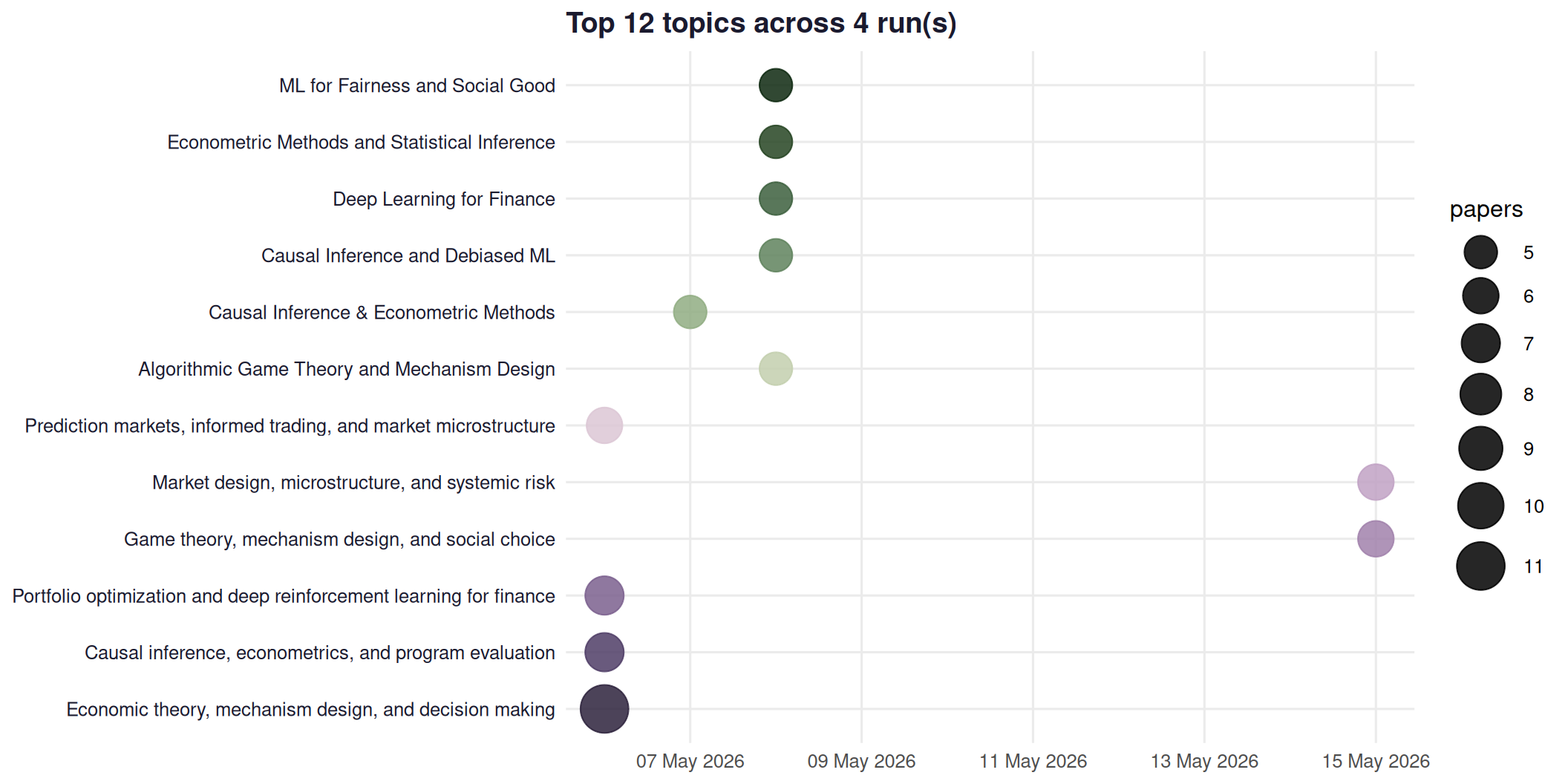
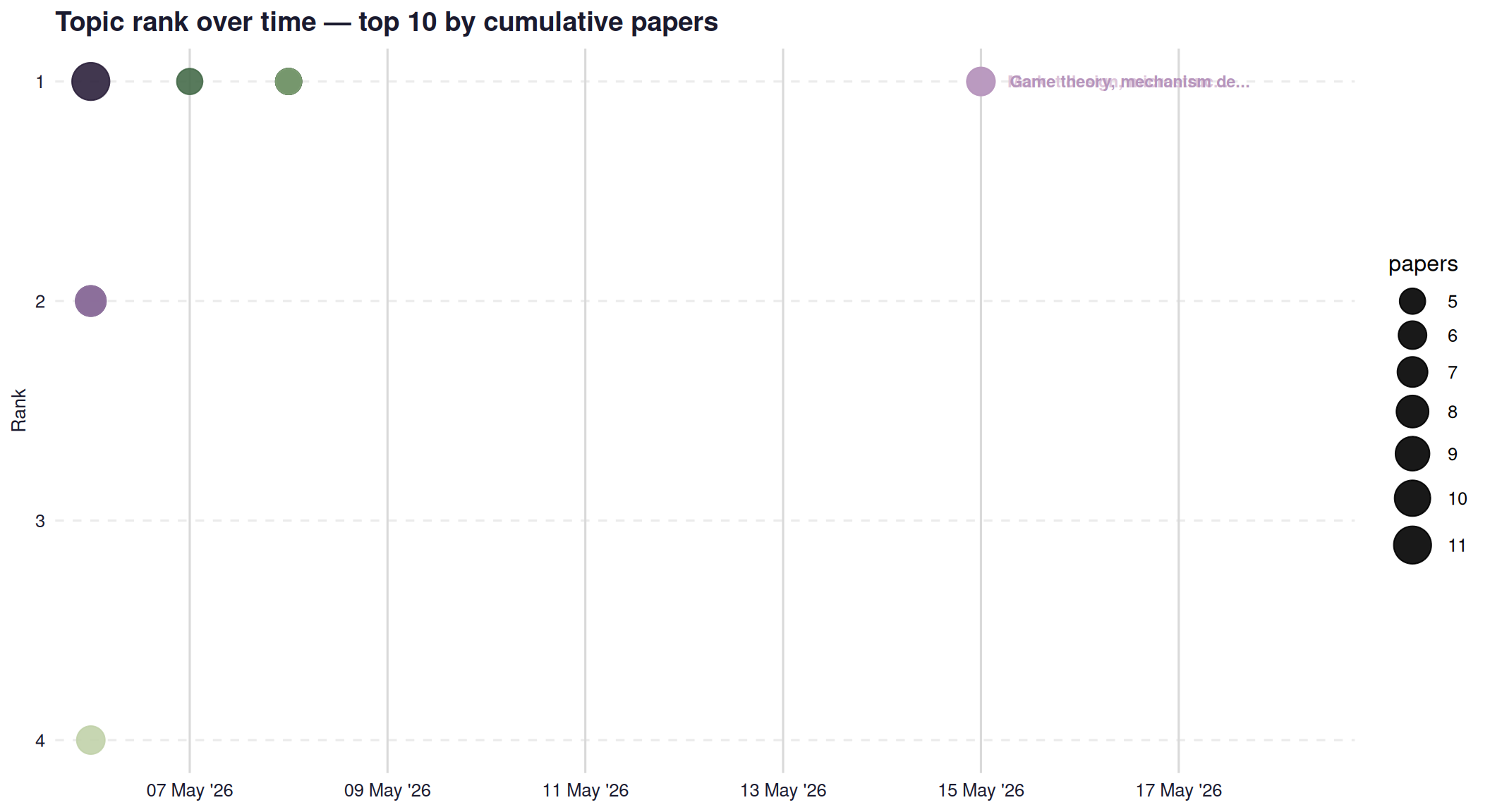
An interactive force-directed view of the topic landscape. Drag nodes, zoom, hover for details. Colors come from a Louvain community-detection pass on the co-occurrence graph.

Methodology & cadence

• Cadence — runs on the 1st and 15th of each month at 08:00 UTC via GitHub Actions (.github/workflows/ssrn-research.yml). Manual triggers via workflow_dispatch.
• Phase A (deterministic) — three arXiv queries, one per bucket, each returning the most-recent 80 candidates filtered to the last 14 days.
• Phase B (Claude Haiku tool-use) — picks the top-5 per bucket and clusters all candidates into 5–10 named topics. Edges are not emitted by the model — they’re computed from paper_ids intersections to guarantee consistency.
• Snapshots — one JSON per run in ssrn-research/snapshots/. Page reads them all on every render.

Last 8 runs:

• 2026-06-15 — 73 candidates (data_science=26, finance=25, social_sciences=25), 10 topics
• 2026-07-01 — 75 candidates (n/a), 0 topics
• 2026-07-15 — 73 candidates (data_science=25, finance=25, social_sciences=26), 10 topics
• 2026-08-01 — 70 candidates (n/a), 0 topics
• 2026-08-15 — 73 candidates (data_science=26, finance=25, social_sciences=25), 10 topics
• 2026-09-01 — 75 candidates (data_science=26, finance=25, social_sciences=25), 16 topics
• 2026-10-01 — 74 candidates (data_science=26, finance=25, social_sciences=25), 10 topics
• 2026-10-15 — 73 candidates (data_science=25, finance=25, social_sciences=25), 10 topics