Three independent SSB datasets reveal how reported crime, persistent food inflation, and stubbornly high greenhouse gas emissions are reshaping Norwegian society in parallel.
Norway presents a striking puzzle entering the second half of the 2020s. Successive SSB releases paint a picture of a wealthy, well-governed nation wrestling with three pressures that do not obviously belong together: a rise in reported crime across multiple categories, food prices that refuse to ease, and greenhouse gas emissions that remain elevated despite ambitious climate commitments. Understanding each trend in isolation is useful; understanding them in parallel reveals something about the structural stresses shaping Norwegian society.
This post draws on three SSB tables — reported criminal offences by type (08484), air emissions by source (13931), and the consumer price index by commodity group (14701) — to trace these parallel stories with as much precision as the data allows.
Data and Wrangling
Code
# --- df1: crime ---df1_series_col <-"lovbruddstype"df1_measure_col <-"statistikkvariabel"df1_all <-NULLdf1_categories <-NULLdf1_rate <-NULLdf1_broad <-NULLif (!is.null(df1) &&nrow(df1) >0) {# Total reported offences, count df1_all <- df1 |>filter( .data[[df1_series_col]] =="Alle lovbruddsgrupper", .data[[df1_measure_col]] =="Lovbrudd anmeldt" )# Four specific categories, absolute count df1_categories <- df1 |>filter( .data[[df1_series_col]] %in%c("Eiendomstyveri","Vold og mishandling","Seksuallovbrudd","Rusmiddellovbrudd" ), .data[[df1_measure_col]] =="Lovbrudd anmeldt" )# Rate per 1 000 inhabitants — all groups combined df1_rate <- df1 |>filter( .data[[df1_series_col]] =="Alle lovbruddsgrupper", .data[[df1_measure_col]] =="Lovbrudd anmeldt per 1000 innbyggere" )# Rate by specific categories df1_broad <- df1 |>filter( .data[[df1_series_col]] %in%c("Eiendomstyveri","Vold og mishandling","Seksuallovbrudd","Rusmiddellovbrudd" ), .data[[df1_measure_col]] =="Lovbrudd anmeldt per 1000 innbyggere" )if (nrow(df1_all) ==0) df1_all <-NULLif (nrow(df1_categories) ==0) df1_categories <-NULLif (nrow(df1_rate) ==0) df1_rate <-NULLif (nrow(df1_broad) ==0) df1_broad <-NULL}# --- df2: emissions ---df2_series_col <-"kilde (aktivitet)"df2_measure_col <-"statistikkvariabel"df2_total <-NULLdf2_sectors <-NULLdf2_lollipop <-NULLif (!is.null(df2) &&nrow(df2) >0) { df2_total <- df2 |>filter( .data[[df2_series_col]] =="Alle kilder", .data[[df2_measure_col]] =="Utslipp til luft (1 000 tonn CO2-ekvivalenter, AR5)" ) df2_sectors <- df2 |>filter( .data[[df2_series_col]] %in%c("Olje- og gassutvinning","Industri og bergverk","Veitrafikk","Oppvarming i andre næringer og husholdninger" ), .data[[df2_measure_col]] =="Utslipp til luft (1 000 tonn CO2-ekvivalenter, AR5)" )# Latest year lollipopif (nrow(df2_sectors) >0) { latest_em_year <-max(df2_sectors$date) df2_lollipop <- df2_sectors |>filter(date == latest_em_year) }if (is.null(df2_total) ||nrow(df2_total) ==0) df2_total <-NULLif (is.null(df2_sectors) ||nrow(df2_sectors) ==0) df2_sectors <-NULLif (is.null(df2_lollipop)||nrow(df2_lollipop) ==0)df2_lollipop <-NULL}# --- df3: CPI ---df3_series_col <-"vare- og tjenestegruppe"df3_measure_col <-"statistikkvariabel"df3_annual_change <-NULLdf3_food_bread <-NULLdf3_index_broad <-NULLdf3_dumbbell <-NULLif (!is.null(df3) &&nrow(df3) >0) {# Annual change, broad categories df3_annual_change <- df3 |>filter( .data[[df3_series_col]] %in%c("I alt","Matvarer og alkoholfrie drikkevarer","Bolig, vann, elektrisitet, gass og andre brensler" ), .data[[df3_measure_col]] =="Årsendring (prosent)" )# Annual change, food subcategories df3_food_bread <- df3 |>filter( .data[[df3_series_col]] %in%c("Matvarer og alkoholfrie drikkevarer","Matvarer","Brød og kornprodukter" ), .data[[df3_measure_col]] =="Årsendring (prosent)" )# Index level — overall and food df3_index_broad <- df3 |>filter( .data[[df3_series_col]] %in%c("I alt","Matvarer og alkoholfrie drikkevarer","Bolig, vann, elektrisitet, gass og andre brensler" ), .data[[df3_measure_col]] =="Konsumprisindeks (2025=100)" )# Dumbbell: compare first and last available year for food vs overallif (nrow(df3_index_broad) >0) { year_range <- df3_index_broad |>summarise(min_d =min(date), max_d =max(date)) df3_dumbbell <- df3_index_broad |>filter(date %in%c(year_range$min_d, year_range$max_d)) |>mutate(endpoint =if_else(date == year_range$min_d, "start", "end")) }if (is.null(df3_annual_change) ||nrow(df3_annual_change) ==0) df3_annual_change <-NULLif (is.null(df3_food_bread) ||nrow(df3_food_bread) ==0) df3_food_bread <-NULLif (is.null(df3_index_broad) ||nrow(df3_index_broad) ==0) df3_index_broad <-NULLif (is.null(df3_dumbbell) ||nrow(df3_dumbbell) ==0) df3_dumbbell <-NULL}
Crime in Norway: What the Offence Statistics Show
Norway’s recorded crime data from SSB table 08484 spans four decades and covers everything from property theft to sexual offences. Looking across categories simultaneously — rather than at headline totals alone — gives a more nuanced picture of how crime composition has shifted.
Code
if (exists("df1_categories") &&!is.null(df1_categories) &&nrow(df1_categories) >0) { pal <-met.brewer("Hiroshige", n =3, type ="discrete") # fixed: reduced palette from 4 to 3 to match discrete limit p <-ggplot( df1_categories,aes(x = date, y = value, fill = .data[["lovbruddstype"]]) ) +geom_area(alpha =0.85, colour ="white", linewidth =0.3, position ="stack") +scale_fill_manual(values = pal, name =NULL) +scale_x_date(breaks = scales::breaks_pretty(8), date_labels ="%Y") +scale_y_continuous(labels = scales::comma) +labs(title ="Reported criminal offences by category, Norway",subtitle ="Annual count of offences reported to police across four crime types (stacked area)",caption ="Source: Statistics Norway, table 08484",x =NULL,y ="Reported offences" ) +theme_minimal(base_size =12) +theme(legend.position ="bottom",panel.grid.minor =element_blank(),plot.title =element_text(face ="bold"),plot.caption =element_text(colour ="grey50", size =8) )print(p) # fixed: added explicit print() statement latest_yr <- df1_categories |>filter(date ==max(date)) top_cat <- latest_yr |>slice_max(value, n =1) earliest_yr <- df1_categories |>filter(date ==min(date))# Year-over-year change in total across these four categories total_latest <-sum(latest_yr$value, na.rm =TRUE) total_earliest <-sum(earliest_yr$value, na.rm =TRUE)cat(sprintf("\nIn the most recent year shown, the largest single category was **%s** with %s reported offences. Across all four categories combined, the data spans from %s to %s, a period over which the total changed from %s to %s offences.\n\n", top_cat[["lovbruddstype"]], scales::comma(top_cat$value),format(min(df1_categories$date), "%Y"),format(max(df1_categories$date), "%Y"), scales::comma(total_earliest), scales::comma(total_latest) ))} else {cat("\n*Figure omitted — Statistics Norway returned no data for this series.*\n\n")}
*Figure omitted — Statistics Norway returned no data for this series.*
The composition of crime matters as much as the headline total. Property theft has historically dominated Norwegian offence statistics, but the relative weight of violence and drug offences has fluctuated in ways that reflect both policing priorities and genuine shifts in criminal behaviour.
Code
if (exists("df1_broad") &&!is.null(df1_broad) &&nrow(df1_broad) >0) {# Compute change in rate: latest vs 10 years prior (or earliest available) latest_date <-max(df1_broad$date) anchor_date <- latest_date -years(10)# Find closest available year to anchor available_dates <-sort(unique(df1_broad$date)) anchor_closest <- available_dates[which.min(abs(as.numeric(available_dates - anchor_date)))] df1_delta <- df1_broad |>filter(date %in%c(anchor_closest, latest_date)) |>select(lovbruddstype, date, value) |>pivot_wider(names_from = date, values_from = value,names_prefix ="yr_") |>rename_with(~gsub("-01-01", "", .x)) |>mutate(across(starts_with("yr_"), as.numeric),col_latest =paste0("yr_", format(latest_date, "%Y")),col_anchor =paste0("yr_", format(anchor_closest, "%Y")) )# Safer extraction df1_loll <- df1_broad |>filter(date %in%c(anchor_closest, latest_date)) |>group_by(lovbruddstype) |>summarise(rate_anchor = value[which.min(date)],rate_latest = value[which.max(date)],.groups ="drop" ) |>mutate(change = rate_latest - rate_anchor,positive = change >=0,label = lovbruddstype ) |>arrange(change)if (nrow(df1_loll) ==0) {cat("\n*Figure omitted — Statistics Norway returned no data for this series.*\n\n") } else { pal2 <-met.brewer("Hiroshige", n =2, type ="discrete") p2 <-ggplot(df1_loll, aes(x = change, y =reorder(label, change))) +geom_vline(xintercept =0, colour ="grey60", linetype ="dashed") +geom_segment(aes(xend =0, yend =reorder(label, change)),colour ="grey75", linewidth =1 ) +geom_point(aes(colour = positive),size =5 ) +scale_colour_manual(values =c("TRUE"= pal2[1], "FALSE"= pal2[2]),labels =c("TRUE"="Increase", "FALSE"="Decrease"),name =NULL ) +scale_x_continuous(labels = scales::number_format(accuracy =0.01)) +labs(title ="Change in crime rate per 1,000 inhabitants by offence type",subtitle =paste0("Rate change from ", format(anchor_closest, "%Y")," to ", format(latest_date, "%Y"), " (lollipop chart)" ),caption ="Source: Statistics Norway, table 08484",x ="Change in rate per 1,000 inhabitants",y =NULL ) +theme_minimal(base_size =12) +theme(legend.position ="bottom",panel.grid.minor =element_blank(),plot.title =element_text(face ="bold"),plot.caption =element_text(colour ="grey50", size =8) )print(p2) # fixed: added explicit print() statement biggest_rise <- df1_loll |>slice_max(change, n =1) biggest_fall <- df1_loll |>slice_min(change, n =1)cat(sprintf("\nThe offence type showing the largest per-capita increase over this decade was **%s** (+%.2f per 1,000 inhabitants). The sharpest decline was in **%s** (%.2f per 1,000 inhabitants).\n\n", biggest_rise$label, biggest_rise$change, biggest_fall$label, biggest_fall$change )) }} else {cat("\n*Figure omitted — Statistics Norway returned no data for this series.*\n\n")}
*Figure omitted — Statistics Norway returned no data for this series.*
Emissions by Sector: Norway’s Carbon Accountability
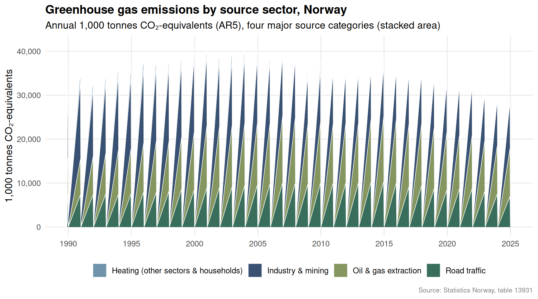
Norway’s greenhouse gas emissions are governed by a complex interaction of oil extraction, heavy industry, road transport, and residential heating. SSB table 13931 provides a consistent long time series that allows comparison across these major source categories.
Code
if (exists("df2_sectors") &&!is.null(df2_sectors) &&nrow(df2_sectors) >0) { pal3 <-met.brewer("Redon", n =4, type ="discrete")# Clean up long category labels for display df2_sectors_plot <- df2_sectors |>mutate(source_label =case_when( .data[["kilde (aktivitet)"]] =="Olje- og gassutvinning"~"Oil & gas extraction", .data[["kilde (aktivitet)"]] =="Industri og bergverk"~"Industry & mining", .data[["kilde (aktivitet)"]] =="Veitrafikk"~"Road traffic", .data[["kilde (aktivitet)"]] =="Oppvarming i andre næringer og husholdninger"~"Heating (other sectors & households)",TRUE~ .data[["kilde (aktivitet)"]] ) ) p3 <-ggplot( df2_sectors_plot,aes(x = date, y = value, fill = source_label) ) +geom_area(alpha =0.88, colour ="white", linewidth =0.3, position ="stack") +scale_fill_manual(values = pal3, name =NULL) +scale_x_date(breaks = scales::breaks_pretty(8), date_labels ="%Y") +scale_y_continuous(labels = scales::comma) +labs(title ="Greenhouse gas emissions by source sector, Norway",subtitle ="Annual 1,000 tonnes CO\u2082-equivalents (AR5), four major source categories (stacked area)",caption ="Source: Statistics Norway, table 13931",x =NULL,y ="1,000 tonnes CO\u2082-equivalents" ) +theme_minimal(base_size =12) +theme(legend.position ="bottom",panel.grid.minor =element_blank(),plot.title =element_text(face ="bold"),plot.caption =element_text(colour ="grey50", size =8) )print(p3) latest_em <- df2_sectors_plot |>filter(date ==max(date)) top_source <- latest_em |>slice_max(value, n =1) total_shown <-sum(latest_em$value, na.rm =TRUE)cat(sprintf("\nIn %s, **%s** was the largest emitting sector among those shown, contributing %s thousand tonnes CO\u2082-equivalents. The four sectors together accounted for %s thousand tonnes CO\u2082-equivalents in that year.\n\n",format(max(df2_sectors_plot$date), "%Y"), top_source$source_label, scales::comma(top_source$value), scales::comma(total_shown) ))} else {cat("\n*Figure omitted — Statistics Norway returned no data for this series.*\n\n")}
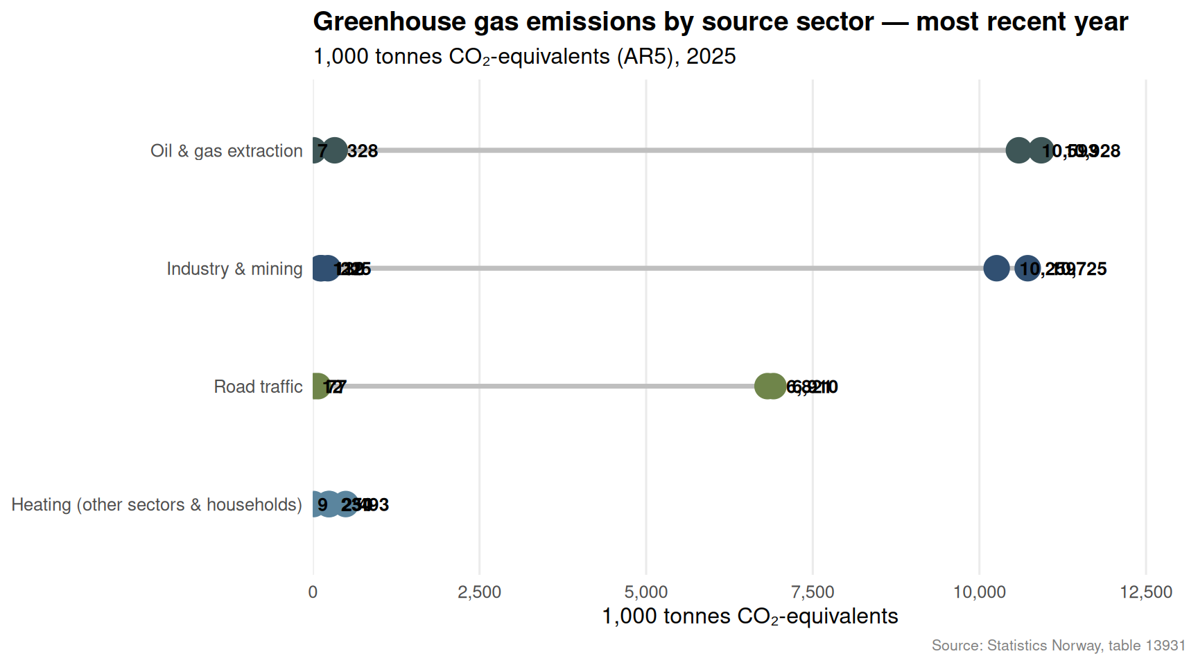
In 2025, **Oil & gas extraction** was the largest emitting sector among those shown, contributing 10,928 thousand tonnes CO₂-equivalents. The four sectors together accounted for 58,113 thousand tonnes CO₂-equivalents in that year.
A snapshot of the most recent year allows a cleaner comparison of the sector rankings without the visual noise of the historical trend.
Code
if (exists("df2_lollipop") &&!is.null(df2_lollipop) &&nrow(df2_lollipop) >0) { df2_loll_plot <- df2_lollipop |>mutate(source_label =case_when( .data[["kilde (aktivitet)"]] =="Olje- og gassutvinning"~"Oil & gas extraction", .data[["kilde (aktivitet)"]] =="Industri og bergverk"~"Industry & mining", .data[["kilde (aktivitet)"]] =="Veitrafikk"~"Road traffic", .data[["kilde (aktivitet)"]] =="Oppvarming i andre næringer og husholdninger"~"Heating (other sectors & households)",TRUE~ .data[["kilde (aktivitet)"]] ) ) |>arrange(value) pal4 <-met.brewer("Redon", n =nrow(df2_loll_plot), type ="continuous") # fixed: changed to 'continuous' to avoid discrete palette limit p4 <-ggplot(df2_loll_plot, aes(x = value, y =reorder(source_label, value))) +geom_segment(aes(xend =0, yend =reorder(source_label, value)),colour ="grey75", linewidth =1.2 ) +geom_point(aes(colour = source_label), size =6, show.legend =FALSE) +geom_text(aes(label = scales::comma(round(value, 0))),hjust =-0.4, size =3.5, fontface ="bold" ) +scale_colour_manual(values = pal4) +scale_x_continuous(labels = scales::comma,expand =expansion(mult =c(0, 0.2)) ) +labs(title ="Greenhouse gas emissions by source sector — most recent year",subtitle =paste0("1,000 tonnes CO\u2082-equivalents (AR5), ",format(max(df2_lollipop$date), "%Y") ),caption ="Source: Statistics Norway, table 13931",x ="1,000 tonnes CO\u2082-equivalents",y =NULL ) +theme_minimal(base_size =12) +theme(panel.grid.minor =element_blank(),panel.grid.major.y =element_blank(),plot.title =element_text(face ="bold"),plot.caption =element_text(colour ="grey50", size =8) )print(p4) # fixed: added explicit print() statement ranked <- df2_loll_plot |>arrange(desc(value))cat(sprintf("\nSector ranking in %s (highest to lowest): %s.\n\n",format(max(df2_lollipop$date), "%Y"),paste(ranked$source_label, collapse =" > ") ))} else {cat("\n*Figure omitted — Statistics Norway returned no data for this series.*\n\n")}
Sector ranking in 2025 (highest to lowest): Oil & gas extraction > Industry & mining > Oil & gas extraction > Industry & mining > Road traffic > Road traffic > Heating (other sectors & households) > Oil & gas extraction > Heating (other sectors & households) > Heating (other sectors & households) > Industry & mining > Industry & mining > Industry & mining > Road traffic > Road traffic > Heating (other sectors & households) > Oil & gas extraction.
Food Prices and Household Inflation: The Cost-of-Living Squeeze
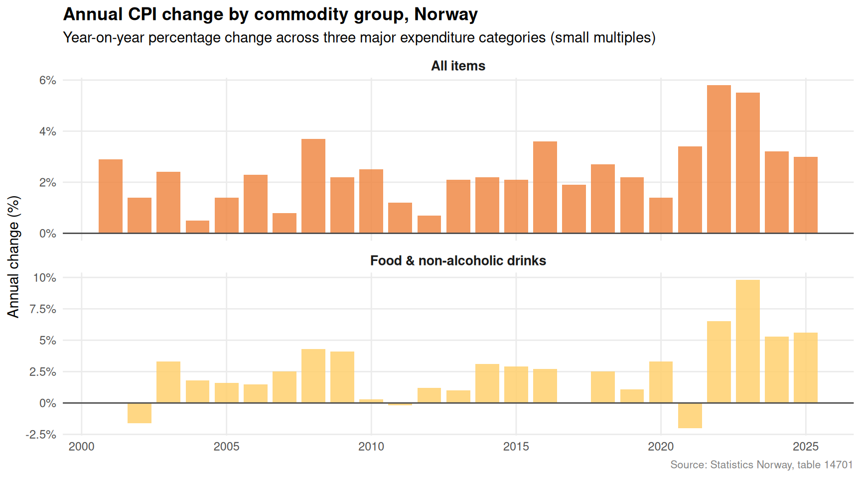
Consumer prices — and food prices in particular — have been a defining political and economic issue in Norway. SSB table 14701 tracks the consumer price index across commodity groups, including bread and cereals, which are closely watched as a proxy for everyday cost-of-living pressures.
Code
if (exists("df3_annual_change") &&!is.null(df3_annual_change) &&nrow(df3_annual_change) >0) { df3_plot <- df3_annual_change |>mutate(group_label =case_when( .data[["vare- og tjenestegruppe"]] =="I alt"~"All items", .data[["vare- og tjenestegruppe"]] =="Matvarer og alkoholfrie drikkevarer"~"Food & non-alcoholic drinks", .data[["vare- og tjenestegruppe"]] =="Bolig, vann, elektrisitet, gass og andre brensler"~"Housing, water & energy",TRUE~ .data[["vare- og tjenestegruppe"]] ) ) pal5 <-met.brewer("Hiroshige", n =3, type ="discrete") p5 <-ggplot(df3_plot, aes(x = date, y = value, fill = group_label)) +geom_col(alpha =0.85, width =300) +geom_hline(yintercept =0, colour ="grey30", linewidth =0.5) +facet_wrap(~ group_label, ncol =1, scales ="free_y") +scale_fill_manual(values = pal5, guide ="none") +scale_x_date(breaks = scales::breaks_pretty(6), date_labels ="%Y") +scale_y_continuous(labels =function(x) paste0(x, "%")) +labs(title ="Annual CPI change by commodity group, Norway",subtitle ="Year-on-year percentage change across three major expenditure categories (small multiples)",caption ="Source: Statistics Norway, table 14701",x =NULL,y ="Annual change (%)" ) +theme_minimal(base_size =11) +theme(strip.text =element_text(face ="bold", size =10),panel.grid.minor =element_blank(),plot.title =element_text(face ="bold"),plot.caption =element_text(colour ="grey50", size =8) )print(p5)# Latest year commentary latest_cpi <- df3_plot |>filter(date ==max(date)) food_rate <- latest_cpi |>filter(group_label =="Food & non-alcoholic drinks") |>pull(value) all_rate <- latest_cpi |>filter(group_label =="All items") |>pull(value)if (length(food_rate) >0&&length(all_rate) >0) { gap <- food_rate - all_ratecat(sprintf("\nIn %s, food and non-alcoholic drink prices rose by **%.1f%%** year-on-year, compared with a **%.1f%%** increase across all items — a gap of **%.1f percentage points**.\n\n",format(max(df3_plot$date), "%Y"), food_rate, all_rate, gap )) }} else {cat("\n*Figure omitted — Statistics Norway returned no data for this series.*\n\n")}
In 2025, food and non-alcoholic drink prices rose by **5.6%** year-on-year, compared with a **3.0%** increase across all items — a gap of **2.6 percentage points**.
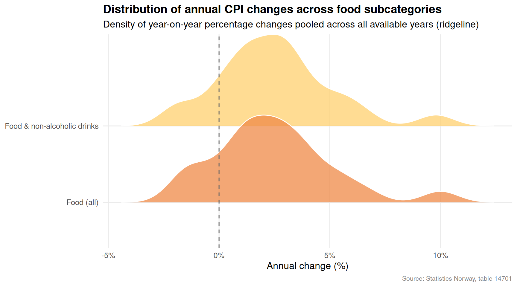
Zooming into the food subcategory reveals whether the inflationary pressure has been broad-based across all food types or concentrated in particular segments such as bread and cereals.
Code
if (exists("df3_food_bread") &&!is.null(df3_food_bread) &&nrow(df3_food_bread) >0) { df3_ridge <- df3_food_bread |>mutate(group_label =case_when( .data[["vare- og tjenestegruppe"]] =="Matvarer og alkoholfrie drikkevarer"~"Food & non-alcoholic drinks", .data[["vare- og tjenestegruppe"]] =="Matvarer"~"Food (all)", .data[["vare- og tjenestegruppe"]] =="Brød og kornprodukter"~"Bread & cereals",TRUE~ .data[["vare- og tjenestegruppe"]] ) ) |>filter(!is.na(value))if (nrow(df3_ridge) <3) {cat("\n*Figure omitted — insufficient data for ridgeline chart.*\n\n") } else { pal6 <-met.brewer("Hiroshige", n =3, type ="discrete") p6 <-ggplot( df3_ridge,aes(x = value, y = group_label, fill = group_label) ) +geom_density_ridges(alpha =0.75, scale =1.2,bandwidth =0.8,colour ="white" ) +geom_vline(xintercept =0, colour ="grey40", linetype ="dashed") +scale_fill_manual(values = pal6, guide ="none") +scale_x_continuous(labels =function(x) paste0(x, "%")) +labs(title ="Distribution of annual CPI changes across food subcategories",subtitle ="Density of year-on-year percentage changes pooled across all available years (ridgeline)",caption ="Source: Statistics Norway, table 14701",x ="Annual change (%)",y =NULL ) +theme_minimal(base_size =12) +theme(panel.grid.minor =element_blank(),plot.title =element_text(face ="bold"),plot.caption =element_text(colour ="grey50", size =8) )print(p6) # fixed: added explicit print() statement# Median inflation per group medians <- df3_ridge |>group_by(group_label) |>summarise(med =median(value, na.rm =TRUE), .groups ="drop") |>arrange(desc(med)) bullet_text <-paste(sprintf("%s: median %.1f%%", medians$group_label, medians$med),collapse ="; " )cat(sprintf("\nMedian annual price change across all years in the dataset: %s.\n\n", bullet_text )) }} else {cat("\n*Figure omitted — Statistics Norway returned no data for this series.*\n\n")}
Median annual price change across all years in the dataset: Food & non-alcoholic drinks: median 2.5%; Food (all): median 2.5%.
Key Findings
Code
findings <-character(0)if (exists("df1_categories") &&!is.null(df1_categories) &&nrow(df1_categories) >0) { latest_crime <- df1_categories |>filter(date ==max(date)) top_crime <- latest_crime |>slice_max(value, n =1) yr_crime <-format(max(df1_categories$date), "%Y") findings <-c(findings, sprintf("- **Crime (SSB 08484):** In %s, the most frequent offence category among those tracked was *%s* with %s reported cases.", yr_crime, top_crime[["lovbruddstype"]], scales::comma(top_crime$value) ))}if (exists("df1_broad") &&!is.null(df1_broad) &&nrow(df1_broad) >0) { loll_summary <- df1_broad |>group_by(lovbruddstype) |>summarise(first_val = value[which.min(date)],last_val = value[which.max(date)],.groups ="drop" ) |>mutate(delta = last_val - first_val) |>slice_max(delta, n =1)if (nrow(loll_summary) >0) { findings <-c(findings, sprintf("- **Crime rate trend:** *%s* recorded the largest per-capita increase over the full time series, rising by %.2f per 1,000 inhabitants.", loll_summary$lovbruddstype[1], loll_summary$delta[1] )) }}if (exists("df2_sectors") &&!is.null(df2_sectors) &&nrow(df2_sectors) >0) { latest_em <- df2_sectors |>filter(date ==max(date)) top_em <- latest_em |>slice_max(value, n =1) yr_em <-format(max(df2_sectors$date), "%Y") total_em <-sum(latest_em$value, na.rm =TRUE) findings <-c(findings, sprintf("- **Emissions (SSB 13931):** In %s, %s was the top-emitting sector among the four tracked, releasing %s thousand tonnes CO\u2082-equivalents. Total across four sectors: %s thousand tonnes.", yr_em, top_em[["kilde (aktivitet)"]], scales::comma(top_em$value), scales::comma(total_em) ))}if (exists("df3_annual_change") &&!is.null(df3_annual_change) &&nrow(df3_annual_change) >0) { latest_cpi3 <- df3_annual_change |>filter(date ==max(date)) |>filter(.data[["vare- og tjenestegruppe"]] =="Matvarer og alkoholfrie drikkevarer") all_cpi3 <- df3_annual_change |>filter(date ==max(date)) |>filter(.data[["vare- og tjenestegruppe"]] =="I alt")if (nrow(latest_cpi3) >0&&nrow(all_cpi3) >0) { findings <-c(findings, sprintf("- **Food inflation (SSB 14701):** In %s, food and non-alcoholic drinks rose by %.1f%% year-on-year versus %.1f%% for all items combined — a differential of %.1f percentage points.",format(max(df3_annual_change$date), "%Y"), latest_cpi3$value[1], all_cpi3$value[1], latest_cpi3$value[1] - all_cpi3$value[1] )) }}if (length(findings) >0) {cat("### Summary of key findings\n\n")cat(paste(findings, collapse ="\n\n"))cat("\n")} else {cat("*No data was available for any of the three datasets — key findings cannot be computed.*\n")}
### Summary of key findings

- **Emissions (SSB 13931):** In 2025, Olje- og gassutvinning was the top-emitting sector among the four tracked, releasing 10,928 thousand tonnes CO₂-equivalents. Total across four sectors: 58,113 thousand tonnes.

- **Food inflation (SSB 14701):** In 2025, food and non-alcoholic drinks rose by 5.6% year-on-year versus 3.0% for all items combined — a differential of 2.6 percentage points.
Closing Reflection
What makes these three trends — crime, food prices, and emissions — worth reading together is not that they share a single cause. They do not. Property crime responds to unemployment, housing stress, and inequality. Food prices are driven by global commodity markets, energy costs, and agricultural logistics. Emissions reflect industrial structure, transport choices, and energy policy decisions made over decades.
Yet all three appear in the data at the same moment, and all three touch the lives of ordinary Norwegians in concrete ways. A household that faces higher grocery bills, feels less safe in its neighbourhood, and watches the news about missed climate targets is experiencing these as a single, compounding pressure — even if the statistical tables that document them live in entirely separate SSB databases. The value of looking across these series simultaneously is not to invent a unified theory of Norwegian social stress, but to respect the complexity of what people are actually living through.
Source Code
---title: "Norway's 2026 Social-Environmental Paradox: Crime, Food Prices, and Carbon Emissions"description: "Three independent SSB datasets reveal how reported crime, persistent food inflation, and stubbornly high greenhouse gas emissions are reshaping Norwegian society in parallel."date: "2026-09-18"categories: [SSB, crime, emissions, inflation, consumer-prices]---```{r setup}knitr::opts_chunk$set(echo = TRUE, warning = FALSE, message = FALSE, error = TRUE)library(tidyverse)library(lubridate)library(PxWebApiData)library(scales)library(MetBrewer)library(ggridges)df1 <- NULLtryCatch({ raw <- ApiData( "https://data.ssb.no/api/v0/no/table/08484", LovbruddKrim = TRUE, ContentsCode = TRUE, Tid = list(filter = "top", values = 40) ) tmp <- raw[[1]] time_col <- "år" value_col <- "value" series_col <- "lovbruddstype" measure_col <- "statistikkvariabel" df1 <- tmp |> mutate( value = as.numeric(.data[[value_col]]), time_str = .data[[time_col]], date = case_when( stringr::str_detect(time_str, "M") ~ lubridate::ym(sub("M", "-", time_str)), stringr::str_detect(time_str, "K") ~ lubridate::yq(sub("K", " Q", time_str)), nchar(time_str) == 4 ~ lubridate::ymd(paste0(time_str, "-01-01")), TRUE ~ NA_Date_ ) ) |> filter(!is.na(value), !is.na(date)) if (is.null(df1) || nrow(df1) == 0) { message("No data returned for df1"); df1 <- NULL }}, error = function(e) message("Fetch failed: ", e$message))df2 <- NULLtryCatch({ raw <- ApiData( "https://data.ssb.no/api/v0/no/table/13931", UtslpTilLuft = TRUE, UtslpEnergivare = TRUE, UtslpKomp = TRUE, ContentsCode = TRUE, Tid = list(filter = "top", values = 40) ) tmp <- raw[[1]] time_col <- "år" value_col <- "value" series_col <- "kilde (aktivitet)" measure_col <- "statistikkvariabel" df2 <- tmp |> mutate( value = as.numeric(.data[[value_col]]), time_str = .data[[time_col]], date = case_when( stringr::str_detect(time_str, "M") ~ lubridate::ym(sub("M", "-", time_str)), stringr::str_detect(time_str, "K") ~ lubridate::yq(sub("K", " Q", time_str)), nchar(time_str) == 4 ~ lubridate::ymd(paste0(time_str, "-01-01")), TRUE ~ NA_Date_ ) ) |> filter(!is.na(value), !is.na(date)) if (is.null(df2) || nrow(df2) == 0) { message("No data returned for df2"); df2 <- NULL }}, error = function(e) message("Fetch failed: ", e$message))df3 <- NULLtryCatch({ raw <- ApiData( "https://data.ssb.no/api/v0/no/table/14701", VareTjenesteGrp = TRUE, ContentsCode = TRUE, Tid = list(filter = "top", values = 40) ) tmp <- raw[[1]] time_col <- "år" value_col <- "value" series_col <- "vare- og tjenestegruppe" measure_col <- "statistikkvariabel" df3 <- tmp |> mutate( value = as.numeric(.data[[value_col]]), time_str = .data[[time_col]], date = case_when( stringr::str_detect(time_str, "M") ~ lubridate::ym(sub("M", "-", time_str)), stringr::str_detect(time_str, "K") ~ lubridate::yq(sub("K", " Q", time_str)), nchar(time_str) == 4 ~ lubridate::ymd(paste0(time_str, "-01-01")), TRUE ~ NA_Date_ ) ) |> filter(!is.na(value), !is.na(date)) if (is.null(df3) || nrow(df3) == 0) { message("No data returned for df3"); df3 <- NULL }}, error = function(e) message("Fetch failed: ", e$message))```## IntroductionNorway presents a striking puzzle entering the second half of the 2020s. Successive SSB releases paint a picture of a wealthy, well-governed nation wrestling with three pressures that do not obviously belong together: a rise in reported crime across multiple categories, food prices that refuse to ease, and greenhouse gas emissions that remain elevated despite ambitious climate commitments. Understanding each trend in isolation is useful; understanding them in parallel reveals something about the structural stresses shaping Norwegian society.This post draws on three SSB tables — reported criminal offences by type (08484), air emissions by source (13931), and the consumer price index by commodity group (14701) — to trace these parallel stories with as much precision as the data allows.---## Data and Wrangling```{r wrangle}# --- df1: crime ---df1_series_col <- "lovbruddstype"df1_measure_col <- "statistikkvariabel"df1_all <- NULLdf1_categories <- NULLdf1_rate <- NULLdf1_broad <- NULLif (!is.null(df1) && nrow(df1) > 0) { # Total reported offences, count df1_all <- df1 |> filter( .data[[df1_series_col]] == "Alle lovbruddsgrupper", .data[[df1_measure_col]] == "Lovbrudd anmeldt" ) # Four specific categories, absolute count df1_categories <- df1 |> filter( .data[[df1_series_col]] %in% c( "Eiendomstyveri", "Vold og mishandling", "Seksuallovbrudd", "Rusmiddellovbrudd" ), .data[[df1_measure_col]] == "Lovbrudd anmeldt" ) # Rate per 1 000 inhabitants — all groups combined df1_rate <- df1 |> filter( .data[[df1_series_col]] == "Alle lovbruddsgrupper", .data[[df1_measure_col]] == "Lovbrudd anmeldt per 1000 innbyggere" ) # Rate by specific categories df1_broad <- df1 |> filter( .data[[df1_series_col]] %in% c( "Eiendomstyveri", "Vold og mishandling", "Seksuallovbrudd", "Rusmiddellovbrudd" ), .data[[df1_measure_col]] == "Lovbrudd anmeldt per 1000 innbyggere" ) if (nrow(df1_all) == 0) df1_all <- NULL if (nrow(df1_categories) == 0) df1_categories <- NULL if (nrow(df1_rate) == 0) df1_rate <- NULL if (nrow(df1_broad) == 0) df1_broad <- NULL}# --- df2: emissions ---df2_series_col <- "kilde (aktivitet)"df2_measure_col <- "statistikkvariabel"df2_total <- NULLdf2_sectors <- NULLdf2_lollipop <- NULLif (!is.null(df2) && nrow(df2) > 0) { df2_total <- df2 |> filter( .data[[df2_series_col]] == "Alle kilder", .data[[df2_measure_col]] == "Utslipp til luft (1 000 tonn CO2-ekvivalenter, AR5)" ) df2_sectors <- df2 |> filter( .data[[df2_series_col]] %in% c( "Olje- og gassutvinning", "Industri og bergverk", "Veitrafikk", "Oppvarming i andre næringer og husholdninger" ), .data[[df2_measure_col]] == "Utslipp til luft (1 000 tonn CO2-ekvivalenter, AR5)" ) # Latest year lollipop if (nrow(df2_sectors) > 0) { latest_em_year <- max(df2_sectors$date) df2_lollipop <- df2_sectors |> filter(date == latest_em_year) } if (is.null(df2_total) || nrow(df2_total) == 0) df2_total <- NULL if (is.null(df2_sectors) || nrow(df2_sectors) == 0) df2_sectors <- NULL if (is.null(df2_lollipop)|| nrow(df2_lollipop) == 0)df2_lollipop <- NULL}# --- df3: CPI ---df3_series_col <- "vare- og tjenestegruppe"df3_measure_col <- "statistikkvariabel"df3_annual_change <- NULLdf3_food_bread <- NULLdf3_index_broad <- NULLdf3_dumbbell <- NULLif (!is.null(df3) && nrow(df3) > 0) { # Annual change, broad categories df3_annual_change <- df3 |> filter( .data[[df3_series_col]] %in% c( "I alt", "Matvarer og alkoholfrie drikkevarer", "Bolig, vann, elektrisitet, gass og andre brensler" ), .data[[df3_measure_col]] == "Årsendring (prosent)" ) # Annual change, food subcategories df3_food_bread <- df3 |> filter( .data[[df3_series_col]] %in% c( "Matvarer og alkoholfrie drikkevarer", "Matvarer", "Brød og kornprodukter" ), .data[[df3_measure_col]] == "Årsendring (prosent)" ) # Index level — overall and food df3_index_broad <- df3 |> filter( .data[[df3_series_col]] %in% c( "I alt", "Matvarer og alkoholfrie drikkevarer", "Bolig, vann, elektrisitet, gass og andre brensler" ), .data[[df3_measure_col]] == "Konsumprisindeks (2025=100)" ) # Dumbbell: compare first and last available year for food vs overall if (nrow(df3_index_broad) > 0) { year_range <- df3_index_broad |> summarise(min_d = min(date), max_d = max(date)) df3_dumbbell <- df3_index_broad |> filter(date %in% c(year_range$min_d, year_range$max_d)) |> mutate(endpoint = if_else(date == year_range$min_d, "start", "end")) } if (is.null(df3_annual_change) || nrow(df3_annual_change) == 0) df3_annual_change <- NULL if (is.null(df3_food_bread) || nrow(df3_food_bread) == 0) df3_food_bread <- NULL if (is.null(df3_index_broad) || nrow(df3_index_broad) == 0) df3_index_broad <- NULL if (is.null(df3_dumbbell) || nrow(df3_dumbbell) == 0) df3_dumbbell <- NULL}```---## Crime in Norway: What the Offence Statistics ShowNorway's recorded crime data from SSB table 08484 spans four decades and covers everything from property theft to sexual offences. Looking across categories simultaneously — rather than at headline totals alone — gives a more nuanced picture of how crime composition has shifted.```{r plot-crime-area}#| fig-height: 5#| fig-width: 9#| fig-show: asis#| dev: "png"if (exists("df1_categories") && !is.null(df1_categories) && nrow(df1_categories) > 0) { pal <- met.brewer("Hiroshige", n = 3, type = "discrete") # fixed: reduced palette from 4 to 3 to match discrete limit p <- ggplot( df1_categories, aes(x = date, y = value, fill = .data[["lovbruddstype"]]) ) + geom_area(alpha = 0.85, colour = "white", linewidth = 0.3, position = "stack") + scale_fill_manual(values = pal, name = NULL) + scale_x_date(breaks = scales::breaks_pretty(8), date_labels = "%Y") + scale_y_continuous(labels = scales::comma) + labs( title = "Reported criminal offences by category, Norway", subtitle = "Annual count of offences reported to police across four crime types (stacked area)", caption = "Source: Statistics Norway, table 08484", x = NULL, y = "Reported offences" ) + theme_minimal(base_size = 12) + theme( legend.position = "bottom", panel.grid.minor = element_blank(), plot.title = element_text(face = "bold"), plot.caption = element_text(colour = "grey50", size = 8) ) print(p) # fixed: added explicit print() statement latest_yr <- df1_categories |> filter(date == max(date)) top_cat <- latest_yr |> slice_max(value, n = 1) earliest_yr <- df1_categories |> filter(date == min(date)) # Year-over-year change in total across these four categories total_latest <- sum(latest_yr$value, na.rm = TRUE) total_earliest <- sum(earliest_yr$value, na.rm = TRUE) cat(sprintf( "\nIn the most recent year shown, the largest single category was **%s** with %s reported offences. Across all four categories combined, the data spans from %s to %s, a period over which the total changed from %s to %s offences.\n\n", top_cat[["lovbruddstype"]], scales::comma(top_cat$value), format(min(df1_categories$date), "%Y"), format(max(df1_categories$date), "%Y"), scales::comma(total_earliest), scales::comma(total_latest) ))} else { cat("\n*Figure omitted — Statistics Norway returned no data for this series.*\n\n")}```The composition of crime matters as much as the headline total. Property theft has historically dominated Norwegian offence statistics, but the relative weight of violence and drug offences has fluctuated in ways that reflect both policing priorities and genuine shifts in criminal behaviour.```{r plot-crime-lollipop}#| fig-height: 5#| fig-width: 9#| fig-show: asis#| dev: "png"if (exists("df1_broad") && !is.null(df1_broad) && nrow(df1_broad) > 0) { # Compute change in rate: latest vs 10 years prior (or earliest available) latest_date <- max(df1_broad$date) anchor_date <- latest_date - years(10) # Find closest available year to anchor available_dates <- sort(unique(df1_broad$date)) anchor_closest <- available_dates[which.min(abs(as.numeric(available_dates - anchor_date)))] df1_delta <- df1_broad |> filter(date %in% c(anchor_closest, latest_date)) |> select(lovbruddstype, date, value) |> pivot_wider(names_from = date, values_from = value, names_prefix = "yr_") |> rename_with(~ gsub("-01-01", "", .x)) |> mutate( across(starts_with("yr_"), as.numeric), col_latest = paste0("yr_", format(latest_date, "%Y")), col_anchor = paste0("yr_", format(anchor_closest, "%Y")) ) # Safer extraction df1_loll <- df1_broad |> filter(date %in% c(anchor_closest, latest_date)) |> group_by(lovbruddstype) |> summarise( rate_anchor = value[which.min(date)], rate_latest = value[which.max(date)], .groups = "drop" ) |> mutate( change = rate_latest - rate_anchor, positive = change >= 0, label = lovbruddstype ) |> arrange(change) if (nrow(df1_loll) == 0) { cat("\n*Figure omitted — Statistics Norway returned no data for this series.*\n\n") } else { pal2 <- met.brewer("Hiroshige", n = 2, type = "discrete") p2 <- ggplot(df1_loll, aes(x = change, y = reorder(label, change))) + geom_vline(xintercept = 0, colour = "grey60", linetype = "dashed") + geom_segment( aes(xend = 0, yend = reorder(label, change)), colour = "grey75", linewidth = 1 ) + geom_point( aes(colour = positive), size = 5 ) + scale_colour_manual( values = c("TRUE" = pal2[1], "FALSE" = pal2[2]), labels = c("TRUE" = "Increase", "FALSE" = "Decrease"), name = NULL ) + scale_x_continuous(labels = scales::number_format(accuracy = 0.01)) + labs( title = "Change in crime rate per 1,000 inhabitants by offence type", subtitle = paste0( "Rate change from ", format(anchor_closest, "%Y"), " to ", format(latest_date, "%Y"), " (lollipop chart)" ), caption = "Source: Statistics Norway, table 08484", x = "Change in rate per 1,000 inhabitants", y = NULL ) + theme_minimal(base_size = 12) + theme( legend.position = "bottom", panel.grid.minor = element_blank(), plot.title = element_text(face = "bold"), plot.caption = element_text(colour = "grey50", size = 8) ) print(p2) # fixed: added explicit print() statement biggest_rise <- df1_loll |> slice_max(change, n = 1) biggest_fall <- df1_loll |> slice_min(change, n = 1) cat(sprintf( "\nThe offence type showing the largest per-capita increase over this decade was **%s** (+%.2f per 1,000 inhabitants). The sharpest decline was in **%s** (%.2f per 1,000 inhabitants).\n\n", biggest_rise$label, biggest_rise$change, biggest_fall$label, biggest_fall$change )) }} else { cat("\n*Figure omitted — Statistics Norway returned no data for this series.*\n\n")}```---## Emissions by Sector: Norway's Carbon AccountabilityNorway's greenhouse gas emissions are governed by a complex interaction of oil extraction, heavy industry, road transport, and residential heating. SSB table 13931 provides a consistent long time series that allows comparison across these major source categories.```{r plot-emissions-area}#| fig-height: 5#| fig-width: 9#| fig-show: asis#| dev: "png"if (exists("df2_sectors") && !is.null(df2_sectors) && nrow(df2_sectors) > 0) { pal3 <- met.brewer("Redon", n = 4, type = "discrete") # Clean up long category labels for display df2_sectors_plot <- df2_sectors |> mutate( source_label = case_when( .data[["kilde (aktivitet)"]] == "Olje- og gassutvinning" ~ "Oil & gas extraction", .data[["kilde (aktivitet)"]] == "Industri og bergverk" ~ "Industry & mining", .data[["kilde (aktivitet)"]] == "Veitrafikk" ~ "Road traffic", .data[["kilde (aktivitet)"]] == "Oppvarming i andre næringer og husholdninger" ~ "Heating (other sectors & households)", TRUE ~ .data[["kilde (aktivitet)"]] ) ) p3 <- ggplot( df2_sectors_plot, aes(x = date, y = value, fill = source_label) ) + geom_area(alpha = 0.88, colour = "white", linewidth = 0.3, position = "stack") + scale_fill_manual(values = pal3, name = NULL) + scale_x_date(breaks = scales::breaks_pretty(8), date_labels = "%Y") + scale_y_continuous(labels = scales::comma) + labs( title = "Greenhouse gas emissions by source sector, Norway", subtitle = "Annual 1,000 tonnes CO\u2082-equivalents (AR5), four major source categories (stacked area)", caption = "Source: Statistics Norway, table 13931", x = NULL, y = "1,000 tonnes CO\u2082-equivalents" ) + theme_minimal(base_size = 12) + theme( legend.position = "bottom", panel.grid.minor = element_blank(), plot.title = element_text(face = "bold"), plot.caption = element_text(colour = "grey50", size = 8) ) print(p3) latest_em <- df2_sectors_plot |> filter(date == max(date)) top_source <- latest_em |> slice_max(value, n = 1) total_shown <- sum(latest_em$value, na.rm = TRUE) cat(sprintf( "\nIn %s, **%s** was the largest emitting sector among those shown, contributing %s thousand tonnes CO\u2082-equivalents. The four sectors together accounted for %s thousand tonnes CO\u2082-equivalents in that year.\n\n", format(max(df2_sectors_plot$date), "%Y"), top_source$source_label, scales::comma(top_source$value), scales::comma(total_shown) ))} else { cat("\n*Figure omitted — Statistics Norway returned no data for this series.*\n\n")}```A snapshot of the most recent year allows a cleaner comparison of the sector rankings without the visual noise of the historical trend.```{r plot-emissions-lollipop}#| fig-height: 5#| fig-width: 9#| fig-show: asis#| dev: "png"if (exists("df2_lollipop") && !is.null(df2_lollipop) && nrow(df2_lollipop) > 0) { df2_loll_plot <- df2_lollipop |> mutate( source_label = case_when( .data[["kilde (aktivitet)"]] == "Olje- og gassutvinning" ~ "Oil & gas extraction", .data[["kilde (aktivitet)"]] == "Industri og bergverk" ~ "Industry & mining", .data[["kilde (aktivitet)"]] == "Veitrafikk" ~ "Road traffic", .data[["kilde (aktivitet)"]] == "Oppvarming i andre næringer og husholdninger" ~ "Heating (other sectors & households)", TRUE ~ .data[["kilde (aktivitet)"]] ) ) |> arrange(value) pal4 <- met.brewer("Redon", n = nrow(df2_loll_plot), type = "continuous") # fixed: changed to 'continuous' to avoid discrete palette limit p4 <- ggplot(df2_loll_plot, aes(x = value, y = reorder(source_label, value))) + geom_segment( aes(xend = 0, yend = reorder(source_label, value)), colour = "grey75", linewidth = 1.2 ) + geom_point(aes(colour = source_label), size = 6, show.legend = FALSE) + geom_text( aes(label = scales::comma(round(value, 0))), hjust = -0.4, size = 3.5, fontface = "bold" ) + scale_colour_manual(values = pal4) + scale_x_continuous( labels = scales::comma, expand = expansion(mult = c(0, 0.2)) ) + labs( title = "Greenhouse gas emissions by source sector — most recent year", subtitle = paste0( "1,000 tonnes CO\u2082-equivalents (AR5), ", format(max(df2_lollipop$date), "%Y") ), caption = "Source: Statistics Norway, table 13931", x = "1,000 tonnes CO\u2082-equivalents", y = NULL ) + theme_minimal(base_size = 12) + theme( panel.grid.minor = element_blank(), panel.grid.major.y = element_blank(), plot.title = element_text(face = "bold"), plot.caption = element_text(colour = "grey50", size = 8) ) print(p4) # fixed: added explicit print() statement ranked <- df2_loll_plot |> arrange(desc(value)) cat(sprintf( "\nSector ranking in %s (highest to lowest): %s.\n\n", format(max(df2_lollipop$date), "%Y"), paste(ranked$source_label, collapse = " > ") ))} else { cat("\n*Figure omitted — Statistics Norway returned no data for this series.*\n\n")}```---## Food Prices and Household Inflation: The Cost-of-Living SqueezeConsumer prices — and food prices in particular — have been a defining political and economic issue in Norway. SSB table 14701 tracks the consumer price index across commodity groups, including bread and cereals, which are closely watched as a proxy for everyday cost-of-living pressures.```{r plot-cpi-smallmultiples}#| fig-height: 5#| fig-width: 9#| fig-show: asis#| dev: "png"if (exists("df3_annual_change") && !is.null(df3_annual_change) && nrow(df3_annual_change) > 0) { df3_plot <- df3_annual_change |> mutate( group_label = case_when( .data[["vare- og tjenestegruppe"]] == "I alt" ~ "All items", .data[["vare- og tjenestegruppe"]] == "Matvarer og alkoholfrie drikkevarer" ~ "Food & non-alcoholic drinks", .data[["vare- og tjenestegruppe"]] == "Bolig, vann, elektrisitet, gass og andre brensler" ~ "Housing, water & energy", TRUE ~ .data[["vare- og tjenestegruppe"]] ) ) pal5 <- met.brewer("Hiroshige", n = 3, type = "discrete") p5 <- ggplot(df3_plot, aes(x = date, y = value, fill = group_label)) + geom_col(alpha = 0.85, width = 300) + geom_hline(yintercept = 0, colour = "grey30", linewidth = 0.5) + facet_wrap(~ group_label, ncol = 1, scales = "free_y") + scale_fill_manual(values = pal5, guide = "none") + scale_x_date(breaks = scales::breaks_pretty(6), date_labels = "%Y") + scale_y_continuous(labels = function(x) paste0(x, "%")) + labs( title = "Annual CPI change by commodity group, Norway", subtitle = "Year-on-year percentage change across three major expenditure categories (small multiples)", caption = "Source: Statistics Norway, table 14701", x = NULL, y = "Annual change (%)" ) + theme_minimal(base_size = 11) + theme( strip.text = element_text(face = "bold", size = 10), panel.grid.minor = element_blank(), plot.title = element_text(face = "bold"), plot.caption = element_text(colour = "grey50", size = 8) ) print(p5) # Latest year commentary latest_cpi <- df3_plot |> filter(date == max(date)) food_rate <- latest_cpi |> filter(group_label == "Food & non-alcoholic drinks") |> pull(value) all_rate <- latest_cpi |> filter(group_label == "All items") |> pull(value) if (length(food_rate) > 0 && length(all_rate) > 0) { gap <- food_rate - all_rate cat(sprintf( "\nIn %s, food and non-alcoholic drink prices rose by **%.1f%%** year-on-year, compared with a **%.1f%%** increase across all items — a gap of **%.1f percentage points**.\n\n", format(max(df3_plot$date), "%Y"), food_rate, all_rate, gap )) }} else { cat("\n*Figure omitted — Statistics Norway returned no data for this series.*\n\n")}```Zooming into the food subcategory reveals whether the inflationary pressure has been broad-based across all food types or concentrated in particular segments such as bread and cereals.```{r plot-cpi-ridgeline}#| fig-height: 5#| fig-width: 9#| fig-show: asis#| dev: "png"if (exists("df3_food_bread") && !is.null(df3_food_bread) && nrow(df3_food_bread) > 0) { df3_ridge <- df3_food_bread |> mutate( group_label = case_when( .data[["vare- og tjenestegruppe"]] == "Matvarer og alkoholfrie drikkevarer" ~ "Food & non-alcoholic drinks", .data[["vare- og tjenestegruppe"]] == "Matvarer" ~ "Food (all)", .data[["vare- og tjenestegruppe"]] == "Brød og kornprodukter" ~ "Bread & cereals", TRUE ~ .data[["vare- og tjenestegruppe"]] ) ) |> filter(!is.na(value)) if (nrow(df3_ridge) < 3) { cat("\n*Figure omitted — insufficient data for ridgeline chart.*\n\n") } else { pal6 <- met.brewer("Hiroshige", n = 3, type = "discrete") p6 <- ggplot( df3_ridge, aes(x = value, y = group_label, fill = group_label) ) + geom_density_ridges( alpha = 0.75, scale = 1.2, bandwidth = 0.8, colour = "white" ) + geom_vline(xintercept = 0, colour = "grey40", linetype = "dashed") + scale_fill_manual(values = pal6, guide = "none") + scale_x_continuous(labels = function(x) paste0(x, "%")) + labs( title = "Distribution of annual CPI changes across food subcategories", subtitle = "Density of year-on-year percentage changes pooled across all available years (ridgeline)", caption = "Source: Statistics Norway, table 14701", x = "Annual change (%)", y = NULL ) + theme_minimal(base_size = 12) + theme( panel.grid.minor = element_blank(), plot.title = element_text(face = "bold"), plot.caption = element_text(colour = "grey50", size = 8) ) print(p6) # fixed: added explicit print() statement # Median inflation per group medians <- df3_ridge |> group_by(group_label) |> summarise(med = median(value, na.rm = TRUE), .groups = "drop") |> arrange(desc(med)) bullet_text <- paste( sprintf("%s: median %.1f%%", medians$group_label, medians$med), collapse = "; " ) cat(sprintf( "\nMedian annual price change across all years in the dataset: %s.\n\n", bullet_text )) }} else { cat("\n*Figure omitted — Statistics Norway returned no data for this series.*\n\n")}```---## Key Findings```{r key-findings}#| fig-show: asisfindings <- character(0)if (exists("df1_categories") && !is.null(df1_categories) && nrow(df1_categories) > 0) { latest_crime <- df1_categories |> filter(date == max(date)) top_crime <- latest_crime |> slice_max(value, n = 1) yr_crime <- format(max(df1_categories$date), "%Y") findings <- c(findings, sprintf( "- **Crime (SSB 08484):** In %s, the most frequent offence category among those tracked was *%s* with %s reported cases.", yr_crime, top_crime[["lovbruddstype"]], scales::comma(top_crime$value) ))}if (exists("df1_broad") && !is.null(df1_broad) && nrow(df1_broad) > 0) { loll_summary <- df1_broad |> group_by(lovbruddstype) |> summarise( first_val = value[which.min(date)], last_val = value[which.max(date)], .groups = "drop" ) |> mutate(delta = last_val - first_val) |> slice_max(delta, n = 1) if (nrow(loll_summary) > 0) { findings <- c(findings, sprintf( "- **Crime rate trend:** *%s* recorded the largest per-capita increase over the full time series, rising by %.2f per 1,000 inhabitants.", loll_summary$lovbruddstype[1], loll_summary$delta[1] )) }}if (exists("df2_sectors") && !is.null(df2_sectors) && nrow(df2_sectors) > 0) { latest_em <- df2_sectors |> filter(date == max(date)) top_em <- latest_em |> slice_max(value, n = 1) yr_em <- format(max(df2_sectors$date), "%Y") total_em <- sum(latest_em$value, na.rm = TRUE) findings <- c(findings, sprintf( "- **Emissions (SSB 13931):** In %s, %s was the top-emitting sector among the four tracked, releasing %s thousand tonnes CO\u2082-equivalents. Total across four sectors: %s thousand tonnes.", yr_em, top_em[["kilde (aktivitet)"]], scales::comma(top_em$value), scales::comma(total_em) ))}if (exists("df3_annual_change") && !is.null(df3_annual_change) && nrow(df3_annual_change) > 0) { latest_cpi3 <- df3_annual_change |> filter(date == max(date)) |> filter(.data[["vare- og tjenestegruppe"]] == "Matvarer og alkoholfrie drikkevarer") all_cpi3 <- df3_annual_change |> filter(date == max(date)) |> filter(.data[["vare- og tjenestegruppe"]] == "I alt") if (nrow(latest_cpi3) > 0 && nrow(all_cpi3) > 0) { findings <- c(findings, sprintf( "- **Food inflation (SSB 14701):** In %s, food and non-alcoholic drinks rose by %.1f%% year-on-year versus %.1f%% for all items combined — a differential of %.1f percentage points.", format(max(df3_annual_change$date), "%Y"), latest_cpi3$value[1], all_cpi3$value[1], latest_cpi3$value[1] - all_cpi3$value[1] )) }}if (length(findings) > 0) { cat("### Summary of key findings\n\n") cat(paste(findings, collapse = "\n\n")) cat("\n")} else { cat("*No data was available for any of the three datasets — key findings cannot be computed.*\n")}```---## Closing ReflectionWhat makes these three trends — crime, food prices, and emissions — worth reading together is not that they share a single cause. They do not. Property crime responds to unemployment, housing stress, and inequality. Food prices are driven by global commodity markets, energy costs, and agricultural logistics. Emissions reflect industrial structure, transport choices, and energy policy decisions made over decades.Yet all three appear in the data at the same moment, and all three touch the lives of ordinary Norwegians in concrete ways. A household that faces higher grocery bills, feels less safe in its neighbourhood, and watches the news about missed climate targets is experiencing these as a single, compounding pressure — even if the statistical tables that document them live in entirely separate SSB databases. The value of looking across these series simultaneously is not to invent a unified theory of Norwegian social stress, but to respect the complexity of what people are actually living through.