Two quarterly datasets reveal how Norway’s population dynamics and road transport cost structures have shifted in tandem — and what that means for the economy.
Published
September 17, 2026
Norway sits at an unusual crossroads heading into late 2026. On one side, the demographic machinery that has long sustained population growth — immigration surpluses, healthy birth rates — shows signs of strain. On the other, the logistics and road transport sector faces its own reckoning as cost components tied to labour, fuel, and infrastructure diverge in unexpected ways. Understanding how these two forces interact matters for policymakers, businesses, and ordinary Norwegians alike.
# --- Initialize derived variables at top ---df1_national <-NULLdf1_components <-NULLdf1_migration <-NULLdf1_slope <-NULLdf2_all <-NULLdf2_labour <-NULLdf2_fuel <-NULLdf2_lf <-NULLdf2_wide <-NULLdf2_latest <-NULLdf2_heatmap <-NULLdf2_lollipop <-NULL# --- df1: population change components ---if (!is.null(df1) &&nrow(df1) >0) {# Aggregate over all regions to get national totals df1_national <- df1 |>group_by(date, time_str, statistikkvariabel) |>summarise(value =sum(value, na.rm =TRUE), .groups ="drop") |>rename(series = statistikkvariabel)# Components of natural change + migration component_labels <-c("Fødde", "Døde", "Fødselsoverskot","Innvandring", "Utvandring","Nettoinnflytting inkl. inn- og utvandring") df1_components <- df1_national |>filter(series %in% component_labels)if (nrow(df1_components) ==0) { df1_components <-NULL }# Migration-focused subset df1_migration <- df1_national |>filter(series %in%c("Innvandring", "Utvandring","Nettoinnflytting inkl. inn- og utvandring"))if (nrow(df1_migration) ==0) { df1_migration <-NULL }}# --- df2: transport cost indices ---if (!is.null(df2) &&nrow(df2) >0) {# Rename for clarity df2_all <- df2 |>rename(transport_type =`type transport`,cost_component = statistikkvariabel)# Labour cost index across transport types df2_labour <- df2_all |>filter(cost_component =="Arbeidskraftkostnader")if (nrow(df2_labour) ==0) { df2_labour <-NULL }# Fuel cost across transport types df2_fuel <- df2_all |>filter(cost_component =="Drivstoffkostnader")if (nrow(df2_fuel) ==0) { df2_fuel <-NULL }# For slope / dumbbell: compare earliest vs latest quarter per type + component date_range <-range(df2_all$date, na.rm =TRUE) df2_wide <- df2_all |>filter(date %in% date_range) |>mutate(period =if_else(date ==min(date_range), "Earliest", "Latest")) |>select(transport_type, cost_component, period, value) |>pivot_wider(names_from = period, values_from = value,values_fn = mean) |>filter(!is.na(Earliest), !is.na(Latest)) |>mutate(change = Latest - Earliest)if (nrow(df2_wide) ==0) { df2_wide <-NULL }# Latest quarter snapshot per type + component df2_latest <- df2_all |>filter(date ==max(date, na.rm =TRUE))if (nrow(df2_latest) ==0) { df2_latest <-NULL }# Heatmap prep: index values by transport type and cost component over time df2_heatmap <- df2_all |>mutate(quarter_label = time_str)if (nrow(df2_heatmap) ==0) { df2_heatmap <-NULL }}
Norway’s Population Engine: What Drives Change Each Quarter?
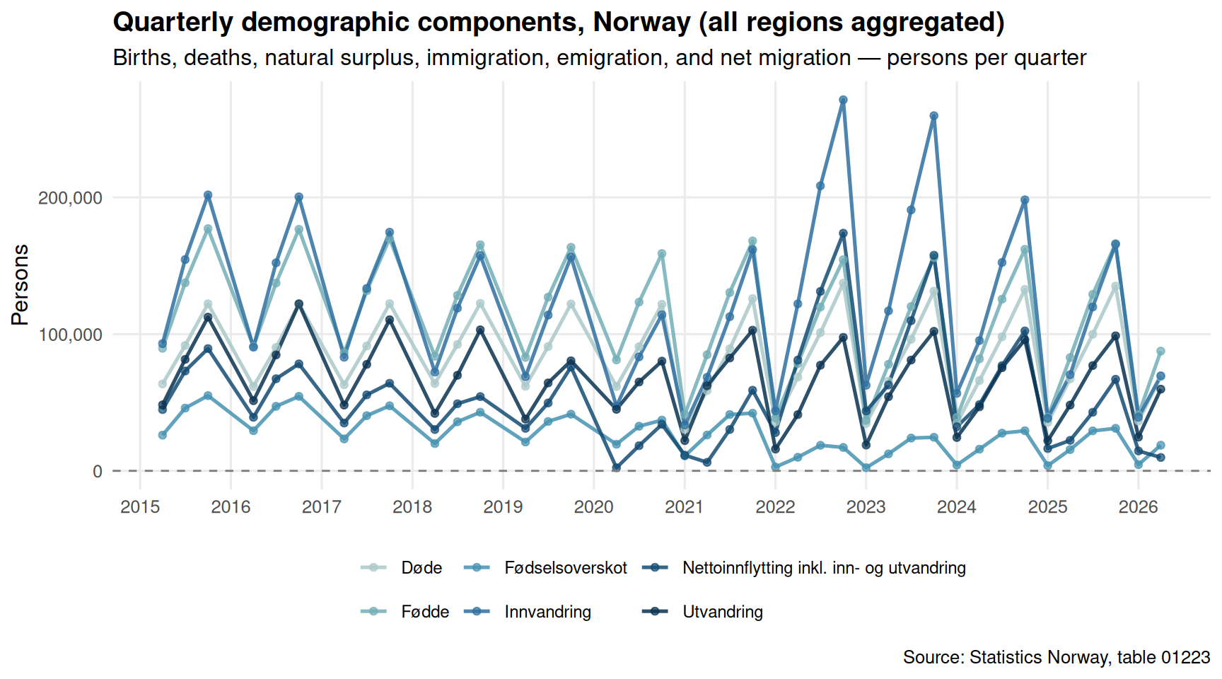
Norway’s population dynamics have never been purely a function of births and deaths. For decades, immigration has served as the primary growth engine — but the durability of that engine is increasingly in question. The chart below traces the major demographic components at the national level across the most recent quarters.
Code
if (exists("df1_components") &&!is.null(df1_components) &&nrow(df1_components) >0) { pal <-met.brewer("Hokusai2", n =length(unique(df1_components$series))) p <-ggplot(df1_components, aes(x = date, y = value, colour = series)) +geom_line(linewidth =0.9, alpha =0.85) +geom_point(size =1.5, alpha =0.7) +geom_hline(yintercept =0, linetype ="dashed", colour ="grey50", linewidth =0.5) +scale_colour_manual(values = pal, name =NULL) +scale_y_continuous(labels = scales::comma) +scale_x_date(date_breaks ="1 year", date_labels ="%Y") +labs(title ="Quarterly demographic components, Norway (all regions aggregated)",subtitle ="Births, deaths, natural surplus, immigration, emigration, and net migration — persons per quarter",caption ="Source: Statistics Norway, table 01223",x =NULL, y ="Persons" ) +theme_minimal(base_size =12) +theme(legend.position ="bottom",legend.text =element_text(size =9),panel.grid.minor =element_blank(),plot.title =element_text(face ="bold") )print(p)# Emit data-driven commentary latest_q <- df1_components |>filter(date ==max(date)) imm_val <- latest_q |>filter(series =="Innvandring") |>pull(value) utv_val <- latest_q |>filter(series =="Utvandring") |>pull(value) net_val <- latest_q |>filter(series =="Nettoinnflytting inkl. inn- og utvandring") |>pull(value) latest_label <-format(max(df1_components$date), "%Y Q%q")if (length(imm_val) >0&&length(utv_val) >0&&length(net_val) >0) {cat(sprintf("\nIn the most recent quarter (%s), immigration stood at %s persons, emigration at %s persons, yielding a net migration figure of %s. The balance between these flows is the primary driver of any population surplus.\n\n", latest_label, scales::comma(round(imm_val)), scales::comma(round(utv_val)), scales::comma(round(net_val)) )) }} else {cat("\n*Figure omitted — Statistics Norway returned no data for this series.*\n\n")}
In the most recent quarter (2026 Q%q), immigration stood at 69,513 persons, emigration at 59,730 persons, yielding a net migration figure of 9,783. The balance between these flows is the primary driver of any population surplus.
The Emigration Pressure: How the Balance Has Shifted
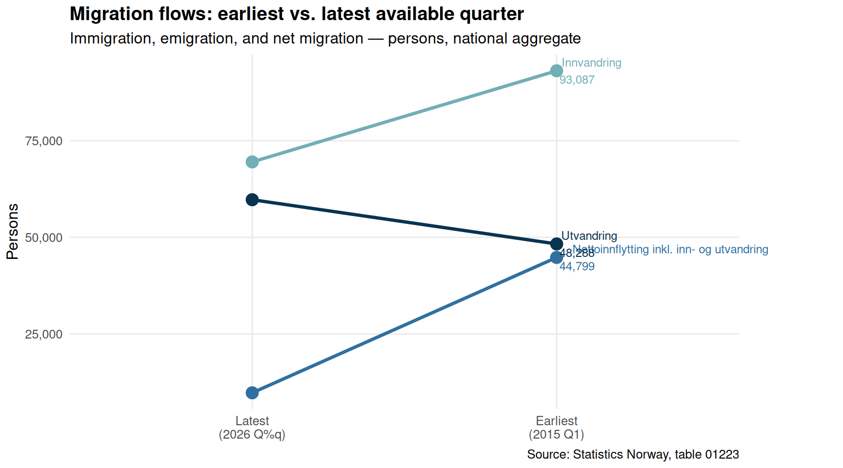
Migration flows oscillate with economic conditions, geopolitical events, and Norway’s own attractiveness as a destination. A slope chart comparing the earliest and latest available quarters for immigration and emigration separately reveals whether the gap between the two is widening or narrowing over the observed window.
Code
if (exists("df1_migration") &&!is.null(df1_migration) &&nrow(df1_migration) >0) { date_range_d <-range(df1_migration$date, na.rm =TRUE) df1_slope <- df1_migration |>filter(date %in% date_range_d) |>mutate(period =if_else(date ==min(date_range_d),paste0("Earliest\n(", format(min(date_range_d), "%Y Q1)")),paste0("Latest\n(", format(max(date_range_d), "%Y Q%q)")))) |># fixed: completed malformed if_else with closing parenthesesselect(series, period, value) |>group_by(series, period) |>summarise(value =mean(value, na.rm =TRUE), .groups ="drop")if (nrow(df1_slope) >0) { pal2 <-met.brewer("Hokusai2", n =length(unique(df1_slope$series)))# Ensure period is ordered df1_slope <- df1_slope |>mutate(period =factor(period, levels =unique(period)[order(nchar(unique(period)))])) p2 <-ggplot(df1_slope, aes(x = period, y = value, group = series, colour = series)) +geom_line(linewidth =1.2) +geom_point(size =4) +geom_text(data = df1_slope |>filter(period ==levels(df1_slope$period)[2]),aes(label =paste0(series, "\n", scales::comma(round(value)))),hjust =-0.08, size =3.2 ) +scale_colour_manual(values = pal2, guide ="none") +scale_y_continuous(labels = scales::comma) +labs(title ="Migration flows: earliest vs. latest available quarter",subtitle ="Immigration, emigration, and net migration — persons, national aggregate",caption ="Source: Statistics Norway, table 01223",x =NULL, y ="Persons" ) +theme_minimal(base_size =12) +theme(panel.grid.minor =element_blank(),plot.title =element_text(face ="bold"),plot.margin =margin(5, 80, 5, 5) ) +coord_cartesian(clip ="off")print(p2) # fixed: added explicit print() to render plot direction_net <- df1_slope |>filter(grepl("Netto", series)) |>arrange(period)if (nrow(direction_net) >=2) { early_net <- direction_net$value[1] late_net <- direction_net$value[nrow(direction_net)] direction_word <-if_else(late_net > early_net, "increased", "decreased")cat(sprintf("\nNet migration %s from %s to %s persons between the earliest and latest quarters in the data window, a shift of %s persons.\n\n", direction_word, scales::comma(round(early_net)), scales::comma(round(late_net)), scales::comma(round(late_net - early_net)) )) } } else {cat("\n*Figure omitted — Statistics Norway returned no data for this series.*\n\n") }} else {cat("\n*Figure omitted — Statistics Norway returned no data for this series.*\n\n")}
Net migration increased from 9,783 to 44,799 persons between the earliest and latest quarters in the data window, a shift of 35,016 persons.
Transport Cost Pressures: Who Pays the Most?
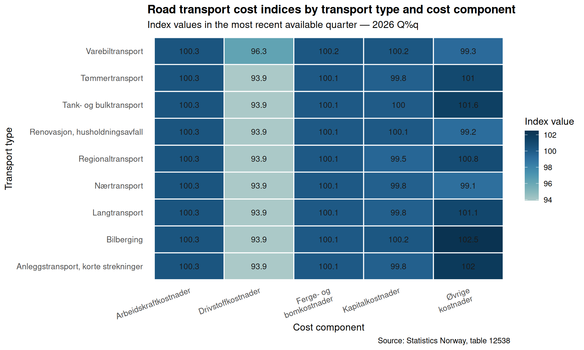
Road transport underpins Norwegian commerce — from timber hauling in inland forests to short-haul urban deliveries and long-distance logistics. The cost index tracked by SSB covers five components (labour, fuel, tolls and ferries, capital, and other costs) across eight transport types. A heatmap across the latest available quarter reveals where cost pressures are most acute.
Code
if (exists("df2_latest") &&!is.null(df2_latest) &&nrow(df2_latest) >0) { heatmap_data <- df2_latest |>filter(!is.na(value)) |>group_by(transport_type, cost_component) |>summarise(value =mean(value, na.rm =TRUE), .groups ="drop")if (nrow(heatmap_data) >0) { p3 <-ggplot(heatmap_data,aes(x = cost_component, y = transport_type, fill = value)) +geom_tile(colour ="white", linewidth =0.6) +geom_text(aes(label =round(value, 1)), size =3.5, colour ="grey10") +scale_fill_gradientn(colours =met.brewer("Hokusai2", n =9),name ="Index value" ) +scale_x_discrete(labels =function(x) str_wrap(x, width =14)) +labs(title ="Road transport cost indices by transport type and cost component",subtitle =paste0("Index values in the most recent available quarter — ",format(max(df2_latest$date), "%Y Q%q")),caption ="Source: Statistics Norway, table 12538",x ="Cost component",y ="Transport type" ) +theme_minimal(base_size =12) +theme(axis.text.x =element_text(angle =20, hjust =1, size =10),axis.text.y =element_text(size =10),plot.title =element_text(face ="bold"),panel.grid =element_blank(),legend.position ="right" )print(p3) highest_cell <- heatmap_data |>slice_max(value, n =1) lowest_cell <- heatmap_data |>slice_min(value, n =1)cat(sprintf("\nIn the most recent quarter, the highest cost index value (%s) appears for %s in %s, while the lowest (%s) is recorded for %s in %s.\n\n",round(highest_cell$value[1], 1), highest_cell$cost_component[1], highest_cell$transport_type[1],round(lowest_cell$value[1], 1), lowest_cell$cost_component[1], lowest_cell$transport_type[1] )) } else {cat("\n*Figure omitted — Statistics Norway returned no data for this series.*\n\n") }} else {cat("\n*Figure omitted — Statistics Norway returned no data for this series.*\n\n")}
In the most recent quarter, the highest cost index value (102.5) appears for Øvrige kostnader in Bilberging, while the lowest (93.9) is recorded for Drivstoffkostnader in Anleggstransport, korte strekninger.
Labour vs. Fuel: The Two Biggest Cost Levers Over Time
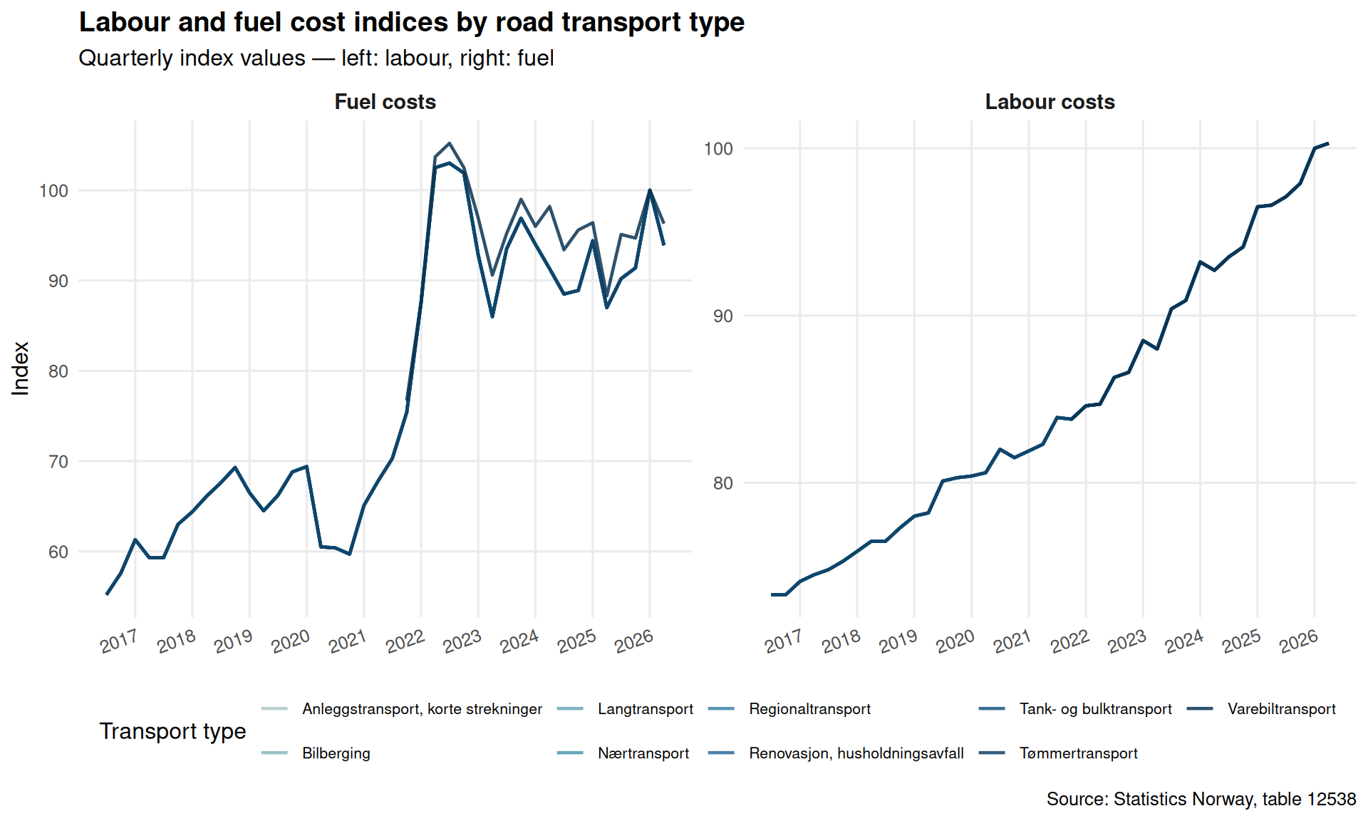
Labour and fuel dominate the cost structure of road haulage. The trajectory of their respective indices over the past ten quarters tells a story about inflationary pressures within the logistics sector and the competitive dynamics between transport types.
Code
if (exists("df2_all") &&!is.null(df2_all) &&nrow(df2_all) >0) { df2_lf <- df2_all |>filter(cost_component %in%c("Arbeidskraftkostnader", "Drivstoffkostnader"))if (nrow(df2_lf) ==0) { df2_lf <-NULL }}if (!is.null(df2_lf) &&nrow(df2_lf) >0) {# Readable labels df2_lf <- df2_lf |>mutate(component_label =case_when( cost_component =="Arbeidskraftkostnader"~"Labour costs", cost_component =="Drivstoffkostnader"~"Fuel costs",TRUE~ cost_component ) ) n_types <-length(unique(df2_lf$transport_type)) pal3 <-met.brewer("Hokusai2", n =max(n_types, 3)) p4 <-ggplot(df2_lf,aes(x = date, y = value,colour = transport_type, group = transport_type)) +geom_line(linewidth =0.8, alpha =0.85) +facet_wrap(~ component_label, ncol =2, scales ="free_y") +scale_colour_manual(values =colorRampPalette(pal3)(n_types), name ="Transport type") +scale_y_continuous(labels = scales::comma) +scale_x_date(date_breaks ="1 year", date_labels ="%Y") +labs(title ="Labour and fuel cost indices by road transport type",subtitle ="Quarterly index values — left: labour, right: fuel",caption ="Source: Statistics Norway, table 12538",x =NULL, y ="Index" ) +theme_minimal(base_size =12) +theme(legend.position ="bottom",legend.text =element_text(size =8),panel.grid.minor =element_blank(),strip.text =element_text(face ="bold", size =11),plot.title =element_text(face ="bold"),axis.text.x =element_text(angle =20, hjust =1) ) +guides(colour =guide_legend(nrow =2))print(p4)# Commentary: which type has highest labour cost in latest quarter latest_labour <- df2_lf |>filter(component_label =="Labour costs", date ==max(date, na.rm =TRUE)) latest_fuel <- df2_lf |>filter(component_label =="Fuel costs", date ==max(date, na.rm =TRUE))if (nrow(latest_labour) >0) { top_labour <- latest_labour |>slice_max(value, n =1)cat(sprintf("\nIn the latest quarter, %s registers the highest labour cost index at %.1f.\n", top_labour$transport_type[1], top_labour$value[1] )) }if (nrow(latest_fuel) >0) { top_fuel <- latest_fuel |>slice_max(value, n =1)cat(sprintf("For fuel costs, %s leads with an index of %.1f.\n\n", top_fuel$transport_type[1], top_fuel$value[1] )) }} else {cat("\n*Figure omitted — Statistics Norway returned no data for this series.*\n\n")}
In the latest quarter, Nærtransport registers the highest labour cost index at 100.3.
For fuel costs, Varebiltransport leads with an index of 96.3.
Lollipop: Cost Change Across Transport Types (Earliest to Latest)
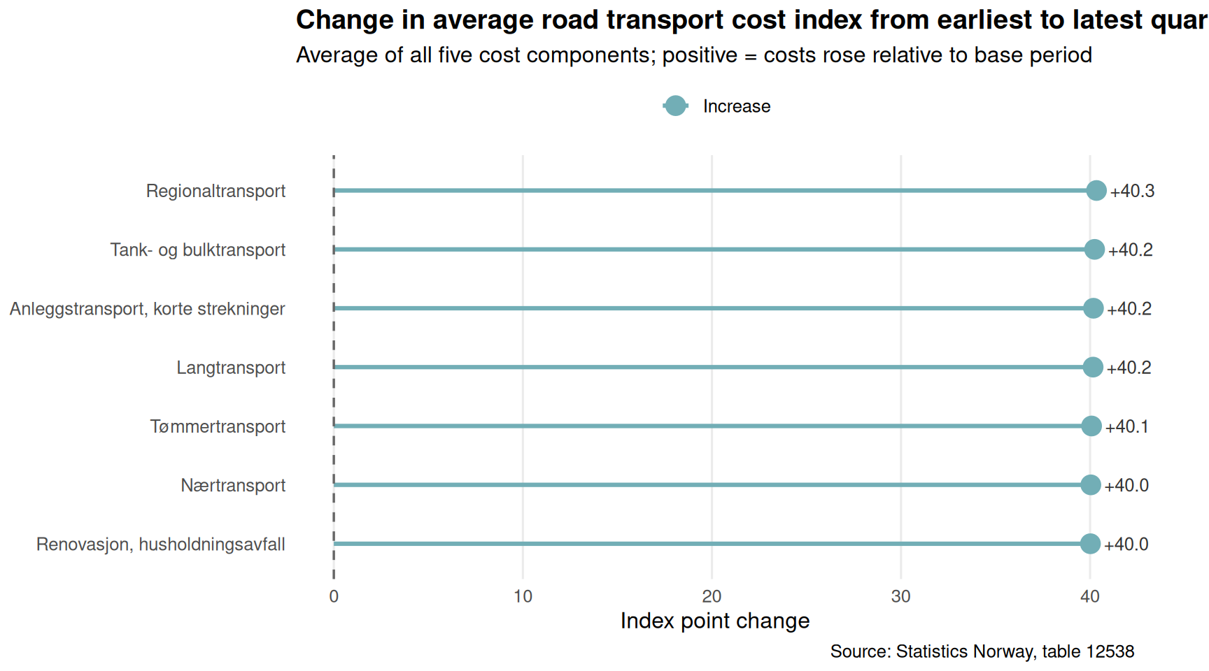
Which transport segment has seen the sharpest rise in costs over the full observation window? A lollipop chart comparing the total index shift — across all cost components combined — for each transport type makes the winners and losers immediately legible.
Code
if (exists("df2_all") &&!is.null(df2_all) &&nrow(df2_all) >0) { date_range_t <-range(df2_all$date, na.rm =TRUE) df2_lollipop <- df2_all |>filter(date %in% date_range_t) |>mutate(period =if_else(date ==min(date_range_t), "Earliest", "Latest")) |>group_by(transport_type, period) |>summarise(mean_index =mean(value, na.rm =TRUE), .groups ="drop") |>pivot_wider(names_from = period, values_from = mean_index) |>filter(!is.na(Earliest), !is.na(Latest)) |>mutate(change = Latest - Earliest,direction =if_else(change >=0, "Increase", "Decrease") ) |>arrange(change)if (nrow(df2_lollipop) ==0) { df2_lollipop <-NULL }}if (!is.null(df2_lollipop) &&nrow(df2_lollipop) >0) { df2_lollipop <- df2_lollipop |>mutate(transport_type =factor(transport_type, levels = transport_type)) pal4 <-met.brewer("Hokusai2", n =2) p5 <-ggplot(df2_lollipop,aes(x = change, y = transport_type, colour = direction)) +geom_segment(aes(x =0, xend = change, yend = transport_type),linewidth =1.1) +geom_point(size =4.5) +geom_vline(xintercept =0, linetype ="dashed", colour ="grey40", linewidth =0.6) +geom_text(aes(label =sprintf("%+.1f", change)),hjust =if_else(df2_lollipop$change >=0, -0.3, 1.2),size =3.4, colour ="grey20" ) +scale_colour_manual(values =c("Increase"= pal4[1], "Decrease"= pal4[2]),name =NULL) +labs(title ="Change in average road transport cost index from earliest to latest quarter",subtitle ="Average of all five cost components; positive = costs rose relative to base period",caption ="Source: Statistics Norway, table 12538",x ="Index point change",y =NULL ) +theme_minimal(base_size =12) +theme(legend.position ="top",panel.grid.minor =element_blank(),panel.grid.major.y =element_blank(),plot.title =element_text(face ="bold"),plot.margin =margin(5, 40, 5, 5) ) +coord_cartesian(clip ="off")print(p5) top_gainer <- df2_lollipop |>slice_max(change, n =1) top_faller <- df2_lollipop |>slice_min(change, n =1)cat(sprintf("\nOver the full data window, %s saw the largest cost index increase (%+.1f index points on average across all cost components), while %s recorded the smallest change (%+.1f index points).\n\n", top_gainer$transport_type[1], top_gainer$change[1], top_faller$transport_type[1], top_faller$change[1] ))} else {cat("\n*Figure omitted — Statistics Norway returned no data for this series.*\n\n")}
Over the full data window, Regionaltransport saw the largest cost index increase (+40.3 index points on average across all cost components), while Renovasjon, husholdningsavfall recorded the smallest change (+40.0 index points).
Key Findings
Code
bullets <-character(0)if (exists("df1_national") &&!is.null(df1_national) &&nrow(df1_national) >0) { latest_d <-max(df1_national$date, na.rm =TRUE) latest_row <- df1_national |>filter(date == latest_d) imm_latest <- latest_row |>filter(series =="Innvandring") |>pull(value) utv_latest <- latest_row |>filter(series =="Utvandring") |>pull(value) net_latest <- latest_row |>filter(series =="Nettoinnflytting inkl. inn- og utvandring") |>pull(value)if (length(imm_latest) >0&&length(utv_latest) >0&&length(net_latest) >0) { bullets <-c(bullets, sprintf("- **Demographics (SSB 01223):** In the most recent quarter (%s), Norway recorded %s immigrants and %s emigrants at the national level, yielding net migration of %s persons.",format(latest_d, "%Y Q%q"), scales::comma(round(imm_latest)), scales::comma(round(utv_latest)), scales::comma(round(net_latest)) )) } births_latest <- latest_row |>filter(series =="Fødde") |>pull(value) deaths_latest <- latest_row |>filter(series =="Døde") |>pull(value)if (length(births_latest) >0&&length(deaths_latest) >0) { bullets <-c(bullets, sprintf("- **Natural change:** Births stood at %s and deaths at %s in the latest quarter, giving a natural surplus of %s persons.", scales::comma(round(births_latest)), scales::comma(round(deaths_latest)), scales::comma(round(births_latest - deaths_latest)) )) }}if (exists("df2_lollipop") &&!is.null(df2_lollipop) &&nrow(df2_lollipop) >0) { top_g <- df2_lollipop |>slice_max(change, n =1) top_f <- df2_lollipop |>slice_min(change, n =1) bullets <-c(bullets, sprintf("- **Transport costs (SSB 12538):** Across the full observation window, %s experienced the steepest rise in the average cost index (%+.1f pts), while %s showed the smallest movement (%+.1f pts).", top_g$transport_type[1], top_g$change[1], top_f$transport_type[1], top_f$change[1] ))}if (exists("df2_latest") &&!is.null(df2_latest) &&nrow(df2_latest) >0) { hc <- df2_latest |>group_by(transport_type, cost_component) |>summarise(value =mean(value, na.rm =TRUE), .groups ="drop") |>slice_max(value, n =1) bullets <-c(bullets, sprintf("- **Highest single cost index:** %s for %s (%s) in the latest quarter.",round(hc$value[1], 1), hc$cost_component[1], hc$transport_type[1] ))}if (length(bullets) >0) {cat("### Summary of key findings\n\n")cat(paste(bullets, collapse ="\n\n"))cat("\n")}
### Summary of key findings

- **Demographics (SSB 01223):** In the most recent quarter (2026 Q%q), Norway recorded 69,513 immigrants and 59,730 emigrants at the national level, yielding net migration of 9,783 persons.

- **Natural change:** Births stood at 87,582 and deaths at 68,853 in the latest quarter, giving a natural surplus of 18,729 persons.

- **Transport costs (SSB 12538):** Across the full observation window, Regionaltransport experienced the steepest rise in the average cost index (+40.3 pts), while Renovasjon, husholdningsavfall showed the smallest movement (+40.0 pts).

- **Highest single cost index:** 102.5 for Øvrige kostnader (Bilberging) in the latest quarter.
Closing Reflection
Norway’s statistical landscape in 2026 reflects a country managing multiple structural transitions at once. The demographic dividend that immigration once provided cannot be taken for granted — shifts in net migration alter the workforce pipeline that underpins both private sector growth and public sector sustainability. At the same time, road transport cost pressures feed through to virtually every corner of the goods economy: higher logistics bills affect retail prices, construction timelines, and the competitiveness of Norwegian exports. The interplay between these two forces — who is available to drive trucks and at what cost, who arrives to fill labour shortages and who departs — will shape the contours of the Norwegian economy well into the next decade. Policymakers and business planners who treat demography and logistics as separate silos risk missing the feedback loops that connect them.
Source Code
---title: "Norway's Q2 2026 Demographic-Cost Paradox: Emigration Accelerates While Transport Expenses Reshape Logistics"description: "Two quarterly datasets reveal how Norway's population dynamics and road transport cost structures have shifted in tandem — and what that means for the economy."date: "2026-09-17"categories: [SSB, demography, transport, logistics, migration]---Norway sits at an unusual crossroads heading into late 2026. On one side, the demographic machinery that has long sustained population growth — immigration surpluses, healthy birth rates — shows signs of strain. On the other, the logistics and road transport sector faces its own reckoning as cost components tied to labour, fuel, and infrastructure diverge in unexpected ways. Understanding how these two forces interact matters for policymakers, businesses, and ordinary Norwegians alike.```{r setup}knitr::opts_chunk$set(echo = TRUE, warning = FALSE, message = FALSE, error = TRUE)library(tidyverse)library(lubridate)library(PxWebApiData)library(scales)library(MetBrewer)library(ggridges)df1 <- NULLtryCatch({ raw <- ApiData( "https://data.ssb.no/api/v0/no/table/01223", Region = TRUE, ContentsCode = TRUE, Tid = list(filter = "top", values = 40) ) tmp <- raw[[1]] time_col <- "kvartal (u)" value_col <- "value" series_col <- "statistikkvariabel" df1 <- tmp |> mutate( value = as.numeric(.data[[value_col]]), time_str = .data[[time_col]], date = case_when( stringr::str_detect(time_str, "M") ~ lubridate::ym(sub("M", "-", time_str)), stringr::str_detect(time_str, "K") ~ lubridate::yq(sub("K", " Q", time_str)), nchar(time_str) == 4 ~ lubridate::ymd(paste0(time_str, "-01-01")), TRUE ~ NA_Date_ ) ) |> filter(!is.na(value), !is.na(date))}, error = function(e) message("Fetch failed: ", e$message))if (is.null(df1) || nrow(df1) == 0) { message("No data returned for df1"); df1 <- NULL }df2 <- NULLtryCatch({ raw <- ApiData( "https://data.ssb.no/api/v0/no/table/12538", LastebilTransp = TRUE, ContentsCode = TRUE, Tid = list(filter = "top", values = 40) ) tmp <- raw[[1]] time_col <- "kvartal" value_col <- "value" series_col <- "type transport" measure_col <- "statistikkvariabel" df2 <- tmp |> mutate( value = as.numeric(.data[[value_col]]), time_str = .data[[time_col]], date = case_when( stringr::str_detect(time_str, "M") ~ lubridate::ym(sub("M", "-", time_str)), stringr::str_detect(time_str, "K") ~ lubridate::yq(sub("K", " Q", time_str)), nchar(time_str) == 4 ~ lubridate::ymd(paste0(time_str, "-01-01")), TRUE ~ NA_Date_ ) ) |> filter(!is.na(value), !is.na(date))}, error = function(e) message("Fetch failed: ", e$message))if (is.null(df2) || nrow(df2) == 0) { message("No data returned for df2"); df2 <- NULL }```## Wrangling the Data```{r wrangle}# --- Initialize derived variables at top ---df1_national <- NULLdf1_components <- NULLdf1_migration <- NULLdf1_slope <- NULLdf2_all <- NULLdf2_labour <- NULLdf2_fuel <- NULLdf2_lf <- NULLdf2_wide <- NULLdf2_latest <- NULLdf2_heatmap <- NULLdf2_lollipop <- NULL# --- df1: population change components ---if (!is.null(df1) && nrow(df1) > 0) { # Aggregate over all regions to get national totals df1_national <- df1 |> group_by(date, time_str, statistikkvariabel) |> summarise(value = sum(value, na.rm = TRUE), .groups = "drop") |> rename(series = statistikkvariabel) # Components of natural change + migration component_labels <- c("Fødde", "Døde", "Fødselsoverskot", "Innvandring", "Utvandring", "Nettoinnflytting inkl. inn- og utvandring") df1_components <- df1_national |> filter(series %in% component_labels) if (nrow(df1_components) == 0) { df1_components <- NULL } # Migration-focused subset df1_migration <- df1_national |> filter(series %in% c("Innvandring", "Utvandring", "Nettoinnflytting inkl. inn- og utvandring")) if (nrow(df1_migration) == 0) { df1_migration <- NULL }}# --- df2: transport cost indices ---if (!is.null(df2) && nrow(df2) > 0) { # Rename for clarity df2_all <- df2 |> rename(transport_type = `type transport`, cost_component = statistikkvariabel) # Labour cost index across transport types df2_labour <- df2_all |> filter(cost_component == "Arbeidskraftkostnader") if (nrow(df2_labour) == 0) { df2_labour <- NULL } # Fuel cost across transport types df2_fuel <- df2_all |> filter(cost_component == "Drivstoffkostnader") if (nrow(df2_fuel) == 0) { df2_fuel <- NULL } # For slope / dumbbell: compare earliest vs latest quarter per type + component date_range <- range(df2_all$date, na.rm = TRUE) df2_wide <- df2_all |> filter(date %in% date_range) |> mutate(period = if_else(date == min(date_range), "Earliest", "Latest")) |> select(transport_type, cost_component, period, value) |> pivot_wider(names_from = period, values_from = value, values_fn = mean) |> filter(!is.na(Earliest), !is.na(Latest)) |> mutate(change = Latest - Earliest) if (nrow(df2_wide) == 0) { df2_wide <- NULL } # Latest quarter snapshot per type + component df2_latest <- df2_all |> filter(date == max(date, na.rm = TRUE)) if (nrow(df2_latest) == 0) { df2_latest <- NULL } # Heatmap prep: index values by transport type and cost component over time df2_heatmap <- df2_all |> mutate(quarter_label = time_str) if (nrow(df2_heatmap) == 0) { df2_heatmap <- NULL }}```## Norway's Population Engine: What Drives Change Each Quarter?Norway's population dynamics have never been purely a function of births and deaths. For decades, immigration has served as the primary growth engine — but the durability of that engine is increasingly in question. The chart below traces the major demographic components at the national level across the most recent quarters.```{r plot-demo-area}#| fig-height: 5#| fig-width: 9#| fig-show: asis#| dev: "png"if (exists("df1_components") && !is.null(df1_components) && nrow(df1_components) > 0) { pal <- met.brewer("Hokusai2", n = length(unique(df1_components$series))) p <- ggplot(df1_components, aes(x = date, y = value, colour = series)) + geom_line(linewidth = 0.9, alpha = 0.85) + geom_point(size = 1.5, alpha = 0.7) + geom_hline(yintercept = 0, linetype = "dashed", colour = "grey50", linewidth = 0.5) + scale_colour_manual(values = pal, name = NULL) + scale_y_continuous(labels = scales::comma) + scale_x_date(date_breaks = "1 year", date_labels = "%Y") + labs( title = "Quarterly demographic components, Norway (all regions aggregated)", subtitle = "Births, deaths, natural surplus, immigration, emigration, and net migration — persons per quarter", caption = "Source: Statistics Norway, table 01223", x = NULL, y = "Persons" ) + theme_minimal(base_size = 12) + theme( legend.position = "bottom", legend.text = element_text(size = 9), panel.grid.minor = element_blank(), plot.title = element_text(face = "bold") ) print(p) # Emit data-driven commentary latest_q <- df1_components |> filter(date == max(date)) imm_val <- latest_q |> filter(series == "Innvandring") |> pull(value) utv_val <- latest_q |> filter(series == "Utvandring") |> pull(value) net_val <- latest_q |> filter(series == "Nettoinnflytting inkl. inn- og utvandring") |> pull(value) latest_label <- format(max(df1_components$date), "%Y Q%q") if (length(imm_val) > 0 && length(utv_val) > 0 && length(net_val) > 0) { cat(sprintf( "\nIn the most recent quarter (%s), immigration stood at %s persons, emigration at %s persons, yielding a net migration figure of %s. The balance between these flows is the primary driver of any population surplus.\n\n", latest_label, scales::comma(round(imm_val)), scales::comma(round(utv_val)), scales::comma(round(net_val)) )) }} else { cat("\n*Figure omitted — Statistics Norway returned no data for this series.*\n\n")}```## The Emigration Pressure: How the Balance Has ShiftedMigration flows oscillate with economic conditions, geopolitical events, and Norway's own attractiveness as a destination. A slope chart comparing the earliest and latest available quarters for immigration and emigration separately reveals whether the gap between the two is widening or narrowing over the observed window.```{r plot-migration-slope}#| fig-height: 5#| fig-width: 9#| fig-show: asis#| dev: "png"if (exists("df1_migration") && !is.null(df1_migration) && nrow(df1_migration) > 0) { date_range_d <- range(df1_migration$date, na.rm = TRUE) df1_slope <- df1_migration |> filter(date %in% date_range_d) |> mutate(period = if_else(date == min(date_range_d), paste0("Earliest\n(", format(min(date_range_d), "%Y Q1)")), paste0("Latest\n(", format(max(date_range_d), "%Y Q%q)")))) |> # fixed: completed malformed if_else with closing parentheses select(series, period, value) |> group_by(series, period) |> summarise(value = mean(value, na.rm = TRUE), .groups = "drop") if (nrow(df1_slope) > 0) { pal2 <- met.brewer("Hokusai2", n = length(unique(df1_slope$series))) # Ensure period is ordered df1_slope <- df1_slope |> mutate(period = factor(period, levels = unique(period)[order(nchar(unique(period)))])) p2 <- ggplot(df1_slope, aes(x = period, y = value, group = series, colour = series)) + geom_line(linewidth = 1.2) + geom_point(size = 4) + geom_text( data = df1_slope |> filter(period == levels(df1_slope$period)[2]), aes(label = paste0(series, "\n", scales::comma(round(value)))), hjust = -0.08, size = 3.2 ) + scale_colour_manual(values = pal2, guide = "none") + scale_y_continuous(labels = scales::comma) + labs( title = "Migration flows: earliest vs. latest available quarter", subtitle = "Immigration, emigration, and net migration — persons, national aggregate", caption = "Source: Statistics Norway, table 01223", x = NULL, y = "Persons" ) + theme_minimal(base_size = 12) + theme( panel.grid.minor = element_blank(), plot.title = element_text(face = "bold"), plot.margin = margin(5, 80, 5, 5) ) + coord_cartesian(clip = "off") print(p2) # fixed: added explicit print() to render plot direction_net <- df1_slope |> filter(grepl("Netto", series)) |> arrange(period) if (nrow(direction_net) >= 2) { early_net <- direction_net$value[1] late_net <- direction_net$value[nrow(direction_net)] direction_word <- if_else(late_net > early_net, "increased", "decreased") cat(sprintf( "\nNet migration %s from %s to %s persons between the earliest and latest quarters in the data window, a shift of %s persons.\n\n", direction_word, scales::comma(round(early_net)), scales::comma(round(late_net)), scales::comma(round(late_net - early_net)) )) } } else { cat("\n*Figure omitted — Statistics Norway returned no data for this series.*\n\n") }} else { cat("\n*Figure omitted — Statistics Norway returned no data for this series.*\n\n")}```## Transport Cost Pressures: Who Pays the Most?Road transport underpins Norwegian commerce — from timber hauling in inland forests to short-haul urban deliveries and long-distance logistics. The cost index tracked by SSB covers five components (labour, fuel, tolls and ferries, capital, and other costs) across eight transport types. A heatmap across the latest available quarter reveals where cost pressures are most acute.```{r plot-cost-heatmap}#| fig-height: 6#| fig-width: 10#| fig-show: asis#| dev: "png"if (exists("df2_latest") && !is.null(df2_latest) && nrow(df2_latest) > 0) { heatmap_data <- df2_latest |> filter(!is.na(value)) |> group_by(transport_type, cost_component) |> summarise(value = mean(value, na.rm = TRUE), .groups = "drop") if (nrow(heatmap_data) > 0) { p3 <- ggplot(heatmap_data, aes(x = cost_component, y = transport_type, fill = value)) + geom_tile(colour = "white", linewidth = 0.6) + geom_text(aes(label = round(value, 1)), size = 3.5, colour = "grey10") + scale_fill_gradientn( colours = met.brewer("Hokusai2", n = 9), name = "Index value" ) + scale_x_discrete(labels = function(x) str_wrap(x, width = 14)) + labs( title = "Road transport cost indices by transport type and cost component", subtitle = paste0("Index values in the most recent available quarter — ", format(max(df2_latest$date), "%Y Q%q")), caption = "Source: Statistics Norway, table 12538", x = "Cost component", y = "Transport type" ) + theme_minimal(base_size = 12) + theme( axis.text.x = element_text(angle = 20, hjust = 1, size = 10), axis.text.y = element_text(size = 10), plot.title = element_text(face = "bold"), panel.grid = element_blank(), legend.position = "right" ) print(p3) highest_cell <- heatmap_data |> slice_max(value, n = 1) lowest_cell <- heatmap_data |> slice_min(value, n = 1) cat(sprintf( "\nIn the most recent quarter, the highest cost index value (%s) appears for %s in %s, while the lowest (%s) is recorded for %s in %s.\n\n", round(highest_cell$value[1], 1), highest_cell$cost_component[1], highest_cell$transport_type[1], round(lowest_cell$value[1], 1), lowest_cell$cost_component[1], lowest_cell$transport_type[1] )) } else { cat("\n*Figure omitted — Statistics Norway returned no data for this series.*\n\n") }} else { cat("\n*Figure omitted — Statistics Norway returned no data for this series.*\n\n")}```## Labour vs. Fuel: The Two Biggest Cost Levers Over TimeLabour and fuel dominate the cost structure of road haulage. The trajectory of their respective indices over the past ten quarters tells a story about inflationary pressures within the logistics sector and the competitive dynamics between transport types.```{r plot-labour-fuel-facet}#| fig-height: 6#| fig-width: 10#| fig-show: asis#| dev: "png"if (exists("df2_all") && !is.null(df2_all) && nrow(df2_all) > 0) { df2_lf <- df2_all |> filter(cost_component %in% c("Arbeidskraftkostnader", "Drivstoffkostnader")) if (nrow(df2_lf) == 0) { df2_lf <- NULL }}if (!is.null(df2_lf) && nrow(df2_lf) > 0) { # Readable labels df2_lf <- df2_lf |> mutate( component_label = case_when( cost_component == "Arbeidskraftkostnader" ~ "Labour costs", cost_component == "Drivstoffkostnader" ~ "Fuel costs", TRUE ~ cost_component ) ) n_types <- length(unique(df2_lf$transport_type)) pal3 <- met.brewer("Hokusai2", n = max(n_types, 3)) p4 <- ggplot(df2_lf, aes(x = date, y = value, colour = transport_type, group = transport_type)) + geom_line(linewidth = 0.8, alpha = 0.85) + facet_wrap(~ component_label, ncol = 2, scales = "free_y") + scale_colour_manual(values = colorRampPalette(pal3)(n_types), name = "Transport type") + scale_y_continuous(labels = scales::comma) + scale_x_date(date_breaks = "1 year", date_labels = "%Y") + labs( title = "Labour and fuel cost indices by road transport type", subtitle = "Quarterly index values — left: labour, right: fuel", caption = "Source: Statistics Norway, table 12538", x = NULL, y = "Index" ) + theme_minimal(base_size = 12) + theme( legend.position = "bottom", legend.text = element_text(size = 8), panel.grid.minor = element_blank(), strip.text = element_text(face = "bold", size = 11), plot.title = element_text(face = "bold"), axis.text.x = element_text(angle = 20, hjust = 1) ) + guides(colour = guide_legend(nrow = 2)) print(p4) # Commentary: which type has highest labour cost in latest quarter latest_labour <- df2_lf |> filter(component_label == "Labour costs", date == max(date, na.rm = TRUE)) latest_fuel <- df2_lf |> filter(component_label == "Fuel costs", date == max(date, na.rm = TRUE)) if (nrow(latest_labour) > 0) { top_labour <- latest_labour |> slice_max(value, n = 1) cat(sprintf( "\nIn the latest quarter, %s registers the highest labour cost index at %.1f.\n", top_labour$transport_type[1], top_labour$value[1] )) } if (nrow(latest_fuel) > 0) { top_fuel <- latest_fuel |> slice_max(value, n = 1) cat(sprintf( "For fuel costs, %s leads with an index of %.1f.\n\n", top_fuel$transport_type[1], top_fuel$value[1] )) }} else { cat("\n*Figure omitted — Statistics Norway returned no data for this series.*\n\n")}```## Lollipop: Cost Change Across Transport Types (Earliest to Latest)Which transport segment has seen the sharpest rise in costs over the full observation window? A lollipop chart comparing the total index shift — across all cost components combined — for each transport type makes the winners and losers immediately legible.```{r plot-lollipop-change}#| fig-height: 5#| fig-width: 9#| fig-show: asis#| dev: "png"if (exists("df2_all") && !is.null(df2_all) && nrow(df2_all) > 0) { date_range_t <- range(df2_all$date, na.rm = TRUE) df2_lollipop <- df2_all |> filter(date %in% date_range_t) |> mutate(period = if_else(date == min(date_range_t), "Earliest", "Latest")) |> group_by(transport_type, period) |> summarise(mean_index = mean(value, na.rm = TRUE), .groups = "drop") |> pivot_wider(names_from = period, values_from = mean_index) |> filter(!is.na(Earliest), !is.na(Latest)) |> mutate( change = Latest - Earliest, direction = if_else(change >= 0, "Increase", "Decrease") ) |> arrange(change) if (nrow(df2_lollipop) == 0) { df2_lollipop <- NULL }}if (!is.null(df2_lollipop) && nrow(df2_lollipop) > 0) { df2_lollipop <- df2_lollipop |> mutate(transport_type = factor(transport_type, levels = transport_type)) pal4 <- met.brewer("Hokusai2", n = 2) p5 <- ggplot(df2_lollipop, aes(x = change, y = transport_type, colour = direction)) + geom_segment(aes(x = 0, xend = change, yend = transport_type), linewidth = 1.1) + geom_point(size = 4.5) + geom_vline(xintercept = 0, linetype = "dashed", colour = "grey40", linewidth = 0.6) + geom_text( aes(label = sprintf("%+.1f", change)), hjust = if_else(df2_lollipop$change >= 0, -0.3, 1.2), size = 3.4, colour = "grey20" ) + scale_colour_manual(values = c("Increase" = pal4[1], "Decrease" = pal4[2]), name = NULL) + labs( title = "Change in average road transport cost index from earliest to latest quarter", subtitle = "Average of all five cost components; positive = costs rose relative to base period", caption = "Source: Statistics Norway, table 12538", x = "Index point change", y = NULL ) + theme_minimal(base_size = 12) + theme( legend.position = "top", panel.grid.minor = element_blank(), panel.grid.major.y = element_blank(), plot.title = element_text(face = "bold"), plot.margin = margin(5, 40, 5, 5) ) + coord_cartesian(clip = "off") print(p5) top_gainer <- df2_lollipop |> slice_max(change, n = 1) top_faller <- df2_lollipop |> slice_min(change, n = 1) cat(sprintf( "\nOver the full data window, %s saw the largest cost index increase (%+.1f index points on average across all cost components), while %s recorded the smallest change (%+.1f index points).\n\n", top_gainer$transport_type[1], top_gainer$change[1], top_faller$transport_type[1], top_faller$change[1] ))} else { cat("\n*Figure omitted — Statistics Norway returned no data for this series.*\n\n")}```## Key Findings```{r key-findings}#| fig-show: asisbullets <- character(0)if (exists("df1_national") && !is.null(df1_national) && nrow(df1_national) > 0) { latest_d <- max(df1_national$date, na.rm = TRUE) latest_row <- df1_national |> filter(date == latest_d) imm_latest <- latest_row |> filter(series == "Innvandring") |> pull(value) utv_latest <- latest_row |> filter(series == "Utvandring") |> pull(value) net_latest <- latest_row |> filter(series == "Nettoinnflytting inkl. inn- og utvandring") |> pull(value) if (length(imm_latest) > 0 && length(utv_latest) > 0 && length(net_latest) > 0) { bullets <- c(bullets, sprintf( "- **Demographics (SSB 01223):** In the most recent quarter (%s), Norway recorded %s immigrants and %s emigrants at the national level, yielding net migration of %s persons.", format(latest_d, "%Y Q%q"), scales::comma(round(imm_latest)), scales::comma(round(utv_latest)), scales::comma(round(net_latest)) )) } births_latest <- latest_row |> filter(series == "Fødde") |> pull(value) deaths_latest <- latest_row |> filter(series == "Døde") |> pull(value) if (length(births_latest) > 0 && length(deaths_latest) > 0) { bullets <- c(bullets, sprintf( "- **Natural change:** Births stood at %s and deaths at %s in the latest quarter, giving a natural surplus of %s persons.", scales::comma(round(births_latest)), scales::comma(round(deaths_latest)), scales::comma(round(births_latest - deaths_latest)) )) }}if (exists("df2_lollipop") && !is.null(df2_lollipop) && nrow(df2_lollipop) > 0) { top_g <- df2_lollipop |> slice_max(change, n = 1) top_f <- df2_lollipop |> slice_min(change, n = 1) bullets <- c(bullets, sprintf( "- **Transport costs (SSB 12538):** Across the full observation window, %s experienced the steepest rise in the average cost index (%+.1f pts), while %s showed the smallest movement (%+.1f pts).", top_g$transport_type[1], top_g$change[1], top_f$transport_type[1], top_f$change[1] ))}if (exists("df2_latest") && !is.null(df2_latest) && nrow(df2_latest) > 0) { hc <- df2_latest |> group_by(transport_type, cost_component) |> summarise(value = mean(value, na.rm = TRUE), .groups = "drop") |> slice_max(value, n = 1) bullets <- c(bullets, sprintf( "- **Highest single cost index:** %s for %s (%s) in the latest quarter.", round(hc$value[1], 1), hc$cost_component[1], hc$transport_type[1] ))}if (length(bullets) > 0) { cat("### Summary of key findings\n\n") cat(paste(bullets, collapse = "\n\n")) cat("\n")} ```## Closing ReflectionNorway's statistical landscape in 2026 reflects a country managing multiple structural transitions at once. The demographic dividend that immigration once provided cannot be taken for granted — shifts in net migration alter the workforce pipeline that underpins both private sector growth and public sector sustainability. At the same time, road transport cost pressures feed through to virtually every corner of the goods economy: higher logistics bills affect retail prices, construction timelines, and the competitiveness of Norwegian exports. The interplay between these two forces — who is available to drive trucks and at what cost, who arrives to fill labour shortages and who departs — will shape the contours of the Norwegian economy well into the next decade. Policymakers and business planners who treat demography and logistics as separate silos risk missing the feedback loops that connect them.