A data-driven look at how Norway’s housing construction trends, export revenues, and greenhouse gas emissions intersect to reveal the structural tensions in a resource-rich economy.
Published
September 14, 2026
Norway occupies a rare position in the global economy: a petro-state with a green ambition, a construction market buffeted by interest rates, and an export machine whose backbone remains fossil fuels. These three dimensions — housing supply, export composition, and greenhouse gas emissions — rarely appear in the same frame, but they are deeply intertwined. When housing starts fall, it signals stress in the domestic economy. When oil and gas dominate exports, it constrains the energy transition. And when emissions from industry and transport refuse to fall fast enough, the gap between Norway’s climate pledges and its actual trajectory becomes visible in the numbers.
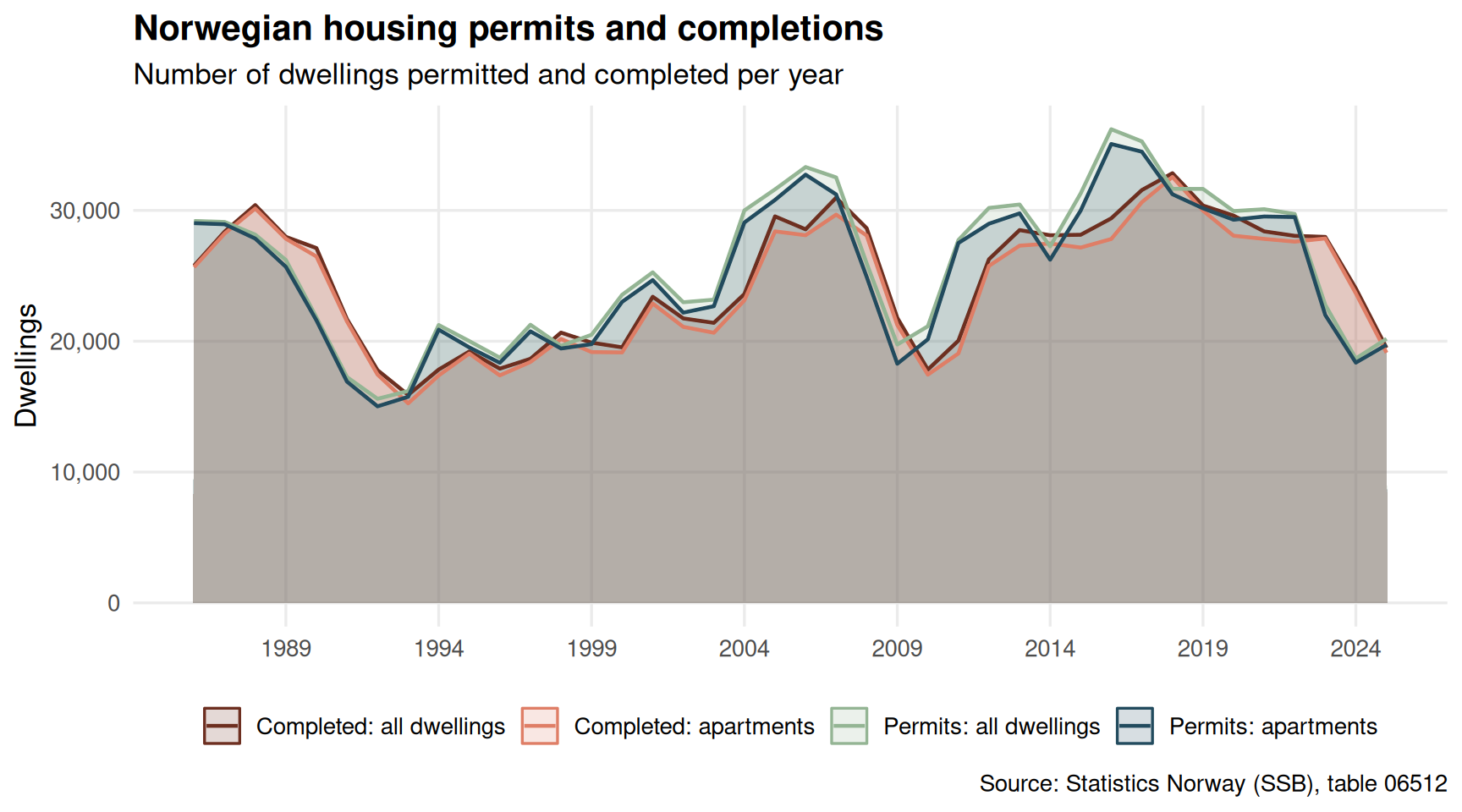
Norway’s housing market has been caught between rising construction costs, elevated interest rates, and persistent demand from population growth. The gap between permits issued and dwellings actually completed is one way to gauge how much of the planned supply ever materialises.
Code
if (exists("df1_housing") &&!is.null(df1_housing) &&nrow(df1_housing) >0) { pal <- MetBrewer::met.brewer("Hokusai1", n =4) label_map <-c("Igangsettingstillatelser boliger"="Permits: all dwellings","Igangsettingstillatelser leiligheter"="Permits: apartments","Fullførte boliger"="Completed: all dwellings","Fullførte leiligheter"="Completed: apartments" ) df1_plot <- df1_housing |>mutate(label = label_map[.data[["statistikkvariabel"]]],label =if_else(is.na(label), .data[["statistikkvariabel"]], label)) p <-ggplot(df1_plot, aes(x = date, y = value, colour = label, fill = label)) +geom_area(alpha =0.18, position ="identity") +geom_line(linewidth =0.8) +scale_colour_manual(values = pal, name =NULL) +scale_fill_manual(values = pal, name =NULL) +scale_y_continuous(labels = scales::comma) +scale_x_date(date_breaks ="5 years", date_labels ="%Y") +labs(title ="Norwegian housing permits and completions",subtitle ="Number of dwellings permitted and completed per year",x =NULL,y ="Dwellings",caption ="Source: Statistics Norway (SSB), table 06512" ) +theme_minimal(base_size =13) +theme(legend.position ="bottom",panel.grid.minor =element_blank(),plot.title =element_text(face ="bold") )print(p) latest_year <-max(df1_housing$year, na.rm =TRUE) latest <- df1_housing |>filter(year == latest_year) permits_tot <- latest |>filter(.data[["statistikkvariabel"]] =="Igangsettingstillatelser boliger") |>pull(value) compl_tot <- latest |>filter(.data[["statistikkvariabel"]] =="Fullførte boliger") |>pull(value)if (length(permits_tot) >0&&length(compl_tot) >0) {cat(sprintf("\nIn %d, SSB recorded %s building permits for all dwellings and %s completions, a gap of %s units.\n\n", latest_year, scales::comma(permits_tot[1]), scales::comma(compl_tot[1]), scales::comma(abs(permits_tot[1] - compl_tot[1])) )) } peak_permits <- df1_housing |>filter(.data[["statistikkvariabel"]] =="Igangsettingstillatelser boliger") |>slice_max(value, n =1)if (nrow(peak_permits) >0) {cat(sprintf("Peak permit activity was recorded in %d with %s permits issued.\n\n", peak_permits$year[1], scales::comma(peak_permits$value[1]) )) }} else {cat("\n*Figure omitted — Statistics Norway returned no data for this series.*\n\n")}
In 2025, SSB recorded 20,184 building permits for all dwellings and 19,498 completions, a gap of 686 units.

Peak permit activity was recorded in 2016 with 36,203 permits issued.
The Lollipop View: Apartment Share of New Construction
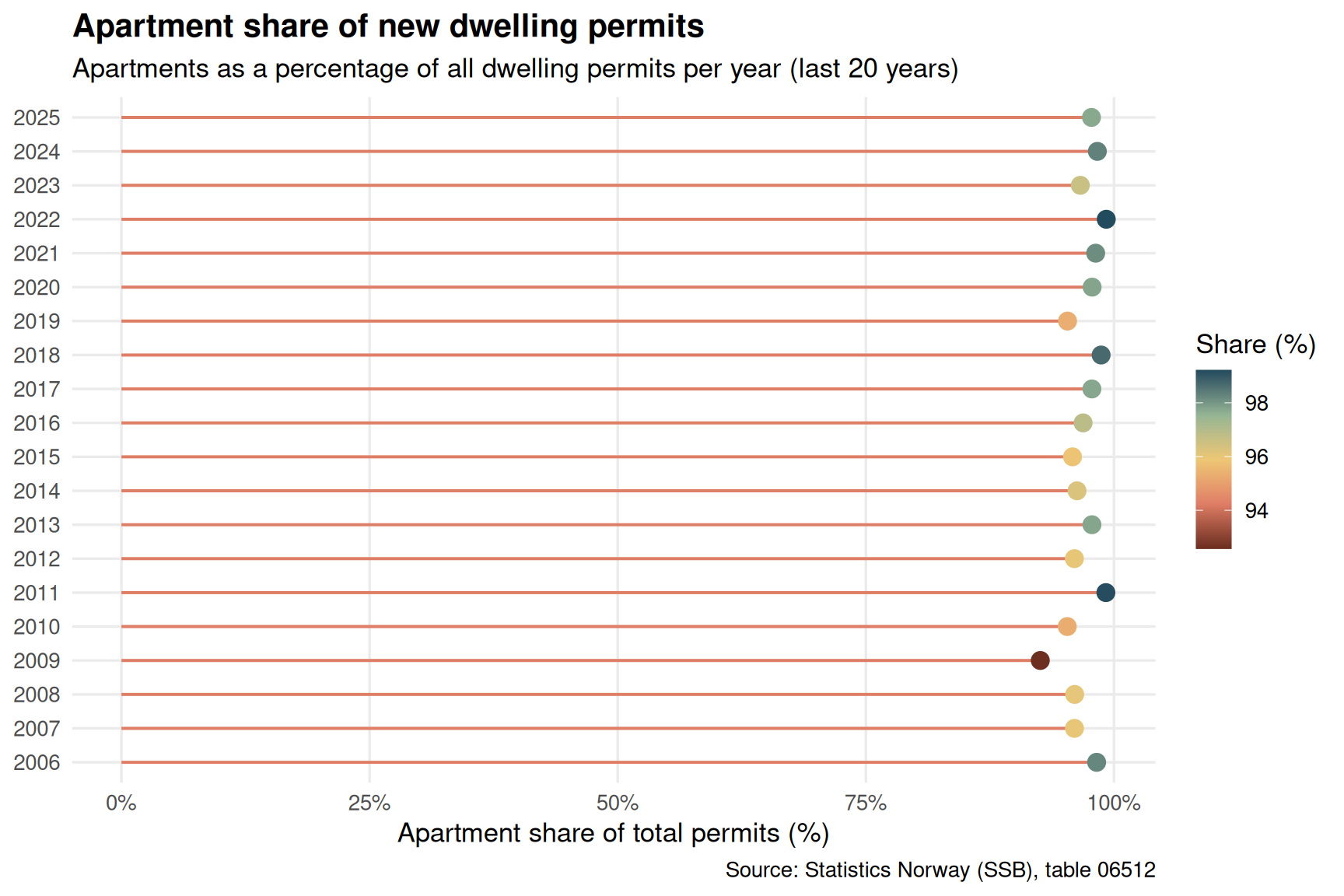
The shift toward apartment-dominated housing supply reflects urbanisation pressures and the changing economics of construction. How large is the apartment share, and has it grown over the period?
Code
if (exists("df1_housing") &&!is.null(df1_housing) &&nrow(df1_housing) >0) { df1_apt_share <- df1_housing |>select(year, statistikkvariabel, value) |>filter(.data[["statistikkvariabel"]] %in%c("Igangsettingstillatelser boliger","Igangsettingstillatelser leiligheter" )) |>pivot_wider(names_from = statistikkvariabel, values_from = value) |>rename(total =`Igangsettingstillatelser boliger`,apts =`Igangsettingstillatelser leiligheter` ) |>filter(!is.na(total), !is.na(apts), total >0) |>mutate(apt_share = apts / total *100) |>filter(year >=max(year, na.rm =TRUE) -19)if (nrow(df1_apt_share) ==0) {cat("\n*Figure omitted — Statistics Norway returned no data for this series.*\n\n") } else { pal2 <- MetBrewer::met.brewer("Hokusai1", n =5) p2 <-ggplot(df1_apt_share, aes(x = apt_share, y =factor(year))) +geom_segment(aes(x =0, xend = apt_share, yend =factor(year)),colour = pal2[2], linewidth =0.7) +geom_point(aes(colour = apt_share), size =3.5) +scale_colour_gradientn(colours = pal2, name ="Share (%)") +scale_x_continuous(labels =function(x) paste0(x, "%"), limits =c(0, NA)) +labs(title ="Apartment share of new dwelling permits",subtitle ="Apartments as a percentage of all dwelling permits per year (last 20 years)",x ="Apartment share of total permits (%)",y =NULL,caption ="Source: Statistics Norway (SSB), table 06512" ) +theme_minimal(base_size =13) +theme(legend.position ="right",panel.grid.minor =element_blank(),plot.title =element_text(face ="bold") )print(p2) latest_share <- df1_apt_share |>filter(year ==max(year)) oldest_share <- df1_apt_share |>filter(year ==min(year))if (nrow(latest_share) >0&&nrow(oldest_share) >0) {cat(sprintf("\nIn %d, apartments accounted for %.1f%% of all new dwelling permits, compared with %.1f%% in %d.\n\n", latest_share$year[1], latest_share$apt_share[1], oldest_share$year[1], oldest_share$apt_share[1] )) } }} else {cat("\n*Figure omitted — Statistics Norway returned no data for this series.*\n\n")}
Error in `sprintf()`:
! invalid format '%d'; use format %f, %e, %g or %a for numeric objects
Norway’s Export Machine: Oil Dominance and Its Persistence
Norway’s export revenues tell a story of concentrated dependency. Oil and gas have long overshadowed other export categories — services, ships, manufactured goods — yet the precise weight of hydrocarbons in the total export picture shifts with global commodity prices and production volumes.
Code
if (exists("df2_exports") &&!is.null(df2_exports) &&nrow(df2_exports) >0) {# Select key export components for a small-multiples area chart components <-c("Eksport av tjenester","Skip, eksport" ) df2_comp <- df2_exports |>filter(.data[["regnskapspost"]] %in% components) |>mutate(label =case_when( regnskapspost =="Eksport av tjenester"~"Services", regnskapspost =="Skip, eksport"~"Ships",TRUE~ regnskapspost ))if (nrow(df2_comp) ==0) {cat("\n*Figure omitted — Statistics Norway returned no data for this series.*\n\n") } else { pal3 <- MetBrewer::met.brewer("Hokusai1", n =5) p3 <-ggplot(df2_comp, aes(x = date, y = value /1e6, fill = label, colour = label)) +geom_area(alpha =0.3, position ="identity") +geom_line(linewidth =0.8) +facet_wrap(~ label, scales ="free_y", ncol =1) +scale_fill_manual(values =c("Services"= pal3[3], "Ships"= pal3[5]),guide ="none") +scale_colour_manual(values =c("Services"= pal3[3], "Ships"= pal3[5]),guide ="none") +scale_y_continuous(labels = scales::comma) +scale_x_date(date_breaks ="5 years", date_labels ="%Y") +labs(title ="Norwegian export revenues by component",subtitle ="Annual export values (billions NOK) for services and ships",x =NULL,y ="Billion NOK",caption ="Source: Statistics Norway (SSB), table 09401" ) +theme_minimal(base_size =13) +theme(strip.text =element_text(face ="bold"),panel.grid.minor =element_blank(),plot.title =element_text(face ="bold") )print(p3) latest_yr <-max(df2_comp$year, na.rm =TRUE) latest_comp <- df2_comp |>filter(year == latest_yr) top_comp <- latest_comp |>slice_max(value, n =1)if (nrow(top_comp) >0) {cat(sprintf("\nIn %d, the largest of these export categories was %s at %.1f billion NOK.\n\n", latest_yr, top_comp$label[1], top_comp$value[1] /1e6 )) } }} else {cat("\n*Figure omitted — Statistics Norway returned no data for this series.*\n\n")}
*Figure omitted — Statistics Norway returned no data for this series.*
Oil Share of Total Exports: A Dumbbell Across Decades
The share of oil and gas in Norway’s total export revenue is a critical indicator of structural change — or its absence. A dumbbell chart comparing the earliest and most recent available years makes the trajectory visible at a glance.
Code
if (exists("df2_oil_share") &&!is.null(df2_oil_share) &&nrow(df2_oil_share) >0) {# Pick anchor years: earliest, midpoint, latest yrs_avail <-sort(unique(df2_oil_share$year)) yr_first <-min(yrs_avail) yr_last <-max(yrs_avail) yr_mid_idx <-round(length(yrs_avail) /2) yr_mid <- yrs_avail[yr_mid_idx] df2_dumb <- df2_oil_share |>filter(year %in%c(yr_first, yr_mid, yr_last)) |>mutate(period =case_when( year == yr_first ~"Early", year == yr_mid ~"Mid", year == yr_last ~"Recent",TRUE~as.character(year) ))if (nrow(df2_dumb) <2) {cat("\n*Figure omitted — insufficient anchor years for dumbbell chart.*\n\n") } else { pal4 <- MetBrewer::met.brewer("Hokusai1", n =5)# Build a segment-based dumbbell: earliest vs latest on one row, mid as marker df2_seg <- df2_oil_share |>filter(year %in%c(yr_first, yr_last)) |>select(year, oil_share) |>pivot_wider(names_from = year, values_from = oil_share,names_prefix ="yr_") |>rename(x_start =paste0("yr_", yr_first),x_end =paste0("yr_", yr_last))# Annual trend for context p4 <-ggplot(df2_oil_share, aes(x = year, y = oil_share)) +geom_area(fill = pal4[1], alpha =0.15) +geom_line(colour = pal4[1], linewidth =1) +geom_point(data = df2_dumb,aes(colour = period), size =4) +scale_colour_manual(values =c("Early"= pal4[5], "Mid"= pal4[3], "Recent"= pal4[1]),name ="Period" ) +scale_y_continuous(labels =function(x) paste0(round(x, 1), "%")) +scale_x_continuous(breaks =pretty(df2_oil_share$year, n =8)) +geom_hline(yintercept =mean(df2_oil_share$oil_share, na.rm =TRUE),linetype ="dashed", colour ="grey50", linewidth =0.6) +annotate("text", x =min(df2_oil_share$year) +0.5,y =mean(df2_oil_share$oil_share, na.rm =TRUE) +1.5,label =paste0("Period avg: ",round(mean(df2_oil_share$oil_share, na.rm =TRUE), 1), "%"),hjust =0, size =3.5, colour ="grey40") +labs(title ="Oil and gas share of Norway's total export revenues",subtitle ="Annual percentage of total exports attributable to crude oil and natural gas",x =NULL,y ="Share of total exports (%)",caption ="Source: Statistics Norway (SSB), table 09401" ) +theme_minimal(base_size =13) +theme(panel.grid.minor =element_blank(),plot.title =element_text(face ="bold"),legend.position ="bottom" )print(p4) first_val <- df2_oil_share |>filter(year == yr_first) |>pull(oil_share) recent_val <- df2_oil_share |>filter(year == yr_last) |>pull(oil_share)if (length(first_val) >0&&length(recent_val) >0) {cat(sprintf("\nOil and gas represented %.1f%% of total Norwegian export revenues in %d, compared with %.1f%% in %d — a change of %.1f percentage points over the period.\n\n", first_val[1], yr_first, recent_val[1], yr_last, recent_val[1] - first_val[1] )) } }} else {cat("\n*Figure omitted — Statistics Norway returned no data for this series.*\n\n")}
*Figure omitted — Statistics Norway returned no data for this series.*
Emissions by Sector: Where Norway’s Carbon Budget Goes
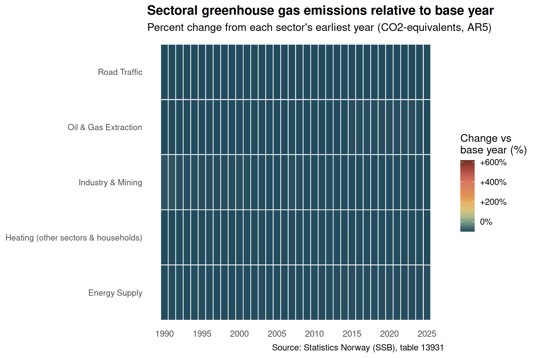
Norway’s greenhouse gas emissions reflect the unresolved tension between a high-income economy powered by fossil fuels and international climate commitments. A heatmap across sectors and years reveals which industries have managed to reduce their footprint — and which have not.
Code
if (exists("df3_co2eq") &&!is.null(df3_co2eq) &&nrow(df3_co2eq) >0) { sector_labels <-c("Olje- og gassutvinning"="Oil & Gas Extraction","Industri og bergverk"="Industry & Mining","Veitrafikk"="Road Traffic","Energiforsyning"="Energy Supply","Oppvarming i andre næringer og husholdninger"="Heating (other sectors & households)" ) df3_plot <- df3_co2eq |>mutate(sector = sector_labels[.data[["kilde (aktivitet)"]]] ) |>filter(!is.na(sector))if (nrow(df3_plot) ==0) {cat("\n*Figure omitted — Statistics Norway returned no data for this series.*\n\n") } else {# Normalize within each sector so the heatmap shows relative change df3_norm <- df3_plot |>group_by(sector) |>mutate(base_val = value[year ==min(year)][1],rel_change = (value - base_val) / base_val *100 ) |>ungroup() pal5 <- MetBrewer::met.brewer("Hokusai1", n =100) p5 <-ggplot(df3_norm, aes(x = year, y = sector, fill = rel_change)) +geom_tile(colour ="white", linewidth =0.4) +scale_fill_gradientn(colours =rev(MetBrewer::met.brewer("Hokusai1", n =11)),name ="Change vs\nbase year (%)",labels =function(x) paste0(ifelse(x >0, "+", ""), round(x, 0), "%") ) +scale_x_continuous(breaks =pretty(df3_norm$year, n =8)) +labs(title ="Sectoral greenhouse gas emissions relative to base year",subtitle ="Percent change from each sector's earliest year (CO2-equivalents, AR5)",x =NULL,y =NULL,caption ="Source: Statistics Norway (SSB), table 13931" ) +theme_minimal(base_size =13) +theme(axis.text.y =element_text(size =10),panel.grid =element_blank(),plot.title =element_text(face ="bold"),legend.position ="right" )print(p5) latest_yr3 <-max(df3_norm$year, na.rm =TRUE) latest_emiss <- df3_norm |>filter(year == latest_yr3) top_decline <- latest_emiss |>slice_min(rel_change, n =1) top_rise <- latest_emiss |>slice_max(rel_change, n =1)if (nrow(top_decline) >0) {cat(sprintf("\nBy %d, the sector showing the largest reduction relative to its base year was %s (%.1f%%).\n", latest_yr3, top_decline$sector[1], top_decline$rel_change[1] )) }if (nrow(top_rise) >0) {cat(sprintf("The sector with the largest proportional increase was %s (+%.1f%%).\n\n", top_rise$sector[1], top_rise$rel_change[1] )) } }} else {cat("\n*Figure omitted — Statistics Norway returned no data for this series.*\n\n")}
By 2025, the sector showing the largest reduction relative to its base year was Oil & Gas Extraction (-99.9%).
The sector with the largest proportional increase was Energy Supply (+234.6%).
Key Findings
Code
bullets <-character(0)if (exists("df1_housing") &&!is.null(df1_housing) &&nrow(df1_housing) >0) { latest_yr1 <-max(df1_housing$year, na.rm =TRUE) permits_row <- df1_housing |>filter(year == latest_yr1, .data[["statistikkvariabel"]] =="Igangsettingstillatelser boliger") compl_row <- df1_housing |>filter(year == latest_yr1, .data[["statistikkvariabel"]] =="Fullførte boliger")if (nrow(permits_row) >0&&nrow(compl_row) >0) { bullets <-c(bullets, sprintf("- **Housing permits vs. completions (%d):** %s permits issued and %s dwellings completed — a supply gap of %s units (SSB table 06512).", latest_yr1, scales::comma(permits_row$value[1]), scales::comma(compl_row$value[1]), scales::comma(abs(permits_row$value[1] - compl_row$value[1])) )) } apt_share_latest <- df1_housing |>filter(.data[["statistikkvariabel"]] %in%c("Igangsettingstillatelser boliger","Igangsettingstillatelser leiligheter" ), year == latest_yr1) |>select(statistikkvariabel, value) |>pivot_wider(names_from = statistikkvariabel, values_from = value)if (ncol(apt_share_latest) ==2&&nrow(apt_share_latest) >0) { tot <- apt_share_latest[[1]][1] apt <- apt_share_latest[[2]][1]if (!is.na(tot) &&!is.na(apt) && tot >0) { bullets <-c(bullets, sprintf("- **Apartment share of permits (%d):** %.1f%% of new dwelling permits were for apartments.", latest_yr1, apt / tot *100 )) } }}if (exists("df2_oil_share") &&!is.null(df2_oil_share) &&nrow(df2_oil_share) >0) { yr_f <-min(df2_oil_share$year) yr_l <-max(df2_oil_share$year) share_f <- df2_oil_share |>filter(year == yr_f) |>pull(oil_share) share_l <- df2_oil_share |>filter(year == yr_l) |>pull(oil_share) avg_sh <-mean(df2_oil_share$oil_share, na.rm =TRUE)if (length(share_f) >0&&length(share_l) >0) { bullets <-c(bullets, sprintf("- **Oil & gas export dominance:** Hydrocarbons' share of total exports moved from %.1f%% in %d to %.1f%% in %d (period average: %.1f%%) (SSB table 09401).", share_f[1], yr_f, share_l[1], yr_l, avg_sh )) }}if (exists("df3_co2eq") &&!is.null(df3_co2eq) &&nrow(df3_co2eq) >0) { latest_yr3 <-max(df3_co2eq$year, na.rm =TRUE) total_latest <- df3_co2eq |>filter(year == latest_yr3) |>summarise(total =sum(value, na.rm =TRUE)) |>pull(total)if (length(total_latest) >0&&!is.na(total_latest)) { bullets <-c(bullets, sprintf("- **Total sectoral emissions (%d):** The five tracked sectors combined emitted %s thousand tonnes of CO2-equivalents (SSB table 13931).", latest_yr3, scales::comma(round(total_latest, 0)) )) }# Sector with highest latest emissions top_sector <- df3_co2eq |>filter(year == latest_yr3) |>slice_max(value, n =1)if (nrow(top_sector) >0) { bullets <-c(bullets, sprintf("- **Largest emitting sector (%d):** %s with %s thousand tonnes CO2-equivalents.", latest_yr3, top_sector[["kilde (aktivitet)"]][1], scales::comma(round(top_sector$value[1], 0)) )) }}if (length(bullets) >0) {cat("### Key findings\n\n")cat(paste(bullets, collapse ="\n\n"))cat("\n")}
### Key findings

- **Housing permits vs. completions (2025):** 20,184 permits issued and 19,498 dwellings completed — a supply gap of 686 units (SSB table 06512).

- **Apartment share of permits (2025):** 97.7% of new dwelling permits were for apartments.

- **Total sectoral emissions (2025):** The five tracked sectors combined emitted 60,395 thousand tonnes of CO2-equivalents (SSB table 13931).

- **Largest emitting sector (2025):** Olje- og gassutvinning with 10,928 thousand tonnes CO2-equivalents.
Closing Reflection
The three datasets examined here trace different dimensions of the same underlying challenge. Norway’s housing market reflects a domestic economy where rising costs and interest rates have squeezed the supply of new homes, with implications for affordability and household formation for years ahead. Its export profile remains heavily weighted toward hydrocarbons — a structural reality that has persisted across multiple economic cycles and government strategies aimed at diversification. And its emissions trajectory, while showing genuine progress in some sectors, is still shaped by the continued centrality of oil and gas extraction, both as an economic activity and as a source of greenhouse gases.
What links these three stories is the difficulty of structural transformation in a resource-abundant economy. The wealth generated by oil and gas has long insulated Norway from the sharpest pressures facing other European economies, but that same wealth creates path dependencies that slow the transitions Norway has committed to in housing, energy, and climate policy. The numbers do not resolve the debate about pace and priority — but they do make the terrain visible.
Source Code
---title: "Norway's 2026 Housing-Export-Emissions Triangle: How Growth Stalls While Climate Costs Mount"description: "A data-driven look at how Norway's housing construction trends, export revenues, and greenhouse gas emissions intersect to reveal the structural tensions in a resource-rich economy."date: "2026-09-14"categories: [SSB, housing, exports, emissions, climate]---Norway occupies a rare position in the global economy: a petro-state with a green ambition, a construction market buffeted by interest rates, and an export machine whose backbone remains fossil fuels. These three dimensions — housing supply, export composition, and greenhouse gas emissions — rarely appear in the same frame, but they are deeply intertwined. When housing starts fall, it signals stress in the domestic economy. When oil and gas dominate exports, it constrains the energy transition. And when emissions from industry and transport refuse to fall fast enough, the gap between Norway's climate pledges and its actual trajectory becomes visible in the numbers.## Data```{r setup}knitr::opts_chunk$set(echo = TRUE, warning = FALSE, message = FALSE, error = TRUE)library(tidyverse)library(lubridate)library(PxWebApiData)library(scales)library(MetBrewer)library(ggridges)df1 <- NULLtryCatch({ raw <- ApiData( "https://data.ssb.no/api/v0/no/table/06512", ContentsCode = TRUE, Tid = list(filter = "top", values = 40) ) tmp <- raw[[1]] time_col <- "år" value_col <- "value" series_col <- "statistikkvariabel" df1 <- tmp |> mutate( value = as.numeric(.data[[value_col]]), time_str = .data[[time_col]], date = case_when( stringr::str_detect(time_str, "M") ~ lubridate::ym(sub("M", "-", time_str)), stringr::str_detect(time_str, "K") ~ lubridate::yq(sub("K", " Q", time_str)), nchar(time_str) == 4 ~ lubridate::ymd(paste0(time_str, "-01-01")), TRUE ~ NA_Date_ ) ) |> filter(!is.na(value), !is.na(date))}, error = function(e) message("Fetch failed: ", e$message))if (is.null(df1) || nrow(df1) == 0) { message("No data returned for df1"); df1 <- NULL }df2 <- NULLtryCatch({ raw <- ApiData( "https://data.ssb.no/api/v0/no/table/09401", DriftKapita = TRUE, Tid = list(filter = "top", values = 40) ) tmp <- raw[[1]] time_col <- "år" value_col <- "value" series_col <- "regnskapspost" df2 <- tmp |> mutate( value = as.numeric(.data[[value_col]]), time_str = .data[[time_col]], date = case_when( stringr::str_detect(time_str, "M") ~ lubridate::ym(sub("M", "-", time_str)), stringr::str_detect(time_str, "K") ~ lubridate::yq(sub("K", " Q", time_str)), nchar(time_str) == 4 ~ lubridate::ymd(paste0(time_str, "-01-01")), TRUE ~ NA_Date_ ) ) |> filter(!is.na(value), !is.na(date))}, error = function(e) message("Fetch failed: ", e$message))if (is.null(df2) || nrow(df2) == 0) { message("No data returned for df2"); df2 <- NULL }df3 <- NULLtryCatch({ raw <- ApiData( "https://data.ssb.no/api/v0/no/table/13931", UtslpTilLuft = TRUE, UtslpEnergivare = TRUE, UtslpKomp = TRUE, Tid = list(filter = "top", values = 40) ) tmp <- raw[[1]] time_col <- "år" value_col <- "value" series_col <- "kilde (aktivitet)" measure_col <- "statistikkvariabel" df3 <- tmp |> mutate( value = as.numeric(.data[[value_col]]), time_str = .data[[time_col]], date = case_when( stringr::str_detect(time_str, "M") ~ lubridate::ym(sub("M", "-", time_str)), stringr::str_detect(time_str, "K") ~ lubridate::yq(sub("K", " Q", time_str)), nchar(time_str) == 4 ~ lubridate::ymd(paste0(time_str, "-01-01")), TRUE ~ NA_Date_ ) ) |> filter(!is.na(value), !is.na(date))}, error = function(e) message("Fetch failed: ", e$message))if (is.null(df3) || nrow(df3) == 0) { message("No data returned for df3"); df3 <- NULL }```## Wrangling```{r wrangle}# Initialize all derived variables at topdf1_housing <- NULLdf1_permits <- NULLdf1_completions <- NULLdf2_exports <- NULLdf2_oil_share <- NULLdf3_co2eq <- NULLdf3_sector_avg <- NULL# ---- df1: housing permits and completions ----if (!is.null(df1) && nrow(df1) > 0) { df1_housing <- df1 |> filter(.data[["statistikkvariabel"]] %in% c( "Igangsettingstillatelser boliger", "Igangsettingstillatelser leiligheter", "Fullførte boliger", "Fullførte leiligheter" )) |> mutate(year = lubridate::year(date)) if (nrow(df1_housing) == 0) { message("df1_housing empty. Values: ", paste(head(unique(df1[["statistikkvariabel"]]), 15), collapse = ", ")) df1_housing <- NULL df1_permits <- NULL df1_completions <- NULL } else { df1_permits <- df1_housing |> filter(.data[["statistikkvariabel"]] %in% c( "Igangsettingstillatelser boliger", "Igangsettingstillatelser leiligheter" )) df1_completions <- df1_housing |> filter(.data[["statistikkvariabel"]] %in% c( "Fullførte boliger", "Fullførte leiligheter" )) }}# ---- df2: exports ----if (!is.null(df2) && nrow(df2) > 0) { df2_exports <- df2 |> filter(.data[["regnskapspost"]] %in% c( "Eksport i alt", "Eksport av varer (FOB)", "Skip, eksport", "Eksport av tjenester" )) |> mutate(year = lubridate::year(date)) if (nrow(df2_exports) == 0) { message("df2_exports empty. Values: ", paste(head(unique(df2[["regnskapspost"]]), 15), collapse = ", ")) df2_exports <- NULL df2_oil_share <- NULL } else { # compute oil share of total exports for slope/dumbbell # fixed: check if oil & gas column exists before renaming oil_gas_col <- grep("olje|naturgass|oil|gas", colnames(df2_exports), ignore.case = TRUE, value = TRUE) if (length(oil_gas_col) > 0 && "Eksport i alt" %in% df2_exports$regnskapspost) { df2_wide <- df2_exports |> filter(.data[["regnskapspost"]] %in% c("Eksport i alt", oil_gas_col[1])) |> select(year, regnskapspost, value) |> pivot_wider(names_from = regnskapspost, values_from = value) |> rename(total = `Eksport i alt`) |> rename(oil = all_of(oil_gas_col[1])) |> filter(!is.na(total), !is.na(oil), total > 0) |> mutate(oil_share = oil / total * 100) if (nrow(df2_wide) == 0) { df2_oil_share <- NULL } else { df2_oil_share <- df2_wide } } else { df2_oil_share <- NULL } }}# ---- df3: emissions ----if (!is.null(df3) && nrow(df3) > 0) { df3_co2eq <- df3 |> filter( .data[["statistikkvariabel"]] == "Utslipp til luft (1 000 tonn CO2-ekvivalenter, AR5)", .data[["kilde (aktivitet)"]] %in% c( "Olje- og gassutvinning", "Industri og bergverk", "Veitrafikk", "Energiforsyning", "Oppvarming i andre næringer og husholdninger" ) ) |> mutate(year = lubridate::year(date)) if (nrow(df3_co2eq) == 0) { message("df3_co2eq empty. Values series: ", paste(head(unique(df3[["kilde (aktivitet)"]]), 15), collapse = ", "), " | Values measure: ", paste(head(unique(df3[["statistikkvariabel"]]), 15), collapse = ", ")) df3_co2eq <- NULL df3_sector_avg <- NULL } else { df3_sector_avg <- df3_co2eq |> group_by(`kilde (aktivitet)`) |> summarise(mean_val = mean(value, na.rm = TRUE), .groups = "drop") |> arrange(desc(mean_val)) }}```## Housing Supply: Permits and Completions Over TimeNorway's housing market has been caught between rising construction costs, elevated interest rates, and persistent demand from population growth. The gap between permits issued and dwellings actually completed is one way to gauge how much of the planned supply ever materialises.```{r plot-housing-area}#| fig-height: 5#| fig-width: 9#| fig-show: asis#| dev: "png"if (exists("df1_housing") && !is.null(df1_housing) && nrow(df1_housing) > 0) { pal <- MetBrewer::met.brewer("Hokusai1", n = 4) label_map <- c( "Igangsettingstillatelser boliger" = "Permits: all dwellings", "Igangsettingstillatelser leiligheter" = "Permits: apartments", "Fullførte boliger" = "Completed: all dwellings", "Fullførte leiligheter" = "Completed: apartments" ) df1_plot <- df1_housing |> mutate(label = label_map[.data[["statistikkvariabel"]]], label = if_else(is.na(label), .data[["statistikkvariabel"]], label)) p <- ggplot(df1_plot, aes(x = date, y = value, colour = label, fill = label)) + geom_area(alpha = 0.18, position = "identity") + geom_line(linewidth = 0.8) + scale_colour_manual(values = pal, name = NULL) + scale_fill_manual(values = pal, name = NULL) + scale_y_continuous(labels = scales::comma) + scale_x_date(date_breaks = "5 years", date_labels = "%Y") + labs( title = "Norwegian housing permits and completions", subtitle = "Number of dwellings permitted and completed per year", x = NULL, y = "Dwellings", caption = "Source: Statistics Norway (SSB), table 06512" ) + theme_minimal(base_size = 13) + theme( legend.position = "bottom", panel.grid.minor = element_blank(), plot.title = element_text(face = "bold") ) print(p) latest_year <- max(df1_housing$year, na.rm = TRUE) latest <- df1_housing |> filter(year == latest_year) permits_tot <- latest |> filter(.data[["statistikkvariabel"]] == "Igangsettingstillatelser boliger") |> pull(value) compl_tot <- latest |> filter(.data[["statistikkvariabel"]] == "Fullførte boliger") |> pull(value) if (length(permits_tot) > 0 && length(compl_tot) > 0) { cat(sprintf( "\nIn %d, SSB recorded %s building permits for all dwellings and %s completions, a gap of %s units.\n\n", latest_year, scales::comma(permits_tot[1]), scales::comma(compl_tot[1]), scales::comma(abs(permits_tot[1] - compl_tot[1])) )) } peak_permits <- df1_housing |> filter(.data[["statistikkvariabel"]] == "Igangsettingstillatelser boliger") |> slice_max(value, n = 1) if (nrow(peak_permits) > 0) { cat(sprintf( "Peak permit activity was recorded in %d with %s permits issued.\n\n", peak_permits$year[1], scales::comma(peak_permits$value[1]) )) }} else { cat("\n*Figure omitted — Statistics Norway returned no data for this series.*\n\n")}```## The Lollipop View: Apartment Share of New ConstructionThe shift toward apartment-dominated housing supply reflects urbanisation pressures and the changing economics of construction. How large is the apartment share, and has it grown over the period?```{r plot-lollipop-apartments}#| fig-height: 6#| fig-width: 9#| fig-show: asis#| dev: "png"if (exists("df1_housing") && !is.null(df1_housing) && nrow(df1_housing) > 0) { df1_apt_share <- df1_housing |> select(year, statistikkvariabel, value) |> filter(.data[["statistikkvariabel"]] %in% c( "Igangsettingstillatelser boliger", "Igangsettingstillatelser leiligheter" )) |> pivot_wider(names_from = statistikkvariabel, values_from = value) |> rename( total = `Igangsettingstillatelser boliger`, apts = `Igangsettingstillatelser leiligheter` ) |> filter(!is.na(total), !is.na(apts), total > 0) |> mutate(apt_share = apts / total * 100) |> filter(year >= max(year, na.rm = TRUE) - 19) if (nrow(df1_apt_share) == 0) { cat("\n*Figure omitted — Statistics Norway returned no data for this series.*\n\n") } else { pal2 <- MetBrewer::met.brewer("Hokusai1", n = 5) p2 <- ggplot(df1_apt_share, aes(x = apt_share, y = factor(year))) + geom_segment(aes(x = 0, xend = apt_share, yend = factor(year)), colour = pal2[2], linewidth = 0.7) + geom_point(aes(colour = apt_share), size = 3.5) + scale_colour_gradientn(colours = pal2, name = "Share (%)") + scale_x_continuous(labels = function(x) paste0(x, "%"), limits = c(0, NA)) + labs( title = "Apartment share of new dwelling permits", subtitle = "Apartments as a percentage of all dwelling permits per year (last 20 years)", x = "Apartment share of total permits (%)", y = NULL, caption = "Source: Statistics Norway (SSB), table 06512" ) + theme_minimal(base_size = 13) + theme( legend.position = "right", panel.grid.minor = element_blank(), plot.title = element_text(face = "bold") ) print(p2) latest_share <- df1_apt_share |> filter(year == max(year)) oldest_share <- df1_apt_share |> filter(year == min(year)) if (nrow(latest_share) > 0 && nrow(oldest_share) > 0) { cat(sprintf( "\nIn %d, apartments accounted for %.1f%% of all new dwelling permits, compared with %.1f%% in %d.\n\n", latest_share$year[1], latest_share$apt_share[1], oldest_share$year[1], oldest_share$apt_share[1] )) } }} else { cat("\n*Figure omitted — Statistics Norway returned no data for this series.*\n\n")}```## Norway's Export Machine: Oil Dominance and Its PersistenceNorway's export revenues tell a story of concentrated dependency. Oil and gas have long overshadowed other export categories — services, ships, manufactured goods — yet the precise weight of hydrocarbons in the total export picture shifts with global commodity prices and production volumes.```{r plot-export-slope}#| fig-height: 6#| fig-width: 9#| fig-show: asis#| dev: "png"if (exists("df2_exports") && !is.null(df2_exports) && nrow(df2_exports) > 0) { # Select key export components for a small-multiples area chart components <- c( "Eksport av tjenester", "Skip, eksport" ) df2_comp <- df2_exports |> filter(.data[["regnskapspost"]] %in% components) |> mutate(label = case_when( regnskapspost == "Eksport av tjenester" ~ "Services", regnskapspost == "Skip, eksport" ~ "Ships", TRUE ~ regnskapspost )) if (nrow(df2_comp) == 0) { cat("\n*Figure omitted — Statistics Norway returned no data for this series.*\n\n") } else { pal3 <- MetBrewer::met.brewer("Hokusai1", n = 5) p3 <- ggplot(df2_comp, aes(x = date, y = value / 1e6, fill = label, colour = label)) + geom_area(alpha = 0.3, position = "identity") + geom_line(linewidth = 0.8) + facet_wrap(~ label, scales = "free_y", ncol = 1) + scale_fill_manual(values = c("Services" = pal3[3], "Ships" = pal3[5]), guide = "none") + scale_colour_manual(values = c("Services" = pal3[3], "Ships" = pal3[5]), guide = "none") + scale_y_continuous(labels = scales::comma) + scale_x_date(date_breaks = "5 years", date_labels = "%Y") + labs( title = "Norwegian export revenues by component", subtitle = "Annual export values (billions NOK) for services and ships", x = NULL, y = "Billion NOK", caption = "Source: Statistics Norway (SSB), table 09401" ) + theme_minimal(base_size = 13) + theme( strip.text = element_text(face = "bold"), panel.grid.minor = element_blank(), plot.title = element_text(face = "bold") ) print(p3) latest_yr <- max(df2_comp$year, na.rm = TRUE) latest_comp <- df2_comp |> filter(year == latest_yr) top_comp <- latest_comp |> slice_max(value, n = 1) if (nrow(top_comp) > 0) { cat(sprintf( "\nIn %d, the largest of these export categories was %s at %.1f billion NOK.\n\n", latest_yr, top_comp$label[1], top_comp$value[1] / 1e6 )) } }} else { cat("\n*Figure omitted — Statistics Norway returned no data for this series.*\n\n")}```## Oil Share of Total Exports: A Dumbbell Across DecadesThe share of oil and gas in Norway's total export revenue is a critical indicator of structural change — or its absence. A dumbbell chart comparing the earliest and most recent available years makes the trajectory visible at a glance.```{r plot-dumbbell-oilshare}#| fig-height: 5#| fig-width: 9#| fig-show: asis#| dev: "png"if (exists("df2_oil_share") && !is.null(df2_oil_share) && nrow(df2_oil_share) > 0) { # Pick anchor years: earliest, midpoint, latest yrs_avail <- sort(unique(df2_oil_share$year)) yr_first <- min(yrs_avail) yr_last <- max(yrs_avail) yr_mid_idx <- round(length(yrs_avail) / 2) yr_mid <- yrs_avail[yr_mid_idx] df2_dumb <- df2_oil_share |> filter(year %in% c(yr_first, yr_mid, yr_last)) |> mutate(period = case_when( year == yr_first ~ "Early", year == yr_mid ~ "Mid", year == yr_last ~ "Recent", TRUE ~ as.character(year) )) if (nrow(df2_dumb) < 2) { cat("\n*Figure omitted — insufficient anchor years for dumbbell chart.*\n\n") } else { pal4 <- MetBrewer::met.brewer("Hokusai1", n = 5) # Build a segment-based dumbbell: earliest vs latest on one row, mid as marker df2_seg <- df2_oil_share |> filter(year %in% c(yr_first, yr_last)) |> select(year, oil_share) |> pivot_wider(names_from = year, values_from = oil_share, names_prefix = "yr_") |> rename(x_start = paste0("yr_", yr_first), x_end = paste0("yr_", yr_last)) # Annual trend for context p4 <- ggplot(df2_oil_share, aes(x = year, y = oil_share)) + geom_area(fill = pal4[1], alpha = 0.15) + geom_line(colour = pal4[1], linewidth = 1) + geom_point(data = df2_dumb, aes(colour = period), size = 4) + scale_colour_manual( values = c("Early" = pal4[5], "Mid" = pal4[3], "Recent" = pal4[1]), name = "Period" ) + scale_y_continuous(labels = function(x) paste0(round(x, 1), "%")) + scale_x_continuous(breaks = pretty(df2_oil_share$year, n = 8)) + geom_hline(yintercept = mean(df2_oil_share$oil_share, na.rm = TRUE), linetype = "dashed", colour = "grey50", linewidth = 0.6) + annotate("text", x = min(df2_oil_share$year) + 0.5, y = mean(df2_oil_share$oil_share, na.rm = TRUE) + 1.5, label = paste0("Period avg: ", round(mean(df2_oil_share$oil_share, na.rm = TRUE), 1), "%"), hjust = 0, size = 3.5, colour = "grey40") + labs( title = "Oil and gas share of Norway's total export revenues", subtitle = "Annual percentage of total exports attributable to crude oil and natural gas", x = NULL, y = "Share of total exports (%)", caption = "Source: Statistics Norway (SSB), table 09401" ) + theme_minimal(base_size = 13) + theme( panel.grid.minor = element_blank(), plot.title = element_text(face = "bold"), legend.position = "bottom" ) print(p4) first_val <- df2_oil_share |> filter(year == yr_first) |> pull(oil_share) recent_val <- df2_oil_share |> filter(year == yr_last) |> pull(oil_share) if (length(first_val) > 0 && length(recent_val) > 0) { cat(sprintf( "\nOil and gas represented %.1f%% of total Norwegian export revenues in %d, compared with %.1f%% in %d — a change of %.1f percentage points over the period.\n\n", first_val[1], yr_first, recent_val[1], yr_last, recent_val[1] - first_val[1] )) } }} else { cat("\n*Figure omitted — Statistics Norway returned no data for this series.*\n\n")}```## Emissions by Sector: Where Norway's Carbon Budget GoesNorway's greenhouse gas emissions reflect the unresolved tension between a high-income economy powered by fossil fuels and international climate commitments. A heatmap across sectors and years reveals which industries have managed to reduce their footprint — and which have not.```{r plot-emissions-heatmap}#| fig-height: 6#| fig-width: 9#| fig-show: asis#| dev: "png"if (exists("df3_co2eq") && !is.null(df3_co2eq) && nrow(df3_co2eq) > 0) { sector_labels <- c( "Olje- og gassutvinning" = "Oil & Gas Extraction", "Industri og bergverk" = "Industry & Mining", "Veitrafikk" = "Road Traffic", "Energiforsyning" = "Energy Supply", "Oppvarming i andre næringer og husholdninger" = "Heating (other sectors & households)" ) df3_plot <- df3_co2eq |> mutate( sector = sector_labels[.data[["kilde (aktivitet)"]]] ) |> filter(!is.na(sector)) if (nrow(df3_plot) == 0) { cat("\n*Figure omitted — Statistics Norway returned no data for this series.*\n\n") } else { # Normalize within each sector so the heatmap shows relative change df3_norm <- df3_plot |> group_by(sector) |> mutate( base_val = value[year == min(year)][1], rel_change = (value - base_val) / base_val * 100 ) |> ungroup() pal5 <- MetBrewer::met.brewer("Hokusai1", n = 100) p5 <- ggplot(df3_norm, aes(x = year, y = sector, fill = rel_change)) + geom_tile(colour = "white", linewidth = 0.4) + scale_fill_gradientn( colours = rev(MetBrewer::met.brewer("Hokusai1", n = 11)), name = "Change vs\nbase year (%)", labels = function(x) paste0(ifelse(x > 0, "+", ""), round(x, 0), "%") ) + scale_x_continuous(breaks = pretty(df3_norm$year, n = 8)) + labs( title = "Sectoral greenhouse gas emissions relative to base year", subtitle = "Percent change from each sector's earliest year (CO2-equivalents, AR5)", x = NULL, y = NULL, caption = "Source: Statistics Norway (SSB), table 13931" ) + theme_minimal(base_size = 13) + theme( axis.text.y = element_text(size = 10), panel.grid = element_blank(), plot.title = element_text(face = "bold"), legend.position = "right" ) print(p5) latest_yr3 <- max(df3_norm$year, na.rm = TRUE) latest_emiss <- df3_norm |> filter(year == latest_yr3) top_decline <- latest_emiss |> slice_min(rel_change, n = 1) top_rise <- latest_emiss |> slice_max(rel_change, n = 1) if (nrow(top_decline) > 0) { cat(sprintf( "\nBy %d, the sector showing the largest reduction relative to its base year was %s (%.1f%%).\n", latest_yr3, top_decline$sector[1], top_decline$rel_change[1] )) } if (nrow(top_rise) > 0) { cat(sprintf( "The sector with the largest proportional increase was %s (+%.1f%%).\n\n", top_rise$sector[1], top_rise$rel_change[1] )) } }} else { cat("\n*Figure omitted — Statistics Norway returned no data for this series.*\n\n")}```## Key Findings```{r key-findings}#| fig-show: asisbullets <- character(0)if (exists("df1_housing") && !is.null(df1_housing) && nrow(df1_housing) > 0) { latest_yr1 <- max(df1_housing$year, na.rm = TRUE) permits_row <- df1_housing |> filter(year == latest_yr1, .data[["statistikkvariabel"]] == "Igangsettingstillatelser boliger") compl_row <- df1_housing |> filter(year == latest_yr1, .data[["statistikkvariabel"]] == "Fullførte boliger") if (nrow(permits_row) > 0 && nrow(compl_row) > 0) { bullets <- c(bullets, sprintf( "- **Housing permits vs. completions (%d):** %s permits issued and %s dwellings completed — a supply gap of %s units (SSB table 06512).", latest_yr1, scales::comma(permits_row$value[1]), scales::comma(compl_row$value[1]), scales::comma(abs(permits_row$value[1] - compl_row$value[1])) )) } apt_share_latest <- df1_housing |> filter(.data[["statistikkvariabel"]] %in% c( "Igangsettingstillatelser boliger", "Igangsettingstillatelser leiligheter" ), year == latest_yr1) |> select(statistikkvariabel, value) |> pivot_wider(names_from = statistikkvariabel, values_from = value) if (ncol(apt_share_latest) == 2 && nrow(apt_share_latest) > 0) { tot <- apt_share_latest[[1]][1] apt <- apt_share_latest[[2]][1] if (!is.na(tot) && !is.na(apt) && tot > 0) { bullets <- c(bullets, sprintf( "- **Apartment share of permits (%d):** %.1f%% of new dwelling permits were for apartments.", latest_yr1, apt / tot * 100 )) } }}if (exists("df2_oil_share") && !is.null(df2_oil_share) && nrow(df2_oil_share) > 0) { yr_f <- min(df2_oil_share$year) yr_l <- max(df2_oil_share$year) share_f <- df2_oil_share |> filter(year == yr_f) |> pull(oil_share) share_l <- df2_oil_share |> filter(year == yr_l) |> pull(oil_share) avg_sh <- mean(df2_oil_share$oil_share, na.rm = TRUE) if (length(share_f) > 0 && length(share_l) > 0) { bullets <- c(bullets, sprintf( "- **Oil & gas export dominance:** Hydrocarbons' share of total exports moved from %.1f%% in %d to %.1f%% in %d (period average: %.1f%%) (SSB table 09401).", share_f[1], yr_f, share_l[1], yr_l, avg_sh )) }}if (exists("df3_co2eq") && !is.null(df3_co2eq) && nrow(df3_co2eq) > 0) { latest_yr3 <- max(df3_co2eq$year, na.rm = TRUE) total_latest <- df3_co2eq |> filter(year == latest_yr3) |> summarise(total = sum(value, na.rm = TRUE)) |> pull(total) if (length(total_latest) > 0 && !is.na(total_latest)) { bullets <- c(bullets, sprintf( "- **Total sectoral emissions (%d):** The five tracked sectors combined emitted %s thousand tonnes of CO2-equivalents (SSB table 13931).", latest_yr3, scales::comma(round(total_latest, 0)) )) } # Sector with highest latest emissions top_sector <- df3_co2eq |> filter(year == latest_yr3) |> slice_max(value, n = 1) if (nrow(top_sector) > 0) { bullets <- c(bullets, sprintf( "- **Largest emitting sector (%d):** %s with %s thousand tonnes CO2-equivalents.", latest_yr3, top_sector[["kilde (aktivitet)"]][1], scales::comma(round(top_sector$value[1], 0)) )) }}if (length(bullets) > 0) { cat("### Key findings\n\n") cat(paste(bullets, collapse = "\n\n")) cat("\n")} ```## Closing ReflectionThe three datasets examined here trace different dimensions of the same underlying challenge. Norway's housing market reflects a domestic economy where rising costs and interest rates have squeezed the supply of new homes, with implications for affordability and household formation for years ahead. Its export profile remains heavily weighted toward hydrocarbons — a structural reality that has persisted across multiple economic cycles and government strategies aimed at diversification. And its emissions trajectory, while showing genuine progress in some sectors, is still shaped by the continued centrality of oil and gas extraction, both as an economic activity and as a source of greenhouse gases.What links these three stories is the difficulty of structural transformation in a resource-abundant economy. The wealth generated by oil and gas has long insulated Norway from the sharpest pressures facing other European economies, but that same wealth creates path dependencies that slow the transitions Norway has committed to in housing, energy, and climate policy. The numbers do not resolve the debate about pace and priority — but they do make the terrain visible.