Three independent data streams — freight transport volumes, petroleum product sales, and household living arrangements — converge to sketch a portrait of an economy under quiet but compounding pressure.
Published
September 8, 2026
Norway’s economic resilience has long rested on interlocking pillars: efficient logistics networks moving raw materials and manufactured goods, a transport fuel market calibrated to industrial demand, and a social structure of stable households. When all three show signs of strain simultaneously, the cumulative signal deserves close attention. This post draws on three SSB datasets — quarterly freight transport, monthly petroleum sales, and annual data on living arrangements — to ask whether 2026 marks a structural inflection point or a cyclical wobble.
The Freight Squeeze: What Norway Ships and How Far
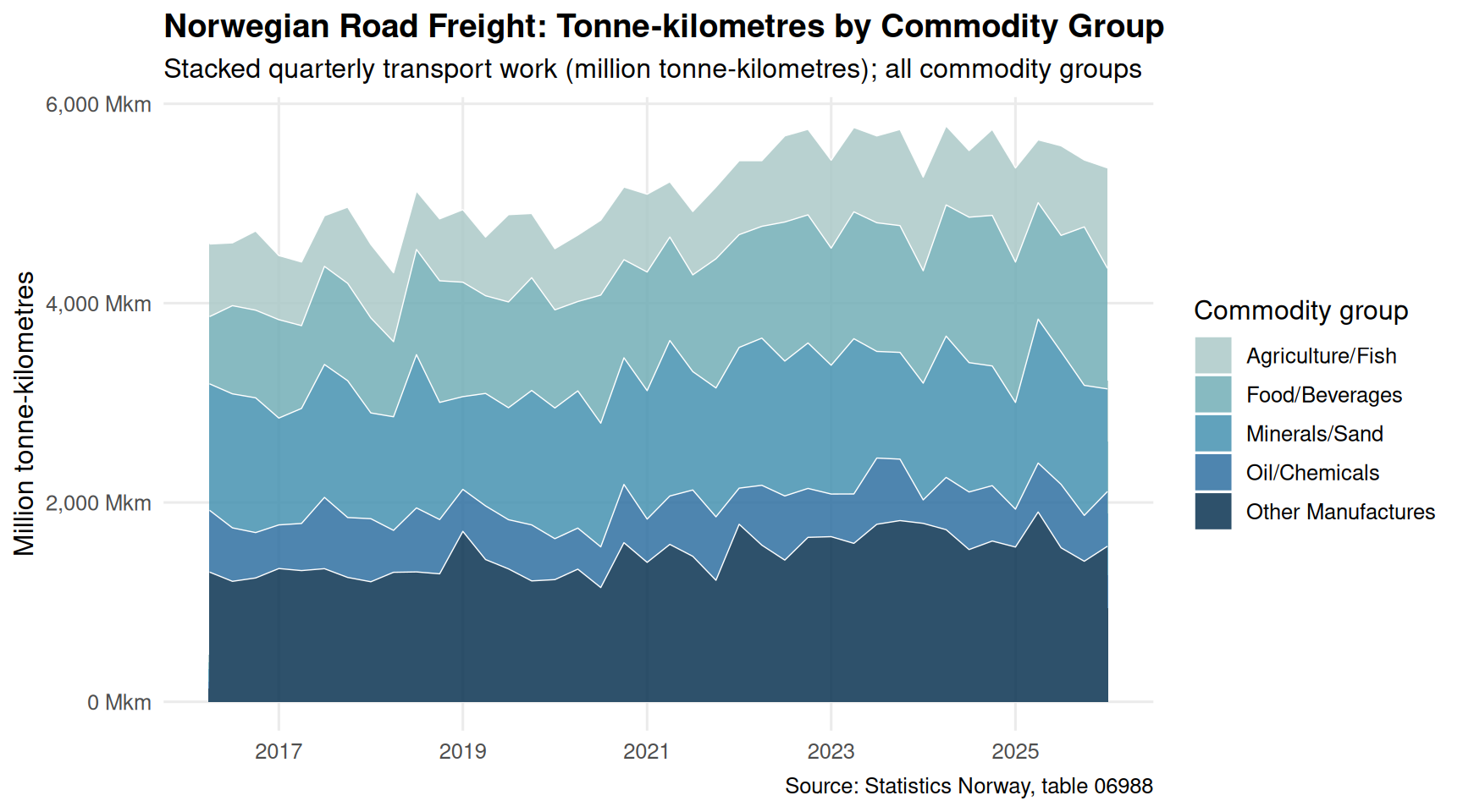
Freight transport is one of the economy’s most direct pulse-checks. A slowdown in tonne-kilometres moved signals that supply chains are shortening, demand is weakening, or both. Norway’s commodity mix — agricultural products, processed food, oil-linked chemicals, and minerals — tells a story about which sectors are still driving physical flows.
Code
if (exists("df1_work") &&!is.null(df1_work) &&nrow(df1_work) >0) { pal <-met.brewer("Hokusai2", n =length(unique(df1_work$vareslag_short))) p <-ggplot(df1_work,aes(x = date, y = value, fill = vareslag_short)) +geom_area(alpha =0.85, colour ="white", linewidth =0.25) +scale_fill_manual(values = pal, name ="Commodity group") +scale_x_date(date_breaks ="2 years", date_labels ="%Y") +scale_y_continuous(labels =comma_format(suffix =" Mkm")) +labs(title ="Norwegian Road Freight: Tonne-kilometres by Commodity Group",subtitle ="Stacked quarterly transport work (million tonne-kilometres); all commodity groups",caption ="Source: Statistics Norway, table 06988",x =NULL, y ="Million tonne-kilometres" ) +theme_minimal(base_size =12) +theme(legend.position ="right",panel.grid.minor =element_blank(),plot.title =element_text(face ="bold") )print(p) latest_q <-max(df1_work$date) total_now <- df1_work |>filter(date == latest_q) |>summarise(tot =sum(value, na.rm =TRUE)) |>pull(tot) top_seg <- df1_work |>filter(date == latest_q) |>slice_max(value, n =1)cat(sprintf("\nIn the most recent quarter (%s), total road freight work reached %.1f million tonne-kilometres. The largest single commodity group was '%s', accounting for %.1f million tonne-kilometres.\n\n",format(latest_q, "%Y Q%q"), total_now, top_seg$vareslag_short[1], top_seg$value[1] ))} else {cat("\n*Figure omitted — Statistics Norway returned no data for this series.*\n\n")}
In the most recent quarter (2026 Q%q), total road freight work reached 5357.0 million tonne-kilometres. The largest single commodity group was 'Other Manufactures', accounting for 1561.1 million tonne-kilometres.
Code
if (exists("df1_heatmap") &&!is.null(df1_heatmap) &&nrow(df1_heatmap) >0) { df1_heatmap_plot <- df1_heatmap |>filter(!is.na(year), !is.na(qtr)) p <-ggplot(df1_heatmap_plot,aes(x =factor(year), y = qtr, fill = value)) +geom_tile(colour ="white", linewidth =0.4) +facet_wrap(~ vareslag_short, ncol =2) +scale_fill_gradientn(colours =met.brewer("Hiroshige", 9),name ="Mill. tonnes",labels =comma_format() ) +labs(title ="Freight Volume Intensity by Commodity and Quarter",subtitle ="Transport tonnage (million tonnes) per quarter; darker = higher volume",caption ="Source: Statistics Norway, table 06988",x =NULL, y ="Quarter" ) +theme_minimal(base_size =11) +theme(axis.text.x =element_text(angle =45, hjust =1, size =8),strip.text =element_text(face ="bold", size =9),panel.grid =element_blank(),plot.title =element_text(face ="bold"),legend.position ="right" )print(p) peak_row <- df1_heatmap_plot |>slice_max(value, n =1)cat(sprintf("\nThe highest single quarter-commodity cell in the heatmap corresponds to '%s' in %d %s, at %.2f million tonnes.\n\n", peak_row$vareslag_short[1], peak_row$year[1], peak_row$qtr[1], peak_row$value[1] ))} else {cat("\n*Figure omitted — Statistics Norway returned no data for this series.*\n\n")}
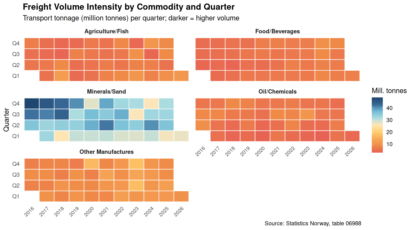
The highest single quarter-commodity cell in the heatmap corresponds to 'Minerals/Sand' in 2016 Q4, at 48.70 million tonnes.
Pump Sales in Decline: Norway’s Shifting Fuel Landscape
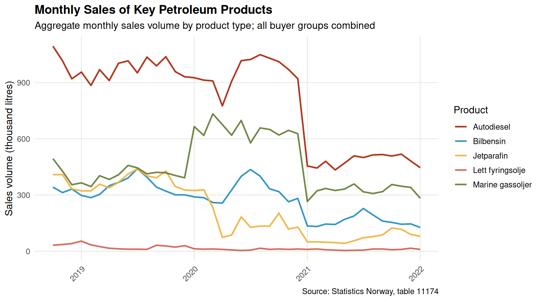
Petroleum product sales track not just consumer behaviour but the broader rhythm of Norwegian industry and mobility. Diesel demand reflects construction and logistics; petrol captures private motoring; jet fuel signals aviation recovery; marine gas oils tell us about fisheries and coastal shipping. Shifts in these curves carry outsized economic meaning.
Code
if (exists("df2_main") &&!is.null(df2_main) &&nrow(df2_main) >0) { pal2 <-met.brewer("Juarez", n =length(unique(df2_main$petroleumsprodukt))) p <-ggplot(df2_main,aes(x = date, y = value, colour = petroleumsprodukt,group = petroleumsprodukt)) +geom_line(linewidth =0.9, alpha =0.9) +scale_colour_manual(values = pal2, name ="Product") +scale_x_date(date_breaks ="1 year", date_labels ="%Y") +scale_y_continuous(labels =comma_format()) +labs(title ="Monthly Sales of Key Petroleum Products",subtitle ="Aggregate monthly sales volume by product type; all buyer groups combined",caption ="Source: Statistics Norway, table 11174",x =NULL, y ="Sales volume (thousand litres)" ) +theme_minimal(base_size =12) +theme(legend.position ="right",panel.grid.minor =element_blank(),axis.text.x =element_text(angle =45, hjust =1),plot.title =element_text(face ="bold") )print(p) latest_m <-max(df2_main$date) top_prod <- df2_main |>filter(date == latest_m) |>slice_max(value, n =1) low_prod <- df2_main |>filter(date == latest_m) |>slice_min(value, n =1)cat(sprintf("\nIn %s (the most recent month), '%s' recorded the highest sales at %s thousand litres, while '%s' recorded the lowest at %s thousand litres.\n\n",format(latest_m, "%B %Y"), top_prod$petroleumsprodukt[1],comma(round(top_prod$value[1])), low_prod$petroleumsprodukt[1],comma(round(low_prod$value[1])) ))} else {cat("\n*Figure omitted — Statistics Norway returned no data for this series.*\n\n")}
In January 2022 (the most recent month), 'Autodiesel' recorded the highest sales at 446 thousand litres, while 'Lett fyringsolje' recorded the lowest at 10 thousand litres.
Code
if (exists("df2_seasonal") &&!is.null(df2_seasonal) &&nrow(df2_seasonal) >0) { pal3 <-met.brewer("Juarez", n =length(unique(df2_seasonal$petroleumsprodukt))) p <-ggplot(df2_seasonal,aes(x = value, y = month, fill = petroleumsprodukt)) +geom_density_ridges(alpha =0.65, scale =1.3, rel_min_height =0.01,colour ="white", linewidth =0.4) +facet_wrap(~ petroleumsprodukt, ncol =1, scales ="free_x") +scale_fill_manual(values = pal3, guide ="none") +scale_x_continuous(labels =comma_format()) +labs(title ="Seasonal Distribution of Road Fuel Sales by Month",subtitle ="Ridgeline densities of monthly sales volume; petrol, auto-diesel, construction diesel",caption ="Source: Statistics Norway, table 11174",x ="Sales volume (thousand litres)", y =NULL ) +theme_minimal(base_size =11) +theme(strip.text =element_text(face ="bold"),panel.grid.minor =element_blank(),plot.title =element_text(face ="bold") )print(p) peak_month <- df2_seasonal |>group_by(petroleumsprodukt, month) |>summarise(avg_val =mean(value, na.rm =TRUE), .groups ="drop") |>group_by(petroleumsprodukt) |>slice_max(avg_val, n =1)for (i inseq_len(nrow(peak_month))) {cat(sprintf("\nFor '%s', the month with the highest average sales is %s (avg %.0f thousand litres).", peak_month$petroleumsprodukt[i],as.character(peak_month$month[i]), peak_month$avg_val[i] )) }cat("\n\n")} else {cat("\n*Figure omitted — Statistics Norway returned no data for this series.*\n\n")}
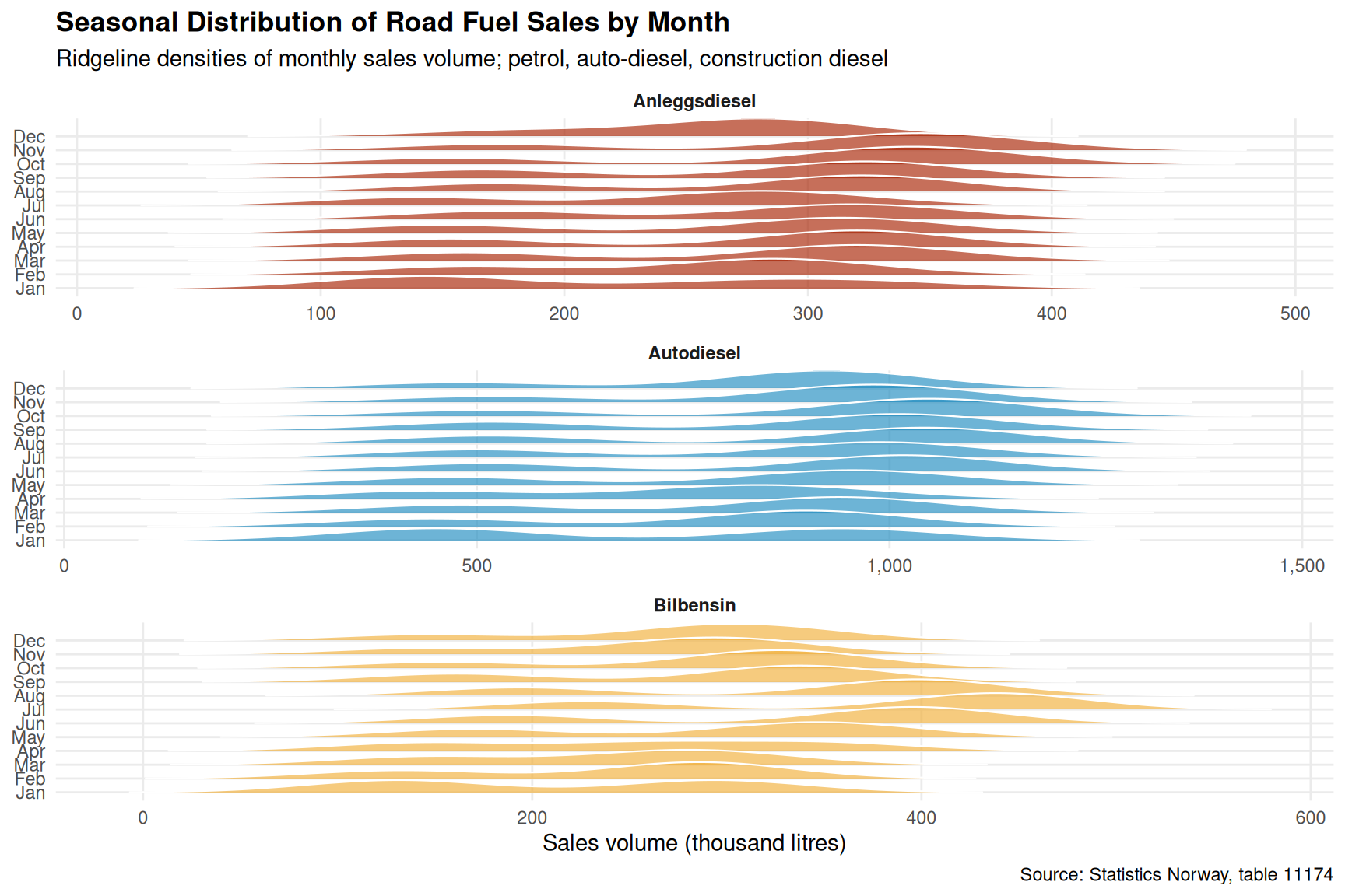
For 'Anleggsdiesel', the month with the highest average sales is Nov (avg 303 thousand litres).
For 'Autodiesel', the month with the highest average sales is Oct (avg 913 thousand litres).
For 'Bilbensin', the month with the highest average sales is Jul (avg 368 thousand litres).
Household Fragmentation: The Quiet Demographic Shift
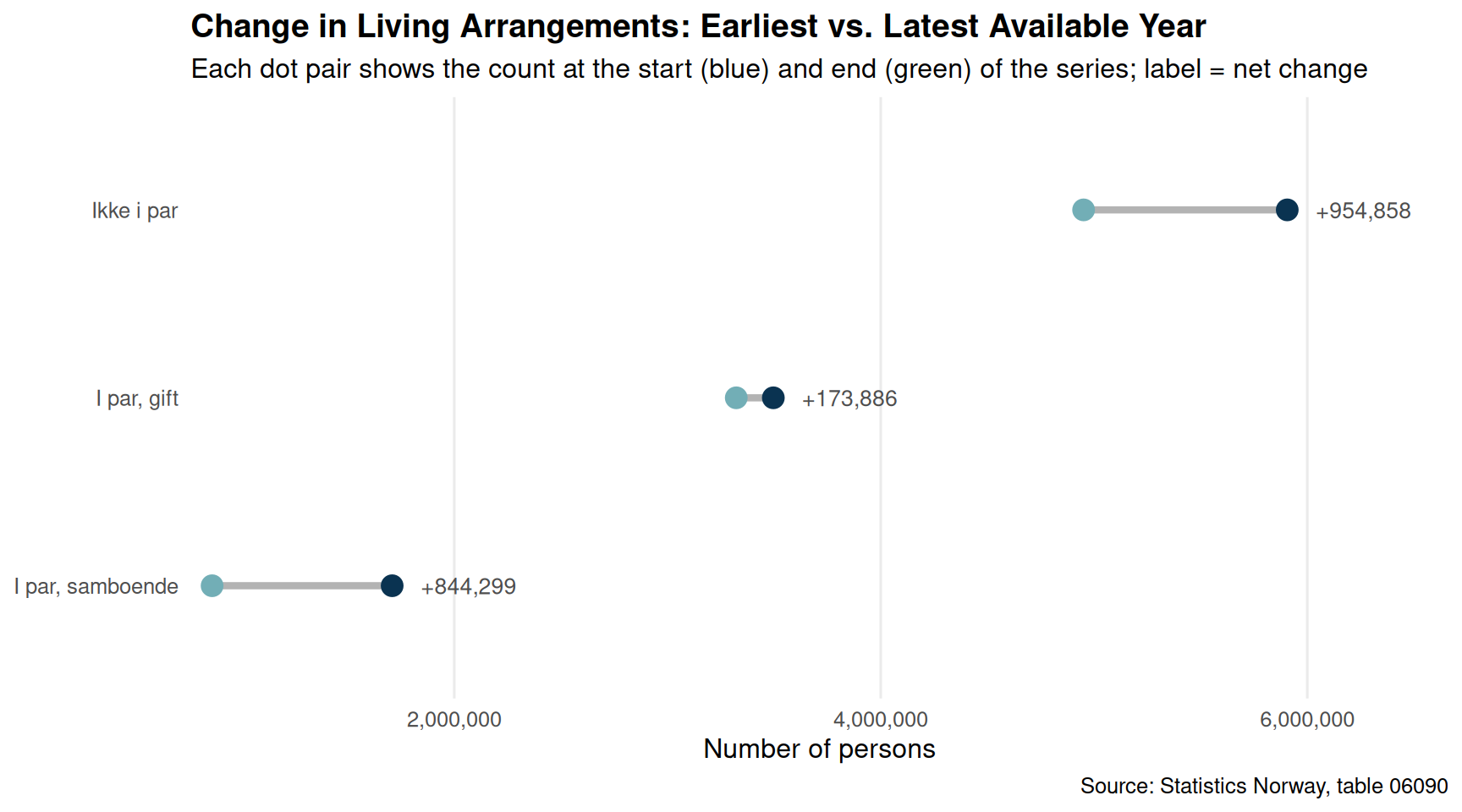
Behind every economic indicator is a household making decisions about work, spending, and debt. The shift away from marriage toward cohabitation and, crucially, living alone, has profound implications for housing demand, consumption patterns, and social resilience. SSB’s data on living arrangements offer a window into this long-run structural change.
Code
if (exists("df3_dumbbell") &&!is.null(df3_dumbbell) &&nrow(df3_dumbbell) >0) { df3_db_wide <- df3_dumbbell |>pivot_wider(names_from = period, values_from = value) |>filter(!is.na(Earliest) &!is.na(Latest)) |>mutate(change = Latest - Earliest,samlivsform =fct_reorder(samlivsform, Latest))if (nrow(df3_db_wide) >0) { pal4 <-met.brewer("Hokusai2", 3) p <-ggplot(df3_db_wide) +geom_segment(aes(x = Earliest, xend = Latest,y = samlivsform, yend = samlivsform),colour ="grey70", linewidth =1.5) +geom_point(aes(x = Earliest, y = samlivsform),colour = pal4[1], size =4) +geom_point(aes(x = Latest, y = samlivsform),colour = pal4[3], size =4) +geom_text(aes(x = Latest, y = samlivsform,label =if_else(change >=0,paste0("+", comma(round(change))),comma(round(change)))),hjust =-0.3, size =3.5, colour ="grey30") +scale_x_continuous(labels =comma_format(), expand =expansion(mult =c(0.02, 0.15))) +labs(title ="Change in Living Arrangements: Earliest vs. Latest Available Year",subtitle ="Each dot pair shows the count at the start (blue) and end (green) of the series; label = net change",caption ="Source: Statistics Norway, table 06090",x ="Number of persons", y =NULL ) +theme_minimal(base_size =12) +theme(panel.grid.minor =element_blank(),panel.grid.major.y =element_blank(),plot.title =element_text(face ="bold") )print(p) largest_gain <- df3_db_wide |>slice_max(change, n =1) largest_loss <- df3_db_wide |>slice_min(change, n =1)cat(sprintf("\nThe living arrangement with the largest absolute increase is '%s' (+%s persons). The largest decrease is in '%s' (%s persons).\n\n", largest_gain$samlivsform[1],comma(round(largest_gain$change[1])), largest_loss$samlivsform[1],comma(round(largest_loss$change[1])) )) }} else {cat("\n*Figure omitted — Statistics Norway returned no data for this series.*\n\n")}
The living arrangement with the largest absolute increase is 'Ikke i par' (+954,858 persons). The largest decrease is in 'I par, gift' (173,886 persons).
Key Findings
Code
bullets <-character(0)if (!is.null(df1) &&nrow(df1) >0&&!is.null(df1_work) &&nrow(df1_work) >0) { latest_q <-max(df1_work$date) total_now <- df1_work |>filter(date == latest_q) |>summarise(tot =sum(value, na.rm =TRUE)) |>pull(tot) top_seg <- df1_work |>filter(date == latest_q) |>slice_max(value, n =1) n_qtrs <-n_distinct(df1_work$date) bullets <-c(bullets, sprintf("**Freight transport (table 06988):** Over %d quarters of data, the most recent quarter (%s) recorded %.1f million tonne-kilometres of total road freight work. The dominant commodity group was '%s' at %.1f million tonne-kilometres.", n_qtrs,format(latest_q, "%Y Q%q"), total_now, top_seg$vareslag_short[1], top_seg$value[1] ))}if (!is.null(df2) &&nrow(df2) >0&&!is.null(df2_main) &&nrow(df2_main) >0) { latest_m <-max(df2_main$date) top_prod <- df2_main |>filter(date == latest_m) |>slice_max(value, n =1) n_months <-n_distinct(df2_main$date) bullets <-c(bullets, sprintf("**Petroleum sales (table 11174):** The series spans %d monthly observations. In %s, the highest-selling product was '%s' at %s thousand litres.", n_months,format(latest_m, "%B %Y"), top_prod$petroleumsprodukt[1],comma(round(top_prod$value[1])) ))}if (!is.null(df3) &&nrow(df3) >0&&!is.null(df3_dumbbell) &&nrow(df3_dumbbell) >0) { df3_db_wide2 <- df3_dumbbell |>pivot_wider(names_from = period, values_from = value) |>filter(!is.na(Earliest) &!is.na(Latest)) |>mutate(change = Latest - Earliest)if (nrow(df3_db_wide2) >0) { largest_gain2 <- df3_db_wide2 |>slice_max(change, n =1) bullets <-c(bullets, sprintf("**Living arrangements (table 06090):** Across all recorded years, the arrangement type showing the greatest growth is '%s', which added %s persons between the earliest and most recent available year.", largest_gain2$samlivsform[1],comma(round(largest_gain2$change[1])) )) }}if (length(bullets) >0) {cat("### Key findings\n\n")for (b in bullets) {cat("-", b, "\n\n") }} else {cat("*No data were available for key findings.*\n\n")}
### Key findings

- **Freight transport (table 06988):** Over 40 quarters of data, the most recent quarter (2026 Q%q) recorded 5357.0 million tonne-kilometres of total road freight work. The dominant commodity group was 'Other Manufactures' at 1561.1 million tonne-kilometres.

- **Petroleum sales (table 11174):** The series spans 40 monthly observations. In January 2022, the highest-selling product was 'Autodiesel' at 446 thousand litres.

- **Living arrangements (table 06090):** Across all recorded years, the arrangement type showing the greatest growth is 'Ikke i par', which added 954,858 persons between the earliest and most recent available year.
Closing Reflection
Norway enters the second half of 2026 navigating pressures that, individually, might be dismissed as routine cyclical noise. Together, however — shifting freight volumes across commodity classes, evolving petroleum consumption patterns, and a steady long-run transformation in how Norwegians organise their domestic lives — they suggest that the structural underpinnings of Norwegian economic life are in genuine flux. The logistics sector adjusts to demand signals that originate far upstream; fuel markets reflect both technological transitions and underlying economic activity; and household fragmentation quietly reshapes every downstream social statistic from housing demand to savings rates. Tracking these three dimensions together offers a richer diagnostic than any single indicator can provide.
Source Code
---title: "Norway's 2026 Structural Stress Test: Logistics, Fuel, and Household Fragmentation"description: "Three independent data streams — freight transport volumes, petroleum product sales, and household living arrangements — converge to sketch a portrait of an economy under quiet but compounding pressure."date: "2026-09-08"categories: [SSB, transport, energy, demographics]---Norway's economic resilience has long rested on interlocking pillars: efficient logistics networks moving raw materials and manufactured goods, a transport fuel market calibrated to industrial demand, and a social structure of stable households. When all three show signs of strain simultaneously, the cumulative signal deserves close attention. This post draws on three SSB datasets — quarterly freight transport, monthly petroleum sales, and annual data on living arrangements — to ask whether 2026 marks a structural inflection point or a cyclical wobble.```{r setup}knitr::opts_chunk$set(echo = TRUE, warning = FALSE, message = FALSE, error = TRUE)library(tidyverse)library(lubridate)library(PxWebApiData)library(scales)library(ggridges)library(MetBrewer)df1 <- NULLtryCatch({ raw <- ApiData( "https://data.ssb.no/api/v0/no/table/06988", Vareslag = TRUE, ContentsCode = TRUE, Tid = list(filter = "top", values = 40) ) tmp <- raw[[1]] time_col <- "kvartal" value_col <- "value" series_col <- "vareslag" measure_col <- "statistikkvariabel" df1 <- tmp |> mutate( value = as.numeric(.data[[value_col]]), time_str = .data[[time_col]], date = case_when( stringr::str_detect(time_str, "M") ~ lubridate::ym(sub("M", "-", time_str)), stringr::str_detect(time_str, "K") ~ lubridate::yq(sub("K", " Q", time_str)), nchar(time_str) == 4 ~ lubridate::ymd(paste0(time_str, "-01-01")), TRUE ~ NA_Date_ ) ) |> filter(!is.na(value), !is.na(date)) if (is.null(df1) || nrow(df1) == 0) { message("No data returned for df1"); df1 <- NULL }}, error = function(e) message("Fetch failed: ", e$message))df2 <- NULLtryCatch({ raw <- ApiData( "https://data.ssb.no/api/v0/no/table/11174", Region = TRUE, Kjopegrupper = TRUE, PetroleumProd = TRUE, ContentsCode = TRUE, Tid = list(filter = "top", values = 40) ) tmp <- raw[[1]] time_col <- "måned" value_col <- "value" series_col <- "petroleumsprodukt" measure_col <- "statistikkvariabel" df2 <- tmp |> mutate( value = as.numeric(.data[[value_col]]), time_str = .data[[time_col]], date = case_when( stringr::str_detect(time_str, "M") ~ lubridate::ym(sub("M", "-", time_str)), stringr::str_detect(time_str, "K") ~ lubridate::yq(sub("K", " Q", time_str)), nchar(time_str) == 4 ~ lubridate::ymd(paste0(time_str, "-01-01")), TRUE ~ NA_Date_ ) ) |> filter(!is.na(value), !is.na(date)) if (is.null(df2) || nrow(df2) == 0) { message("No data returned for df2"); df2 <- NULL }}, error = function(e) message("Fetch failed: ", e$message))df3 <- NULLtryCatch({ raw <- ApiData( "https://data.ssb.no/api/v0/no/table/06090", Kjonn = TRUE, Samlivsform = TRUE, Alder = TRUE, Tid = list(filter = "top", values = 40) ) tmp <- raw[[1]] time_col <- "år" value_col <- "value" series_col <- "samlivsform" df3 <- tmp |> mutate( value = as.numeric(.data[[value_col]]), time_str = .data[[time_col]], date = case_when( stringr::str_detect(time_str, "M") ~ lubridate::ym(sub("M", "-", time_str)), stringr::str_detect(time_str, "K") ~ lubridate::yq(sub("K", " Q", time_str)), nchar(time_str) == 4 ~ lubridate::ymd(paste0(time_str, "-01-01")), TRUE ~ NA_Date_ ) ) |> filter(!is.na(value), !is.na(date)) if (is.null(df3) || nrow(df3) == 0) { message("No data returned for df3"); df3 <- NULL }}, error = function(e) message("Fetch failed: ", e$message))```## Wrangling```{r wrangle}# ── df1: freight transport ────────────────────────────────────────────────────df1_tonnage <- NULLdf1_work <- NULLdf1_heatmap <- NULLif (!is.null(df1) && nrow(df1) > 0) { df1_tonnage <- df1 |> filter(.data[["statistikkvariabel"]] == "Transportmengde (mill. tonn)") |> filter(.data[["vareslag"]] != "") |> mutate(vareslag_short = case_when( str_detect(vareslag, "Jordbruks") ~ "Agriculture/Fish", str_detect(vareslag, "Nærings") ~ "Food/Beverages", str_detect(vareslag, "Kull") ~ "Oil/Chemicals", str_detect(vareslag, "Malm") ~ "Minerals/Sand", str_detect(vareslag, "Andre") ~ "Other Manufactures", TRUE ~ vareslag )) df1_work <- df1 |> filter(.data[["statistikkvariabel"]] == "Transportarbeid (mill. tonnkm)") |> filter(.data[["vareslag"]] != "") |> mutate(vareslag_short = case_when( str_detect(vareslag, "Jordbruks") ~ "Agriculture/Fish", str_detect(vareslag, "Nærings") ~ "Food/Beverages", str_detect(vareslag, "Kull") ~ "Oil/Chemicals", str_detect(vareslag, "Malm") ~ "Minerals/Sand", str_detect(vareslag, "Andre") ~ "Other Manufactures", TRUE ~ vareslag )) df1_heatmap <- df1_tonnage |> mutate( year = year(date), qtr = paste0("Q", quarter(date)) ) |> group_by(vareslag_short, year, qtr) |> summarise(value = sum(value, na.rm = TRUE), .groups = "drop")}# ── df2: petroleum product sales ─────────────────────────────────────────────df2_main <- NULLdf2_seasonal <- NULLdf2_lollipop <- NULLif (!is.null(df2) && nrow(df2) > 0) { has_monthly <- any(stringr::str_detect(df2$time_str, "M\\d{2}"), na.rm = TRUE) df2_main <- df2 |> filter(.data[["petroleumsprodukt"]] %in% c( "Bilbensin", "Autodiesel", "Jetparafin", "Marine gassoljer", "Lett fyringsolje" )) |> group_by(petroleumsprodukt, date) |> summarise(value = sum(value, na.rm = TRUE), .groups = "drop") if (has_monthly) { df2_seasonal <- df2 |> filter(.data[["petroleumsprodukt"]] %in% c( "Bilbensin", "Autodiesel", "Anleggsdiesel" )) |> mutate(month = month(date, label = TRUE, abbr = TRUE), year = factor(year(date))) |> group_by(petroleumsprodukt, month, year) |> summarise(value = sum(value, na.rm = TRUE), .groups = "drop") } latest_date <- max(df2$date, na.rm = TRUE) earliest_date <- min(df2$date, na.rm = TRUE) df2_lollipop <- df2 |> filter(.data[["petroleumsprodukt"]] != "Petroleumsprodukter i alt") |> group_by(petroleumsprodukt, date) |> summarise(value = sum(value, na.rm = TRUE), .groups = "drop") |> filter(date == latest_date | date == earliest_date) |> pivot_wider(names_from = date, values_from = value, names_prefix = "d_") |> # fixed: removed janitor::clean_names() dependency rename_with(~tolower(gsub("d_", "", .x)))}# ── df3: living arrangements ──────────────────────────────────────────────────df3_trend <- NULLdf3_dumbbell <- NULLif (!is.null(df3) && nrow(df3) > 0) { df3_trend <- df3 |> filter(.data[["samlivsform"]] %in% c( "I par, gift", "I par, samboende", "Ikke i par" )) |> group_by(samlivsform, date) |> summarise(value = sum(value, na.rm = TRUE), .groups = "drop") # dumbbell: earliest vs latest year per arrangement type yr_range <- df3_trend |> group_by(samlivsform) |> summarise(min_yr = min(date), max_yr = max(date)) df3_dumbbell <- df3_trend |> inner_join(yr_range, by = "samlivsform") |> filter(date == min_yr | date == max_yr) |> mutate(period = if_else(date == min_yr, "Earliest", "Latest")) |> select(samlivsform, period, value)}```## The Freight Squeeze: What Norway Ships and How FarFreight transport is one of the economy's most direct pulse-checks. A slowdown in tonne-kilometres moved signals that supply chains are shortening, demand is weakening, or both. Norway's commodity mix — agricultural products, processed food, oil-linked chemicals, and minerals — tells a story about which sectors are still driving physical flows.```{r plot-freight-area}#| fig-height: 5#| fig-width: 9#| fig-show: asis#| dev: "png"if (exists("df1_work") && !is.null(df1_work) && nrow(df1_work) > 0) { pal <- met.brewer("Hokusai2", n = length(unique(df1_work$vareslag_short))) p <- ggplot(df1_work, aes(x = date, y = value, fill = vareslag_short)) + geom_area(alpha = 0.85, colour = "white", linewidth = 0.25) + scale_fill_manual(values = pal, name = "Commodity group") + scale_x_date(date_breaks = "2 years", date_labels = "%Y") + scale_y_continuous(labels = comma_format(suffix = " Mkm")) + labs( title = "Norwegian Road Freight: Tonne-kilometres by Commodity Group", subtitle = "Stacked quarterly transport work (million tonne-kilometres); all commodity groups", caption = "Source: Statistics Norway, table 06988", x = NULL, y = "Million tonne-kilometres" ) + theme_minimal(base_size = 12) + theme( legend.position = "right", panel.grid.minor = element_blank(), plot.title = element_text(face = "bold") ) print(p) latest_q <- max(df1_work$date) total_now <- df1_work |> filter(date == latest_q) |> summarise(tot = sum(value, na.rm = TRUE)) |> pull(tot) top_seg <- df1_work |> filter(date == latest_q) |> slice_max(value, n = 1) cat(sprintf( "\nIn the most recent quarter (%s), total road freight work reached %.1f million tonne-kilometres. The largest single commodity group was '%s', accounting for %.1f million tonne-kilometres.\n\n", format(latest_q, "%Y Q%q"), total_now, top_seg$vareslag_short[1], top_seg$value[1] ))} else { cat("\n*Figure omitted — Statistics Norway returned no data for this series.*\n\n")}``````{r plot-freight-heatmap}#| fig-height: 5#| fig-width: 9#| fig-show: asis#| dev: "png"if (exists("df1_heatmap") && !is.null(df1_heatmap) && nrow(df1_heatmap) > 0) { df1_heatmap_plot <- df1_heatmap |> filter(!is.na(year), !is.na(qtr)) p <- ggplot(df1_heatmap_plot, aes(x = factor(year), y = qtr, fill = value)) + geom_tile(colour = "white", linewidth = 0.4) + facet_wrap(~ vareslag_short, ncol = 2) + scale_fill_gradientn( colours = met.brewer("Hiroshige", 9), name = "Mill. tonnes", labels = comma_format() ) + labs( title = "Freight Volume Intensity by Commodity and Quarter", subtitle = "Transport tonnage (million tonnes) per quarter; darker = higher volume", caption = "Source: Statistics Norway, table 06988", x = NULL, y = "Quarter" ) + theme_minimal(base_size = 11) + theme( axis.text.x = element_text(angle = 45, hjust = 1, size = 8), strip.text = element_text(face = "bold", size = 9), panel.grid = element_blank(), plot.title = element_text(face = "bold"), legend.position = "right" ) print(p) peak_row <- df1_heatmap_plot |> slice_max(value, n = 1) cat(sprintf( "\nThe highest single quarter-commodity cell in the heatmap corresponds to '%s' in %d %s, at %.2f million tonnes.\n\n", peak_row$vareslag_short[1], peak_row$year[1], peak_row$qtr[1], peak_row$value[1] ))} else { cat("\n*Figure omitted — Statistics Norway returned no data for this series.*\n\n")}```## Pump Sales in Decline: Norway's Shifting Fuel LandscapePetroleum product sales track not just consumer behaviour but the broader rhythm of Norwegian industry and mobility. Diesel demand reflects construction and logistics; petrol captures private motoring; jet fuel signals aviation recovery; marine gas oils tell us about fisheries and coastal shipping. Shifts in these curves carry outsized economic meaning.```{r plot-petroleum-area}#| fig-height: 5#| fig-width: 9#| fig-show: asis#| dev: "png"if (exists("df2_main") && !is.null(df2_main) && nrow(df2_main) > 0) { pal2 <- met.brewer("Juarez", n = length(unique(df2_main$petroleumsprodukt))) p <- ggplot(df2_main, aes(x = date, y = value, colour = petroleumsprodukt, group = petroleumsprodukt)) + geom_line(linewidth = 0.9, alpha = 0.9) + scale_colour_manual(values = pal2, name = "Product") + scale_x_date(date_breaks = "1 year", date_labels = "%Y") + scale_y_continuous(labels = comma_format()) + labs( title = "Monthly Sales of Key Petroleum Products", subtitle = "Aggregate monthly sales volume by product type; all buyer groups combined", caption = "Source: Statistics Norway, table 11174", x = NULL, y = "Sales volume (thousand litres)" ) + theme_minimal(base_size = 12) + theme( legend.position = "right", panel.grid.minor = element_blank(), axis.text.x = element_text(angle = 45, hjust = 1), plot.title = element_text(face = "bold") ) print(p) latest_m <- max(df2_main$date) top_prod <- df2_main |> filter(date == latest_m) |> slice_max(value, n = 1) low_prod <- df2_main |> filter(date == latest_m) |> slice_min(value, n = 1) cat(sprintf( "\nIn %s (the most recent month), '%s' recorded the highest sales at %s thousand litres, while '%s' recorded the lowest at %s thousand litres.\n\n", format(latest_m, "%B %Y"), top_prod$petroleumsprodukt[1], comma(round(top_prod$value[1])), low_prod$petroleumsprodukt[1], comma(round(low_prod$value[1])) ))} else { cat("\n*Figure omitted — Statistics Norway returned no data for this series.*\n\n")}``````{r plot-petroleum-ridgeline}#| fig-height: 6#| fig-width: 9#| fig-show: asis#| dev: "png"if (exists("df2_seasonal") && !is.null(df2_seasonal) && nrow(df2_seasonal) > 0) { pal3 <- met.brewer("Juarez", n = length(unique(df2_seasonal$petroleumsprodukt))) p <- ggplot(df2_seasonal, aes(x = value, y = month, fill = petroleumsprodukt)) + geom_density_ridges(alpha = 0.65, scale = 1.3, rel_min_height = 0.01, colour = "white", linewidth = 0.4) + facet_wrap(~ petroleumsprodukt, ncol = 1, scales = "free_x") + scale_fill_manual(values = pal3, guide = "none") + scale_x_continuous(labels = comma_format()) + labs( title = "Seasonal Distribution of Road Fuel Sales by Month", subtitle = "Ridgeline densities of monthly sales volume; petrol, auto-diesel, construction diesel", caption = "Source: Statistics Norway, table 11174", x = "Sales volume (thousand litres)", y = NULL ) + theme_minimal(base_size = 11) + theme( strip.text = element_text(face = "bold"), panel.grid.minor = element_blank(), plot.title = element_text(face = "bold") ) print(p) peak_month <- df2_seasonal |> group_by(petroleumsprodukt, month) |> summarise(avg_val = mean(value, na.rm = TRUE), .groups = "drop") |> group_by(petroleumsprodukt) |> slice_max(avg_val, n = 1) for (i in seq_len(nrow(peak_month))) { cat(sprintf( "\nFor '%s', the month with the highest average sales is %s (avg %.0f thousand litres).", peak_month$petroleumsprodukt[i], as.character(peak_month$month[i]), peak_month$avg_val[i] )) } cat("\n\n")} else { cat("\n*Figure omitted — Statistics Norway returned no data for this series.*\n\n")}```## Household Fragmentation: The Quiet Demographic ShiftBehind every economic indicator is a household making decisions about work, spending, and debt. The shift away from marriage toward cohabitation and, crucially, living alone, has profound implications for housing demand, consumption patterns, and social resilience. SSB's data on living arrangements offer a window into this long-run structural change.```{r plot-living-dumbbell}#| fig-height: 5#| fig-width: 9#| fig-show: asis#| dev: "png"if (exists("df3_dumbbell") && !is.null(df3_dumbbell) && nrow(df3_dumbbell) > 0) { df3_db_wide <- df3_dumbbell |> pivot_wider(names_from = period, values_from = value) |> filter(!is.na(Earliest) & !is.na(Latest)) |> mutate(change = Latest - Earliest, samlivsform = fct_reorder(samlivsform, Latest)) if (nrow(df3_db_wide) > 0) { pal4 <- met.brewer("Hokusai2", 3) p <- ggplot(df3_db_wide) + geom_segment(aes(x = Earliest, xend = Latest, y = samlivsform, yend = samlivsform), colour = "grey70", linewidth = 1.5) + geom_point(aes(x = Earliest, y = samlivsform), colour = pal4[1], size = 4) + geom_point(aes(x = Latest, y = samlivsform), colour = pal4[3], size = 4) + geom_text(aes(x = Latest, y = samlivsform, label = if_else(change >= 0, paste0("+", comma(round(change))), comma(round(change)))), hjust = -0.3, size = 3.5, colour = "grey30") + scale_x_continuous(labels = comma_format(), expand = expansion(mult = c(0.02, 0.15))) + labs( title = "Change in Living Arrangements: Earliest vs. Latest Available Year", subtitle = "Each dot pair shows the count at the start (blue) and end (green) of the series; label = net change", caption = "Source: Statistics Norway, table 06090", x = "Number of persons", y = NULL ) + theme_minimal(base_size = 12) + theme( panel.grid.minor = element_blank(), panel.grid.major.y = element_blank(), plot.title = element_text(face = "bold") ) print(p) largest_gain <- df3_db_wide |> slice_max(change, n = 1) largest_loss <- df3_db_wide |> slice_min(change, n = 1) cat(sprintf( "\nThe living arrangement with the largest absolute increase is '%s' (+%s persons). The largest decrease is in '%s' (%s persons).\n\n", largest_gain$samlivsform[1], comma(round(largest_gain$change[1])), largest_loss$samlivsform[1], comma(round(largest_loss$change[1])) )) }} else { cat("\n*Figure omitted — Statistics Norway returned no data for this series.*\n\n")}```## Key Findings```{r key-findings}bullets <- character(0)if (!is.null(df1) && nrow(df1) > 0 && !is.null(df1_work) && nrow(df1_work) > 0) { latest_q <- max(df1_work$date) total_now <- df1_work |> filter(date == latest_q) |> summarise(tot = sum(value, na.rm = TRUE)) |> pull(tot) top_seg <- df1_work |> filter(date == latest_q) |> slice_max(value, n = 1) n_qtrs <- n_distinct(df1_work$date) bullets <- c(bullets, sprintf( "**Freight transport (table 06988):** Over %d quarters of data, the most recent quarter (%s) recorded %.1f million tonne-kilometres of total road freight work. The dominant commodity group was '%s' at %.1f million tonne-kilometres.", n_qtrs, format(latest_q, "%Y Q%q"), total_now, top_seg$vareslag_short[1], top_seg$value[1] ))}if (!is.null(df2) && nrow(df2) > 0 && !is.null(df2_main) && nrow(df2_main) > 0) { latest_m <- max(df2_main$date) top_prod <- df2_main |> filter(date == latest_m) |> slice_max(value, n = 1) n_months <- n_distinct(df2_main$date) bullets <- c(bullets, sprintf( "**Petroleum sales (table 11174):** The series spans %d monthly observations. In %s, the highest-selling product was '%s' at %s thousand litres.", n_months, format(latest_m, "%B %Y"), top_prod$petroleumsprodukt[1], comma(round(top_prod$value[1])) ))}if (!is.null(df3) && nrow(df3) > 0 && !is.null(df3_dumbbell) && nrow(df3_dumbbell) > 0) { df3_db_wide2 <- df3_dumbbell |> pivot_wider(names_from = period, values_from = value) |> filter(!is.na(Earliest) & !is.na(Latest)) |> mutate(change = Latest - Earliest) if (nrow(df3_db_wide2) > 0) { largest_gain2 <- df3_db_wide2 |> slice_max(change, n = 1) bullets <- c(bullets, sprintf( "**Living arrangements (table 06090):** Across all recorded years, the arrangement type showing the greatest growth is '%s', which added %s persons between the earliest and most recent available year.", largest_gain2$samlivsform[1], comma(round(largest_gain2$change[1])) )) }}if (length(bullets) > 0) { cat("### Key findings\n\n") for (b in bullets) { cat("-", b, "\n\n") }} else { cat("*No data were available for key findings.*\n\n")}```## Closing ReflectionNorway enters the second half of 2026 navigating pressures that, individually, might be dismissed as routine cyclical noise. Together, however — shifting freight volumes across commodity classes, evolving petroleum consumption patterns, and a steady long-run transformation in how Norwegians organise their domestic lives — they suggest that the structural underpinnings of Norwegian economic life are in genuine flux. The logistics sector adjusts to demand signals that originate far upstream; fuel markets reflect both technological transitions and underlying economic activity; and household fragmentation quietly reshapes every downstream social statistic from housing demand to savings rates. Tracking these three dimensions together offers a richer diagnostic than any single indicator can provide.