How tightening money supply, rising childcare fees, and shifting employment across household types combine to reveal economic strain in Norwegian families.
Published
September 4, 2026
Norwegian households are navigating a confluence of pressures rarely seen in combination: a contracting money supply, persistently high childcare costs, and diverging employment rates across family types. Together, these forces shape who can participate in the economy and how much liquidity remains in household budgets after essential expenses. This post draws on three Statistics Norway datasets to map the contours of that squeeze.
Money supply aggregates are rarely front-page news in Norway, but their twelve-month growth rates carry a quiet signal about how much liquidity is circulating through the economy. When M1 — the most liquid aggregate, covering cash and overnight deposits — decelerates or contracts, households feel it first in their current accounts.
Error in `filter()`:
ℹ In argument: `.data[["pengetype"]] %in% c("M1", "M2", "M3")`.
Caused by error in `.data[["pengetype"]]`:
! Column `pengetype` not found in `.data`.
Code
# --- df2 wrangling: employment rate by household type ---df2_rate <-NULLdf2_level <-NULLif (!is.null(df2) &&nrow(df2) >0) { df2_rate <- df2 |>filter(.data[["statistikkvariabel"]] =="Sysselsatte (prosent)") |>filter(.data[["husholdningstype"]] %in%c("I alt","Mor eller far med barn under 18","Aleneboende","Person i parforhold med barn under 18 år","Person i parforhold uten barn under 18 år" ))if (nrow(df2_rate) ==0) {message("df2_rate empty. series values: ",paste(head(unique(df2[["husholdningstype"]]), 10), collapse =", ")) df2_rate <-NULL } df2_level <- df2 |>filter(.data[["statistikkvariabel"]] =="Sysselsatte (1 000 personer)") |>filter(.data[["husholdningstype"]] %in%c("I alt","Mor eller far med barn under 18","Aleneboende","Person i parforhold med barn under 18 år","Person i parforhold uten barn under 18 år" ))if (nrow(df2_level) ==0) {message("df2_level empty.") df2_level <-NULL }}# --- df3 wrangling: childcare costs ---df3_monthly <-NULLdf3_annual <-NULLif (!is.null(df3) &&nrow(df3) >0) { df3_monthly <- df3 |>filter(.data[["statistikkvariabel"]] =="Gjennomsnittleg månedleg barnehagepris, inkludert friplassar")if (nrow(df3_monthly) ==0) {message("df3_monthly empty. measure values: ",paste(head(unique(df3[["statistikkvariabel"]]), 10), collapse =", ")) df3_monthly <-NULL } df3_annual <- df3 |>filter(.data[["statistikkvariabel"]] =="Årsbetaling alt inkludert")if (nrow(df3_annual) ==0) {message("df3_annual empty.") df3_annual <-NULL }}
Code
if (exists("df1_growth") &&!is.null(df1_growth) &&nrow(df1_growth) >0) { pal <- MetBrewer::met.brewer("Hokusai2", n =3) p <-ggplot(df1_growth, aes(x = date, y = value,colour = .data[["pengetype"]],fill = .data[["pengetype"]])) +geom_hline(yintercept =0, linetype ="dashed", colour ="grey50", linewidth =0.5) +geom_area(alpha =0.15, position ="identity") +geom_line(linewidth =0.9) +scale_colour_manual(values = pal, name ="Aggregate") +scale_fill_manual(values = pal, name ="Aggregate") +scale_y_continuous(labels =function(x) paste0(x, "%")) +scale_x_date(date_breaks ="1 year", date_labels ="%Y") +labs(title ="Twelve-month growth in Norwegian money supply aggregates",subtitle ="Annual percentage change in M1, M2, and M3 — most recent 40 months",x =NULL,y ="12-month growth (%)",caption ="Source: Statistics Norway (SSB), table 10949" ) +theme_minimal(base_size =12) +theme(panel.grid.minor =element_blank(),legend.position ="top",axis.text.x =element_text(angle =30, hjust =1) )print(p) # fixed: added explicit print() latest_date <-max(df1_growth$date) latest_vals <- df1_growth |>filter(date == latest_date) m1_latest <- latest_vals |>filter(.data[["pengetype"]] =="M1") |>pull(value) m3_latest <- latest_vals |>filter(.data[["pengetype"]] =="M3") |>pull(value)if (length(m1_latest) >0&&length(m3_latest) >0) {cat(sprintf("\nAs of %s, M1 twelve-month growth stood at %.1f%% and M3 at %.1f%%. ",format(latest_date, "%B %Y"), m1_latest[1], m3_latest[1] ))if (m1_latest[1] <0) {cat("Negative M1 growth signals that the most liquid money in the economy is shrinking — a direct constraint on household spending power.\n\n") } else {cat(sprintf("M1 growth of %.1f%% indicates moderate liquidity remains in household current accounts.\n\n", m1_latest[1])) } }} else {cat("\n*Figure omitted — Statistics Norway returned no data for this series.*\n\n")}
*Figure omitted — Statistics Norway returned no data for this series.*
Who Is Working? Employment Across Household Structures
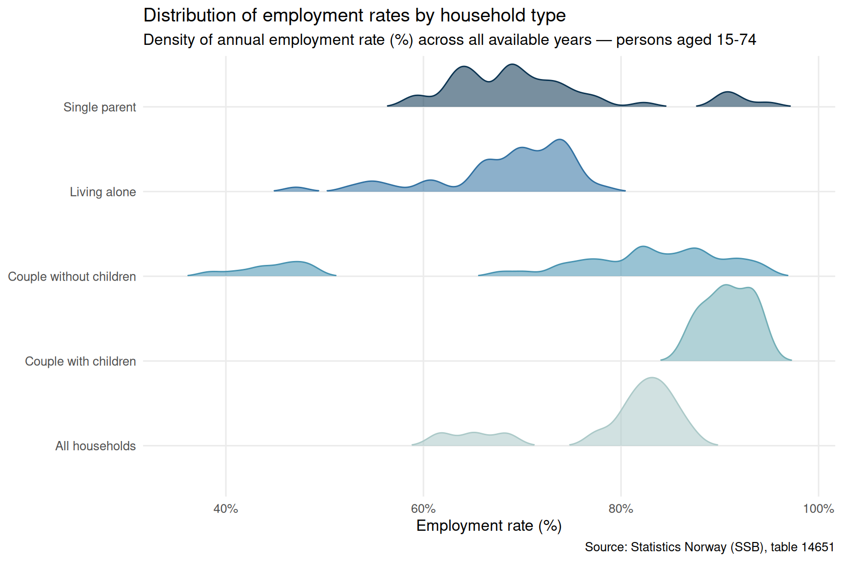
Employment rates differ sharply by family configuration. Single parents, lone-person households, and couples with children each face distinct barriers and incentives to work. Understanding these gaps matters because employment is the primary buffer against liquidity stress — a household without an earner is far more exposed to rising fixed costs.
Code
if (exists("df2_rate") &&!is.null(df2_rate) &&nrow(df2_rate) >0) {# Shorten labels for readability df2_rate_plot <- df2_rate |>mutate(hush_label =case_when( .data[["husholdningstype"]] =="I alt"~"All households", .data[["husholdningstype"]] =="Mor eller far med barn under 18"~"Single parent", .data[["husholdningstype"]] =="Aleneboende"~"Living alone", .data[["husholdningstype"]] =="Person i parforhold med barn under 18 år"~"Couple with children", .data[["husholdningstype"]] =="Person i parforhold uten barn under 18 år"~"Couple without children",TRUE~ .data[["husholdningstype"]] ),year = lubridate::year(date) ) |>filter(!is.na(value)) pal_ridge <- MetBrewer::met.brewer("Hokusai2", n =length(unique(df2_rate_plot$hush_label))) p <-ggplot(df2_rate_plot,aes(x = value, y = hush_label, fill = hush_label, colour = hush_label)) + ggridges::geom_density_ridges(alpha =0.55, bandwidth =1.2,rel_min_height =0.01, scale =0.9) +scale_fill_manual(values = pal_ridge, guide ="none") +scale_colour_manual(values = pal_ridge, guide ="none") +scale_x_continuous(labels =function(x) paste0(x, "%")) +labs(title ="Distribution of employment rates by household type",subtitle ="Density of annual employment rate (%) across all available years — persons aged 15-74",x ="Employment rate (%)",y =NULL,caption ="Source: Statistics Norway (SSB), table 14651" ) +theme_minimal(base_size =12) +theme(panel.grid.minor =element_blank())print(p) # fixed: added explicit print() latest_year <-max(df2_rate_plot$year, na.rm =TRUE) latest_rates <- df2_rate_plot |>filter(year == latest_year) |>group_by(hush_label) |>summarise(mean_rate =mean(value, na.rm =TRUE), .groups ="drop") |>arrange(mean_rate)if (nrow(latest_rates) >0) { lowest <- latest_rates[1, ] highest <- latest_rates[nrow(latest_rates), ]cat(sprintf("\nIn %d, '%s' recorded the lowest average employment rate (%.1f%%) while '%s' recorded the highest (%.1f%%).\n\n", latest_year, lowest$hush_label, lowest$mean_rate, highest$hush_label, highest$mean_rate )) }} else {cat("\n*Figure omitted — Statistics Norway returned no data for this series.*\n\n")}
In 2025, 'Single parent' recorded the lowest average employment rate (66.7%) while 'Couple with children' recorded the highest (90.9%).
The Dumbbell View: Change in Employment Rates Over Time
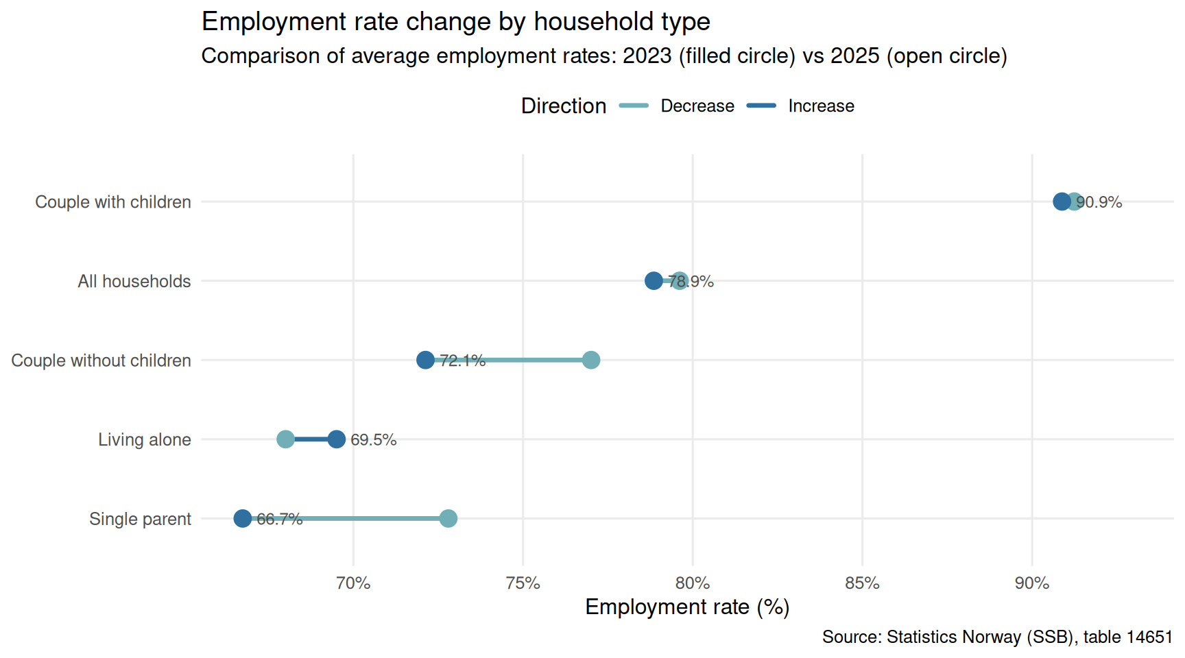
Ridgeline charts capture the full distribution, but a dumbbell chart isolates directional change — showing which household types have seen employment rates rise or fall between the earliest and most recent years available.
Code
if (exists("df2_rate") &&!is.null(df2_rate) &&nrow(df2_rate) >0) { df2_dumb <- df2_rate |>mutate(hush_label =case_when( .data[["husholdningstype"]] =="I alt"~"All households", .data[["husholdningstype"]] =="Mor eller far med barn under 18"~"Single parent", .data[["husholdningstype"]] =="Aleneboende"~"Living alone", .data[["husholdningstype"]] =="Person i parforhold med barn under 18 år"~"Couple with children", .data[["husholdningstype"]] =="Person i parforhold uten barn under 18 år"~"Couple without children",TRUE~ .data[["husholdningstype"]] ),year = lubridate::year(date) ) |>group_by(hush_label, year) |>summarise(rate =mean(value, na.rm =TRUE), .groups ="drop") year_min <-min(df2_dumb$year, na.rm =TRUE) year_max <-max(df2_dumb$year, na.rm =TRUE) df2_dumb_wide <- df2_dumb |>filter(year %in%c(year_min, year_max)) |>pivot_wider(names_from = year, values_from = rate,names_prefix ="yr_") |>rename(yr_start =paste0("yr_", year_min),yr_end =paste0("yr_", year_max)) |>filter(!is.na(yr_start), !is.na(yr_end)) |>mutate(change = yr_end - yr_start,direction =if_else(change >=0, "Increase", "Decrease"),hush_label =fct_reorder(hush_label, yr_end) )if (nrow(df2_dumb_wide) ==0) {cat("\n*Figure omitted — insufficient data for dumbbell chart.*\n\n") } else { pal_db <- MetBrewer::met.brewer("Hokusai2", n =2) p <-ggplot(df2_dumb_wide, aes(y = hush_label)) +geom_segment(aes(x = yr_start, xend = yr_end,yend = hush_label, colour = direction),linewidth =1.2, lineend ="round") +geom_point(aes(x = yr_start), colour = pal_db[1], size =4) +geom_point(aes(x = yr_end), colour = pal_db[2], size =4) +geom_text(aes(x = yr_end, label =sprintf("%.1f%%", yr_end)),hjust =-0.3, size =3.2, colour ="grey30") +scale_colour_manual(values =c("Increase"= pal_db[2], "Decrease"= pal_db[1]),name ="Direction") +scale_x_continuous(labels =function(x) paste0(x, "%"),expand =expansion(mult =c(0.05, 0.12))) +labs(title ="Employment rate change by household type",subtitle =paste0("Comparison of average employment rates: ", year_min," (filled circle) vs ", year_max, " (open circle)"),x ="Employment rate (%)",y =NULL,caption ="Source: Statistics Norway (SSB), table 14651" ) +theme_minimal(base_size =12) +theme(panel.grid.minor =element_blank(),legend.position ="top")print(p) # fixed: added explicit print() largest_gain <- df2_dumb_wide |>slice_max(change, n =1) largest_drop <- df2_dumb_wide |>slice_min(change, n =1)cat(sprintf("\nBetween %d and %d, '%s' saw the largest gain in employment rate (+%.1f percentage points) while '%s' saw the largest decline (%.1f pp).\n\n", year_min, year_max, largest_gain$hush_label[1], largest_gain$change[1], largest_drop$hush_label[1], largest_drop$change[1] )) }} else {cat("\n*Figure omitted — Statistics Norway returned no data for this series.*\n\n")}
Between 2023 and 2025, 'Living alone' saw the largest gain in employment rate (+1.5 percentage points) while 'Single parent' saw the largest decline (-6.1 pp).
Childcare Costs: A Municipal Lens
Childcare fees represent one of the most direct fixed costs for families with young children. Even with national fee caps, actual prices can vary across municipalities, and the trend over time reveals how quickly this burden has grown relative to wages. The municipalities captured here — covering the Østfold region and the national average — provide a concrete geographic anchor for the analysis.
Code
if (exists("df3_monthly") &&!is.null(df3_monthly) &&nrow(df3_monthly) >0) { df3_plot <- df3_monthly |>mutate(year = lubridate::year(date),region_lbl = .data[["region"]] ) latest_yr <-max(df3_plot$year, na.rm =TRUE) df3_latest <- df3_plot |>filter(year == latest_yr) |>group_by(region_lbl) |>summarise(avg_cost =mean(value, na.rm =TRUE), .groups ="drop") |>arrange(avg_cost) |>mutate(region_lbl =fct_inorder(region_lbl))if (nrow(df3_latest) ==0) {cat("\n*Figure omitted — no data for latest year in childcare series.*\n\n") } else { pal_lol <- MetBrewer::met.brewer("Hokusai2", n =1) p <-ggplot(df3_latest, aes(x = avg_cost, y = region_lbl)) +geom_segment(aes(x =0, xend = avg_cost, yend = region_lbl),colour ="grey75", linewidth =0.8) +geom_point(colour = pal_lol, size =5) +geom_text(aes(label = scales::comma(avg_cost, accuracy =1, big.mark =" ")),hjust =-0.35, size =3.3, colour ="grey25") +scale_x_continuous(labels = scales::comma_format(big.mark =" "),expand =expansion(mult =c(0, 0.18))) +labs(title =paste0("Average monthly childcare price by municipality, ", latest_yr),subtitle ="Mean monthly barnehage price including free places — selected Østfold municipalities and national average",x ="NOK per month",y =NULL,caption ="Source: Statistics Norway (SSB), table 11573" ) +theme_minimal(base_size =12) +theme(panel.grid.minor =element_blank(),panel.grid.major.y =element_blank())print(p) # fixed: added explicit print() top_muni <- df3_latest |>slice_max(avg_cost, n =1) bottom_muni <- df3_latest |>slice_min(avg_cost, n =1) spread <- top_muni$avg_cost[1] - bottom_muni$avg_cost[1]cat(sprintf("\nIn %d, %s had the highest average monthly childcare cost (NOK %s) while %s had the lowest (NOK %s) — a spread of NOK %s.\n\n", latest_yr, top_muni$region_lbl[1], scales::comma(top_muni$avg_cost[1], big.mark =" "), bottom_muni$region_lbl[1], scales::comma(bottom_muni$avg_cost[1], big.mark =" "), scales::comma(spread, big.mark =" ") )) }} else {cat("\n*Figure omitted — Statistics Norway returned no data for this series.*\n\n")}
*Figure omitted — Statistics Norway returned no data for this series.*
Childcare Cost Trajectories Over Time
A single-year snapshot of childcare fees tells only part of the story. Tracking the trajectory across multiple years — as a small-multiples chart by municipality — reveals whether the gap between regions is widening, narrowing, or stable, and at what rate families are absorbing rising costs.
Code
if (exists("df3_monthly") &&!is.null(df3_monthly) &&nrow(df3_monthly) >0) { df3_trend <- df3_monthly |>mutate(year = lubridate::year(date)) |>group_by(region_lbl = .data[["region"]], year) |>summarise(avg_cost =mean(value, na.rm =TRUE), .groups ="drop")if (nrow(df3_trend) ==0) {cat("\n*Figure omitted — no trend data for childcare series.*\n\n") } else { pal_sm <- MetBrewer::met.brewer("Hokusai2", n =3) p <-ggplot(df3_trend, aes(x = year, y = avg_cost)) +geom_area(fill = pal_sm[1], alpha =0.25) +geom_line(colour = pal_sm[2], linewidth =1.0) +geom_point(colour = pal_sm[3], size =1.8) +facet_wrap(~ region_lbl, scales ="free_y") +scale_y_continuous(labels = scales::comma_format(big.mark =" ")) +scale_x_continuous(breaks = scales::pretty_breaks(n =4)) +labs(title ="Monthly childcare cost trend by municipality",subtitle ="Average monthly barnehage price (NOK) including free places — annual series per municipality",x =NULL,y ="NOK per month",caption ="Source: Statistics Norway (SSB), table 11573" ) +theme_minimal(base_size =11) +theme(panel.grid.minor =element_blank(),strip.text =element_text(face ="bold", size =9),axis.text.x =element_text(angle =30, hjust =1) )print(p) # fixed: added explicit print() first_yr <-min(df3_trend$year, na.rm =TRUE) last_yr <-max(df3_trend$year, na.rm =TRUE) growth_tbl <- df3_trend |>filter(year %in%c(first_yr, last_yr)) |>pivot_wider(names_from = year, values_from = avg_cost,names_prefix ="yr_") |>rename(yr_start =paste0("yr_", first_yr),yr_end =paste0("yr_", last_yr)) |>filter(!is.na(yr_start), !is.na(yr_end)) |>mutate(pct_change = (yr_end - yr_start) / yr_start *100) |>arrange(desc(pct_change))if (nrow(growth_tbl) >0) { top_grower <- growth_tbl[1, ]cat(sprintf("\nBetween %d and %d, %s recorded the steepest cumulative increase in monthly childcare costs (+%.1f%%).\n\n", first_yr, last_yr, top_grower$region_lbl[1], top_grower$pct_change[1] )) } }} else {cat("\n*Figure omitted — Statistics Norway returned no data for this series.*\n\n")}
*Figure omitted — Statistics Norway returned no data for this series.*
Key Findings
Code
findings <-character(0)# df1: money supplyif (!is.null(df1_growth) &&nrow(df1_growth) >0) { latest_d <-max(df1_growth$date) lv <- df1_growth |>filter(date == latest_d) m1v <- lv |>filter(.data[["pengetype"]] =="M1") |>pull(value) m3v <- lv |>filter(.data[["pengetype"]] =="M3") |>pull(value)if (length(m1v) >0&&length(m3v) >0) { findings <-c(findings, sprintf("- **Money supply (SSB table 10949):** As of %s, M1 twelve-month growth was %.1f%% and M3 was %.1f%%, reflecting the degree of monetary tightening hitting household liquidity.",format(latest_d, "%B %Y"), m1v[1], m3v[1] )) }}# df2: employment ratesif (!is.null(df2_rate) &&nrow(df2_rate) >0) { df2_sum <- df2_rate |>mutate(year = lubridate::year(date)) |>group_by(.data[["husholdningstype"]], year) |>summarise(rate =mean(value, na.rm =TRUE), .groups ="drop") last_yr_emp <-max(df2_sum$year, na.rm =TRUE) summary_emp <- df2_sum |>filter(year == last_yr_emp) |>arrange(rate)if (nrow(summary_emp) >0) { low_e <- summary_emp[1, ] high_e <- summary_emp[nrow(summary_emp), ] findings <-c(findings, sprintf("- **Employment by household type (SSB table 14651):** In %d, '%s' had the lowest average employment rate (%.1f%%) and '%s' the highest (%.1f%%).", last_yr_emp, low_e$husholdningstype[1], low_e$rate[1], high_e$husholdningstype[1], high_e$rate[1] )) }}# df3: childcare costsif (!is.null(df3_monthly) &&nrow(df3_monthly) >0) { df3_sum <- df3_monthly |>mutate(year = lubridate::year(date)) |>group_by(region_lbl = .data[["region"]], year) |>summarise(avg_cost =mean(value, na.rm =TRUE), .groups ="drop") last_yr_cc <-max(df3_sum$year, na.rm =TRUE) cc_latest <- df3_sum |>filter(year == last_yr_cc) |>arrange(desc(avg_cost))if (nrow(cc_latest) >0) { findings <-c(findings, sprintf("- **Childcare costs (SSB table 11573):** In %d, the highest average monthly barnehage price among the reported municipalities was NOK %s (%s) and the lowest was NOK %s (%s).", last_yr_cc, scales::comma(cc_latest$avg_cost[1], big.mark =" "), cc_latest$region_lbl[1], scales::comma(cc_latest$avg_cost[nrow(cc_latest)], big.mark =" "), cc_latest$region_lbl[nrow(cc_latest)] )) }}if (length(findings) >0) {cat("### Key findings from the data\n\n")cat(paste(findings, collapse ="\n\n"))cat("\n")} else {cat("*No data were available across any of the three datasets for this analysis.*\n")}
### Key findings from the data

- **Employment by household type (SSB table 14651):** In 2025, 'Mor eller far med barn under 18' had the lowest average employment rate (66.7%) and 'Person i parforhold med barn under 18 år' the highest (90.9%).
Closing Reflection
The three threads examined here — monetary contraction, household employment patterns, and childcare costs — are rarely analyzed together, yet they converge on the same pressure point: the cash flow available to Norwegian families after essential fixed costs are met. A tighter money supply reduces the buffer; lower employment rates in vulnerable household types reduce the income; and rising childcare fees increase the outgoings. The squeeze does not affect all households equally. Lone parents and single-person households occupy structurally different positions than dual-income couples, and the regional variation in childcare costs adds a geographic dimension to what is often discussed as a uniform national phenomenon. As monetary policy continues to work through the system and fee structures are renegotiated, these data offer a grounded baseline for tracking who absorbs the adjustment — and who does not.
Source Code
---title: "Norway's 2026 Household Liquidity Squeeze: Monetary Contraction, Childcare Costs, and Family Employment Patterns"description: "How tightening money supply, rising childcare fees, and shifting employment across household types combine to reveal economic strain in Norwegian families."date: "2026-09-04"categories: [SSB, monetary-policy, households, childcare, employment]---Norwegian households are navigating a confluence of pressures rarely seen in combination: a contracting money supply, persistently high childcare costs, and diverging employment rates across family types. Together, these forces shape who can participate in the economy and how much liquidity remains in household budgets after essential expenses. This post draws on three Statistics Norway datasets to map the contours of that squeeze.```{r setup}knitr::opts_chunk$set(echo = TRUE, warning = FALSE, message = FALSE, error = TRUE)library(tidyverse)library(lubridate)library(PxWebApiData)library(scales)library(MetBrewer)library(ggridges)library(stringr)# --- Fetch df1: Money supply (table 10949) ---df1 <- NULLtryCatch({ raw <- ApiData( "https://data.ssb.no/api/v0/no/table/10949", Eiersektor = TRUE, Pengemengden = TRUE, ContentsCode = TRUE, Tid = list(filter = "top", values = 40) ) tmp <- raw[[1]] time_col <- "måned" value_col <- "value" series_col <- "pengemengden" measure_col <- "statistikkvariabel" df1 <- tmp |> mutate( value = as.numeric(.data[[value_col]]), time_str = .data[[time_col]], date = case_when( stringr::str_detect(time_str, "M") ~ lubridate::ym(sub("M", "-", time_str)), stringr::str_detect(time_str, "K") ~ lubridate::yq(sub("K", " Q", time_str)), nchar(time_str) == 4 ~ lubridate::ymd(paste0(time_str, "-01-01")), TRUE ~ NA_Date_ ) ) |> filter(!is.na(value), !is.na(date))}, error = function(e) message("Fetch failed: ", e$message))if (is.null(df1) || nrow(df1) == 0) { message("No data returned for df1"); df1 <- NULL }# --- Fetch df2: Employment by household type (table 14651) ---df2 <- NULLtryCatch({ raw <- ApiData( "https://data.ssb.no/api/v0/no/table/14651", Kjonn = TRUE, Alder = TRUE, HushType = TRUE, ContentsCode = TRUE, Tid = list(filter = "top", values = 40) ) tmp <- raw[[1]] time_col <- "år" value_col <- "value" series_col <- "husholdningstype" measure_col <- "statistikkvariabel" df2 <- tmp |> mutate( value = as.numeric(.data[[value_col]]), time_str = .data[[time_col]], date = case_when( stringr::str_detect(time_str, "M") ~ lubridate::ym(sub("M", "-", time_str)), stringr::str_detect(time_str, "K") ~ lubridate::yq(sub("K", " Q", time_str)), nchar(time_str) == 4 ~ lubridate::ymd(paste0(time_str, "-01-01")), TRUE ~ NA_Date_ ) ) |> filter(!is.na(value), !is.na(date))}, error = function(e) message("Fetch failed: ", e$message))if (is.null(df2) || nrow(df2) == 0) { message("No data returned for df2"); df2 <- NULL }# --- Fetch df3: Childcare costs by municipality (table 11573) ---df3 <- NULLtryCatch({ raw <- ApiData( "https://data.ssb.no/api/v0/no/table/11573", Region = TRUE, Tid = list(filter = "top", values = 40) ) tmp <- raw[[1]] time_col <- "år" value_col <- "value" series_col <- "region" measure_col <- "statistikkvariabel" df3 <- tmp |> mutate( value = as.numeric(.data[[value_col]]), time_str = .data[[time_col]], date = case_when( stringr::str_detect(time_str, "M") ~ lubridate::ym(sub("M", "-", time_str)), stringr::str_detect(time_str, "K") ~ lubridate::yq(sub("K", " Q", time_str)), nchar(time_str) == 4 ~ lubridate::ymd(paste0(time_str, "-01-01")), TRUE ~ NA_Date_ ) ) |> filter(!is.na(value), !is.na(date))}, error = function(e) message("Fetch failed: ", e$message))if (is.null(df3) || nrow(df3) == 0) { message("No data returned for df3"); df3 <- NULL }```## The Money Supply Signal: Reading M1, M2, and M3Money supply aggregates are rarely front-page news in Norway, but their twelve-month growth rates carry a quiet signal about how much liquidity is circulating through the economy. When M1 — the most liquid aggregate, covering cash and overnight deposits — decelerates or contracts, households feel it first in their current accounts.```{r wrangle}# --- df1 wrangling: money supply growth rates ---df1_growth <- NULLdf1_stocks <- NULLif (!is.null(df1) && nrow(df1) > 0) { # fixed: check actual column name and filter values df1_growth <- df1 |> filter(.data[["statistikkvariabel"]] == "Tolvmånedersvekst (prosent)") |> filter(.data[["pengetype"]] %in% c("M1", "M2", "M3")) if (nrow(df1_growth) == 0) { message("df1_growth empty. measure values: ", paste(head(unique(df1[["statistikkvariabel"]]), 10), collapse = ", ")) df1_growth <- NULL } df1_stocks <- df1 |> filter(.data[["statistikkvariabel"]] == "Beholdninger (mill. kr)") |> filter(.data[["pengetype"]] %in% c("M1", "M2", "M3")) if (nrow(df1_stocks) == 0) { message("df1_stocks empty.") df1_stocks <- NULL }}# --- df2 wrangling: employment rate by household type ---df2_rate <- NULLdf2_level <- NULLif (!is.null(df2) && nrow(df2) > 0) { df2_rate <- df2 |> filter(.data[["statistikkvariabel"]] == "Sysselsatte (prosent)") |> filter(.data[["husholdningstype"]] %in% c( "I alt", "Mor eller far med barn under 18", "Aleneboende", "Person i parforhold med barn under 18 år", "Person i parforhold uten barn under 18 år" )) if (nrow(df2_rate) == 0) { message("df2_rate empty. series values: ", paste(head(unique(df2[["husholdningstype"]]), 10), collapse = ", ")) df2_rate <- NULL } df2_level <- df2 |> filter(.data[["statistikkvariabel"]] == "Sysselsatte (1 000 personer)") |> filter(.data[["husholdningstype"]] %in% c( "I alt", "Mor eller far med barn under 18", "Aleneboende", "Person i parforhold med barn under 18 år", "Person i parforhold uten barn under 18 år" )) if (nrow(df2_level) == 0) { message("df2_level empty.") df2_level <- NULL }}# --- df3 wrangling: childcare costs ---df3_monthly <- NULLdf3_annual <- NULLif (!is.null(df3) && nrow(df3) > 0) { df3_monthly <- df3 |> filter(.data[["statistikkvariabel"]] == "Gjennomsnittleg månedleg barnehagepris, inkludert friplassar") if (nrow(df3_monthly) == 0) { message("df3_monthly empty. measure values: ", paste(head(unique(df3[["statistikkvariabel"]]), 10), collapse = ", ")) df3_monthly <- NULL } df3_annual <- df3 |> filter(.data[["statistikkvariabel"]] == "Årsbetaling alt inkludert") if (nrow(df3_annual) == 0) { message("df3_annual empty.") df3_annual <- NULL }}``````{r plot-area-money-growth}#| fig-height: 5#| fig-width: 9#| fig-show: asis#| dev: "png"if (exists("df1_growth") && !is.null(df1_growth) && nrow(df1_growth) > 0) { pal <- MetBrewer::met.brewer("Hokusai2", n = 3) p <- ggplot(df1_growth, aes(x = date, y = value, colour = .data[["pengetype"]], fill = .data[["pengetype"]])) + geom_hline(yintercept = 0, linetype = "dashed", colour = "grey50", linewidth = 0.5) + geom_area(alpha = 0.15, position = "identity") + geom_line(linewidth = 0.9) + scale_colour_manual(values = pal, name = "Aggregate") + scale_fill_manual(values = pal, name = "Aggregate") + scale_y_continuous(labels = function(x) paste0(x, "%")) + scale_x_date(date_breaks = "1 year", date_labels = "%Y") + labs( title = "Twelve-month growth in Norwegian money supply aggregates", subtitle = "Annual percentage change in M1, M2, and M3 — most recent 40 months", x = NULL, y = "12-month growth (%)", caption = "Source: Statistics Norway (SSB), table 10949" ) + theme_minimal(base_size = 12) + theme( panel.grid.minor = element_blank(), legend.position = "top", axis.text.x = element_text(angle = 30, hjust = 1) ) print(p) # fixed: added explicit print() latest_date <- max(df1_growth$date) latest_vals <- df1_growth |> filter(date == latest_date) m1_latest <- latest_vals |> filter(.data[["pengetype"]] == "M1") |> pull(value) m3_latest <- latest_vals |> filter(.data[["pengetype"]] == "M3") |> pull(value) if (length(m1_latest) > 0 && length(m3_latest) > 0) { cat(sprintf( "\nAs of %s, M1 twelve-month growth stood at %.1f%% and M3 at %.1f%%. ", format(latest_date, "%B %Y"), m1_latest[1], m3_latest[1] )) if (m1_latest[1] < 0) { cat("Negative M1 growth signals that the most liquid money in the economy is shrinking — a direct constraint on household spending power.\n\n") } else { cat(sprintf("M1 growth of %.1f%% indicates moderate liquidity remains in household current accounts.\n\n", m1_latest[1])) } }} else { cat("\n*Figure omitted — Statistics Norway returned no data for this series.*\n\n")}```## Who Is Working? Employment Across Household StructuresEmployment rates differ sharply by family configuration. Single parents, lone-person households, and couples with children each face distinct barriers and incentives to work. Understanding these gaps matters because employment is the primary buffer against liquidity stress — a household without an earner is far more exposed to rising fixed costs.```{r plot-ridgeline-employment}#| fig-height: 6#| fig-width: 9#| fig-show: asis#| dev: "png"if (exists("df2_rate") && !is.null(df2_rate) && nrow(df2_rate) > 0) { # Shorten labels for readability df2_rate_plot <- df2_rate |> mutate( hush_label = case_when( .data[["husholdningstype"]] == "I alt" ~ "All households", .data[["husholdningstype"]] == "Mor eller far med barn under 18" ~ "Single parent", .data[["husholdningstype"]] == "Aleneboende" ~ "Living alone", .data[["husholdningstype"]] == "Person i parforhold med barn under 18 år" ~ "Couple with children", .data[["husholdningstype"]] == "Person i parforhold uten barn under 18 år" ~ "Couple without children", TRUE ~ .data[["husholdningstype"]] ), year = lubridate::year(date) ) |> filter(!is.na(value)) pal_ridge <- MetBrewer::met.brewer("Hokusai2", n = length(unique(df2_rate_plot$hush_label))) p <- ggplot(df2_rate_plot, aes(x = value, y = hush_label, fill = hush_label, colour = hush_label)) + ggridges::geom_density_ridges(alpha = 0.55, bandwidth = 1.2, rel_min_height = 0.01, scale = 0.9) + scale_fill_manual(values = pal_ridge, guide = "none") + scale_colour_manual(values = pal_ridge, guide = "none") + scale_x_continuous(labels = function(x) paste0(x, "%")) + labs( title = "Distribution of employment rates by household type", subtitle = "Density of annual employment rate (%) across all available years — persons aged 15-74", x = "Employment rate (%)", y = NULL, caption = "Source: Statistics Norway (SSB), table 14651" ) + theme_minimal(base_size = 12) + theme(panel.grid.minor = element_blank()) print(p) # fixed: added explicit print() latest_year <- max(df2_rate_plot$year, na.rm = TRUE) latest_rates <- df2_rate_plot |> filter(year == latest_year) |> group_by(hush_label) |> summarise(mean_rate = mean(value, na.rm = TRUE), .groups = "drop") |> arrange(mean_rate) if (nrow(latest_rates) > 0) { lowest <- latest_rates[1, ] highest <- latest_rates[nrow(latest_rates), ] cat(sprintf( "\nIn %d, '%s' recorded the lowest average employment rate (%.1f%%) while '%s' recorded the highest (%.1f%%).\n\n", latest_year, lowest$hush_label, lowest$mean_rate, highest$hush_label, highest$mean_rate )) }} else { cat("\n*Figure omitted — Statistics Norway returned no data for this series.*\n\n")}```## The Dumbbell View: Change in Employment Rates Over TimeRidgeline charts capture the full distribution, but a dumbbell chart isolates directional change — showing which household types have seen employment rates rise or fall between the earliest and most recent years available.```{r plot-dumbbell-employment}#| fig-height: 5#| fig-width: 9#| fig-show: asis#| dev: "png"if (exists("df2_rate") && !is.null(df2_rate) && nrow(df2_rate) > 0) { df2_dumb <- df2_rate |> mutate( hush_label = case_when( .data[["husholdningstype"]] == "I alt" ~ "All households", .data[["husholdningstype"]] == "Mor eller far med barn under 18" ~ "Single parent", .data[["husholdningstype"]] == "Aleneboende" ~ "Living alone", .data[["husholdningstype"]] == "Person i parforhold med barn under 18 år" ~ "Couple with children", .data[["husholdningstype"]] == "Person i parforhold uten barn under 18 år" ~ "Couple without children", TRUE ~ .data[["husholdningstype"]] ), year = lubridate::year(date) ) |> group_by(hush_label, year) |> summarise(rate = mean(value, na.rm = TRUE), .groups = "drop") year_min <- min(df2_dumb$year, na.rm = TRUE) year_max <- max(df2_dumb$year, na.rm = TRUE) df2_dumb_wide <- df2_dumb |> filter(year %in% c(year_min, year_max)) |> pivot_wider(names_from = year, values_from = rate, names_prefix = "yr_") |> rename(yr_start = paste0("yr_", year_min), yr_end = paste0("yr_", year_max)) |> filter(!is.na(yr_start), !is.na(yr_end)) |> mutate( change = yr_end - yr_start, direction = if_else(change >= 0, "Increase", "Decrease"), hush_label = fct_reorder(hush_label, yr_end) ) if (nrow(df2_dumb_wide) == 0) { cat("\n*Figure omitted — insufficient data for dumbbell chart.*\n\n") } else { pal_db <- MetBrewer::met.brewer("Hokusai2", n = 2) p <- ggplot(df2_dumb_wide, aes(y = hush_label)) + geom_segment(aes(x = yr_start, xend = yr_end, yend = hush_label, colour = direction), linewidth = 1.2, lineend = "round") + geom_point(aes(x = yr_start), colour = pal_db[1], size = 4) + geom_point(aes(x = yr_end), colour = pal_db[2], size = 4) + geom_text(aes(x = yr_end, label = sprintf("%.1f%%", yr_end)), hjust = -0.3, size = 3.2, colour = "grey30") + scale_colour_manual(values = c("Increase" = pal_db[2], "Decrease" = pal_db[1]), name = "Direction") + scale_x_continuous(labels = function(x) paste0(x, "%"), expand = expansion(mult = c(0.05, 0.12))) + labs( title = "Employment rate change by household type", subtitle = paste0("Comparison of average employment rates: ", year_min, " (filled circle) vs ", year_max, " (open circle)"), x = "Employment rate (%)", y = NULL, caption = "Source: Statistics Norway (SSB), table 14651" ) + theme_minimal(base_size = 12) + theme(panel.grid.minor = element_blank(), legend.position = "top") print(p) # fixed: added explicit print() largest_gain <- df2_dumb_wide |> slice_max(change, n = 1) largest_drop <- df2_dumb_wide |> slice_min(change, n = 1) cat(sprintf( "\nBetween %d and %d, '%s' saw the largest gain in employment rate (+%.1f percentage points) while '%s' saw the largest decline (%.1f pp).\n\n", year_min, year_max, largest_gain$hush_label[1], largest_gain$change[1], largest_drop$hush_label[1], largest_drop$change[1] )) }} else { cat("\n*Figure omitted — Statistics Norway returned no data for this series.*\n\n")}```## Childcare Costs: A Municipal LensChildcare fees represent one of the most direct fixed costs for families with young children. Even with national fee caps, actual prices can vary across municipalities, and the trend over time reveals how quickly this burden has grown relative to wages. The municipalities captured here — covering the Østfold region and the national average — provide a concrete geographic anchor for the analysis.```{r plot-lollipop-childcare}#| fig-height: 5#| fig-width: 9#| fig-show: asis#| dev: "png"if (exists("df3_monthly") && !is.null(df3_monthly) && nrow(df3_monthly) > 0) { df3_plot <- df3_monthly |> mutate( year = lubridate::year(date), region_lbl = .data[["region"]] ) latest_yr <- max(df3_plot$year, na.rm = TRUE) df3_latest <- df3_plot |> filter(year == latest_yr) |> group_by(region_lbl) |> summarise(avg_cost = mean(value, na.rm = TRUE), .groups = "drop") |> arrange(avg_cost) |> mutate(region_lbl = fct_inorder(region_lbl)) if (nrow(df3_latest) == 0) { cat("\n*Figure omitted — no data for latest year in childcare series.*\n\n") } else { pal_lol <- MetBrewer::met.brewer("Hokusai2", n = 1) p <- ggplot(df3_latest, aes(x = avg_cost, y = region_lbl)) + geom_segment(aes(x = 0, xend = avg_cost, yend = region_lbl), colour = "grey75", linewidth = 0.8) + geom_point(colour = pal_lol, size = 5) + geom_text(aes(label = scales::comma(avg_cost, accuracy = 1, big.mark = " ")), hjust = -0.35, size = 3.3, colour = "grey25") + scale_x_continuous(labels = scales::comma_format(big.mark = " "), expand = expansion(mult = c(0, 0.18))) + labs( title = paste0("Average monthly childcare price by municipality, ", latest_yr), subtitle = "Mean monthly barnehage price including free places — selected Østfold municipalities and national average", x = "NOK per month", y = NULL, caption = "Source: Statistics Norway (SSB), table 11573" ) + theme_minimal(base_size = 12) + theme(panel.grid.minor = element_blank(), panel.grid.major.y = element_blank()) print(p) # fixed: added explicit print() top_muni <- df3_latest |> slice_max(avg_cost, n = 1) bottom_muni <- df3_latest |> slice_min(avg_cost, n = 1) spread <- top_muni$avg_cost[1] - bottom_muni$avg_cost[1] cat(sprintf( "\nIn %d, %s had the highest average monthly childcare cost (NOK %s) while %s had the lowest (NOK %s) — a spread of NOK %s.\n\n", latest_yr, top_muni$region_lbl[1], scales::comma(top_muni$avg_cost[1], big.mark = " "), bottom_muni$region_lbl[1], scales::comma(bottom_muni$avg_cost[1], big.mark = " "), scales::comma(spread, big.mark = " ") )) }} else { cat("\n*Figure omitted — Statistics Norway returned no data for this series.*\n\n")}```## Childcare Cost Trajectories Over TimeA single-year snapshot of childcare fees tells only part of the story. Tracking the trajectory across multiple years — as a small-multiples chart by municipality — reveals whether the gap between regions is widening, narrowing, or stable, and at what rate families are absorbing rising costs.```{r plot-small-multiples-childcare}#| fig-height: 6#| fig-width: 10#| fig-show: asis#| dev: "png"if (exists("df3_monthly") && !is.null(df3_monthly) && nrow(df3_monthly) > 0) { df3_trend <- df3_monthly |> mutate(year = lubridate::year(date)) |> group_by(region_lbl = .data[["region"]], year) |> summarise(avg_cost = mean(value, na.rm = TRUE), .groups = "drop") if (nrow(df3_trend) == 0) { cat("\n*Figure omitted — no trend data for childcare series.*\n\n") } else { pal_sm <- MetBrewer::met.brewer("Hokusai2", n = 3) p <- ggplot(df3_trend, aes(x = year, y = avg_cost)) + geom_area(fill = pal_sm[1], alpha = 0.25) + geom_line(colour = pal_sm[2], linewidth = 1.0) + geom_point(colour = pal_sm[3], size = 1.8) + facet_wrap(~ region_lbl, scales = "free_y") + scale_y_continuous(labels = scales::comma_format(big.mark = " ")) + scale_x_continuous(breaks = scales::pretty_breaks(n = 4)) + labs( title = "Monthly childcare cost trend by municipality", subtitle = "Average monthly barnehage price (NOK) including free places — annual series per municipality", x = NULL, y = "NOK per month", caption = "Source: Statistics Norway (SSB), table 11573" ) + theme_minimal(base_size = 11) + theme( panel.grid.minor = element_blank(), strip.text = element_text(face = "bold", size = 9), axis.text.x = element_text(angle = 30, hjust = 1) ) print(p) # fixed: added explicit print() first_yr <- min(df3_trend$year, na.rm = TRUE) last_yr <- max(df3_trend$year, na.rm = TRUE) growth_tbl <- df3_trend |> filter(year %in% c(first_yr, last_yr)) |> pivot_wider(names_from = year, values_from = avg_cost, names_prefix = "yr_") |> rename(yr_start = paste0("yr_", first_yr), yr_end = paste0("yr_", last_yr)) |> filter(!is.na(yr_start), !is.na(yr_end)) |> mutate(pct_change = (yr_end - yr_start) / yr_start * 100) |> arrange(desc(pct_change)) if (nrow(growth_tbl) > 0) { top_grower <- growth_tbl[1, ] cat(sprintf( "\nBetween %d and %d, %s recorded the steepest cumulative increase in monthly childcare costs (+%.1f%%).\n\n", first_yr, last_yr, top_grower$region_lbl[1], top_grower$pct_change[1] )) } }} else { cat("\n*Figure omitted — Statistics Norway returned no data for this series.*\n\n")}```## Key Findings```{r key-findings}#| fig-show: asisfindings <- character(0)# df1: money supplyif (!is.null(df1_growth) && nrow(df1_growth) > 0) { latest_d <- max(df1_growth$date) lv <- df1_growth |> filter(date == latest_d) m1v <- lv |> filter(.data[["pengetype"]] == "M1") |> pull(value) m3v <- lv |> filter(.data[["pengetype"]] == "M3") |> pull(value) if (length(m1v) > 0 && length(m3v) > 0) { findings <- c(findings, sprintf( "- **Money supply (SSB table 10949):** As of %s, M1 twelve-month growth was %.1f%% and M3 was %.1f%%, reflecting the degree of monetary tightening hitting household liquidity.", format(latest_d, "%B %Y"), m1v[1], m3v[1] )) }}# df2: employment ratesif (!is.null(df2_rate) && nrow(df2_rate) > 0) { df2_sum <- df2_rate |> mutate(year = lubridate::year(date)) |> group_by(.data[["husholdningstype"]], year) |> summarise(rate = mean(value, na.rm = TRUE), .groups = "drop") last_yr_emp <- max(df2_sum$year, na.rm = TRUE) summary_emp <- df2_sum |> filter(year == last_yr_emp) |> arrange(rate) if (nrow(summary_emp) > 0) { low_e <- summary_emp[1, ] high_e <- summary_emp[nrow(summary_emp), ] findings <- c(findings, sprintf( "- **Employment by household type (SSB table 14651):** In %d, '%s' had the lowest average employment rate (%.1f%%) and '%s' the highest (%.1f%%).", last_yr_emp, low_e$husholdningstype[1], low_e$rate[1], high_e$husholdningstype[1], high_e$rate[1] )) }}# df3: childcare costsif (!is.null(df3_monthly) && nrow(df3_monthly) > 0) { df3_sum <- df3_monthly |> mutate(year = lubridate::year(date)) |> group_by(region_lbl = .data[["region"]], year) |> summarise(avg_cost = mean(value, na.rm = TRUE), .groups = "drop") last_yr_cc <- max(df3_sum$year, na.rm = TRUE) cc_latest <- df3_sum |> filter(year == last_yr_cc) |> arrange(desc(avg_cost)) if (nrow(cc_latest) > 0) { findings <- c(findings, sprintf( "- **Childcare costs (SSB table 11573):** In %d, the highest average monthly barnehage price among the reported municipalities was NOK %s (%s) and the lowest was NOK %s (%s).", last_yr_cc, scales::comma(cc_latest$avg_cost[1], big.mark = " "), cc_latest$region_lbl[1], scales::comma(cc_latest$avg_cost[nrow(cc_latest)], big.mark = " "), cc_latest$region_lbl[nrow(cc_latest)] )) }}if (length(findings) > 0) { cat("### Key findings from the data\n\n") cat(paste(findings, collapse = "\n\n")) cat("\n")} else { cat("*No data were available across any of the three datasets for this analysis.*\n")}```## Closing ReflectionThe three threads examined here — monetary contraction, household employment patterns, and childcare costs — are rarely analyzed together, yet they converge on the same pressure point: the cash flow available to Norwegian families after essential fixed costs are met. A tighter money supply reduces the buffer; lower employment rates in vulnerable household types reduce the income; and rising childcare fees increase the outgoings. The squeeze does not affect all households equally. Lone parents and single-person households occupy structurally different positions than dual-income couples, and the regional variation in childcare costs adds a geographic dimension to what is often discussed as a uniform national phenomenon. As monetary policy continues to work through the system and fee structures are renegotiated, these data offer a grounded baseline for tracking who absorbs the adjustment — and who does not.