A data-driven investigation into the disconnect between Norway’s household spending patterns, greenhouse gas emissions by source, and regional petroleum product consumption.
Published
September 1, 2026
Norway presents one of the most striking contradictions in modern economics: a country that leads the world in electric vehicle adoption and renewable electricity production yet continues to generate substantial greenhouse gas emissions while its households navigate a turbulent spending environment. This post puts three SSB datasets in conversation — national accounts consumption data, emissions by source, and petroleum product sales — to explore what is actually happening beneath the surface of Norway’s green transition narrative.
Norway’s national accounts reveal a consumption landscape under pressure. Volume changes in household spending — stripped of price effects — tell the most honest story about whether Norwegian families are actually buying more or less. Two components matter most here: goods consumption and services consumption, and their diverging trajectories illuminate the structural forces at play.
Chart 1 — Household Consumption Volume: Goods vs. Services vs. Public Spending
The area chart below tracks quarter-by-quarter volume changes across the three main consumption categories. Positive values mean real spending growth; negative values mean genuine contraction.
Code
if (exists("df1_volume") &&!is.null(df1_volume) &&nrow(df1_volume) >0) { pal <-met.brewer("Hokusai1", n =4) p <-ggplot(df1_volume,aes(x = date, y = value,fill = .data[["makrostørrelse"]],colour = .data[["makrostørrelse"]])) +geom_area(alpha =0.25, position ="identity") +geom_line(linewidth =0.75) +geom_hline(yintercept =0, linetype ="dashed", colour ="grey40", linewidth =0.5) +scale_fill_manual(values = pal, name =NULL) +scale_colour_manual(values = pal, name =NULL) +scale_x_date(date_breaks ="1 year", date_labels ="%Y") +scale_y_continuous(labels =label_number(suffix ="%")) +labs(title ="Norwegian Household and Public Consumption: Volume Change Year-on-Year",subtitle ="Quarterly volume change from same period previous year, by consumption category (percent)",caption ="Source: Statistics Norway, table 09190",x =NULL, y ="Volume change (%)" ) +theme_minimal(base_size =12) +theme(legend.position ="bottom",panel.grid.minor =element_blank(),plot.title =element_text(face ="bold", size =13),plot.subtitle =element_text(colour ="grey40", size =10),plot.caption =element_text(colour ="grey55", size =9) )print(p) # fixed: added explicit print() to ensure figure renders latest_q <- df1_volume |>filter(date ==max(date)) goods_row <- latest_q |>filter(.data[["makrostørrelse"]] =="Varekonsum") serv_row <- latest_q |>filter(.data[["makrostørrelse"]] =="Tjenestekonsum") pub_row <- latest_q |>filter(.data[["makrostørrelse"]] =="Konsum i offentlig forvaltning")if (nrow(goods_row) >0&&nrow(serv_row) >0) {cat(sprintf("\nIn the most recent quarter (%s), goods consumption volume changed by **%.1f%%** year-on-year, while services changed by **%.1f%%**.",format(max(df1_volume$date), "%Y Q%q"), goods_row$value[1], serv_row$value[1] )) }if (nrow(pub_row) >0) {cat(sprintf(" Public sector consumption stood at **%.1f%%**.\n\n", pub_row$value[1] )) }} else {cat("\n*Figure omitted — Statistics Norway returned no data for this series.*\n\n")}
*Figure omitted — Statistics Norway returned no data for this series.*
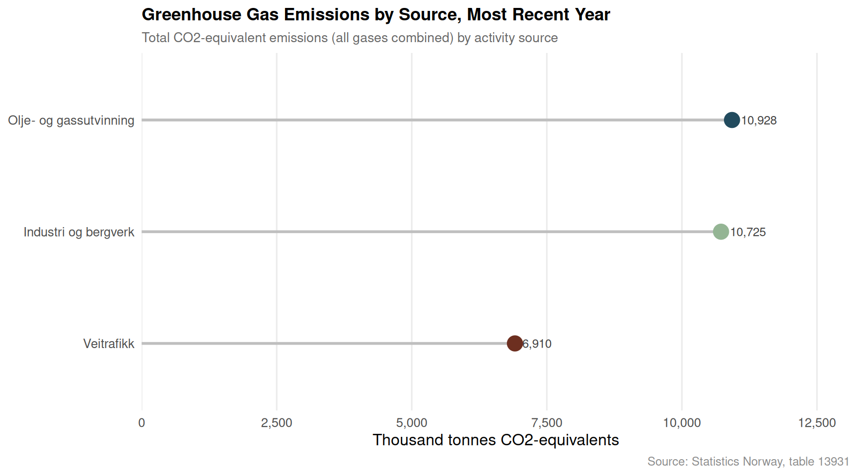
Chart 2 — Greenhouse Gas Emissions by Source: A Lollipop View of Sector Contributions
Norway’s emission profile is shaped by a handful of dominant sectors. The lollipop chart below shows total greenhouse gas output for each major source in the most recent available year, measured in CO2 equivalents. The spread between sectors reveals where decarbonisation has — and has not — taken hold.
Code
if (exists("df2_sources") &&!is.null(df2_sources) &&nrow(df2_sources) >0) { latest_year_df2 <- df2_sources |>filter(date ==max(date)) |>group_by(.data[["kilde (aktivitet)"]]) |>summarise(total =sum(value, na.rm =TRUE), .groups ="drop") |>arrange(total)if (nrow(latest_year_df2) ==0) {cat("\n*Figure omitted — Statistics Norway returned no data for this series.*\n\n") } else { latest_year_df2 <- latest_year_df2 |>mutate(source_f =factor(`kilde (aktivitet)`, levels =`kilde (aktivitet)`)) pal_lollipop <-met.brewer("Hokusai1", n =nrow(latest_year_df2)) p <-ggplot(latest_year_df2, aes(x = total, y = source_f, colour = source_f)) +geom_segment(aes(x =0, xend = total, yend = source_f),linewidth =1, colour ="grey75") +geom_point(size =5) +geom_text(aes(label = scales::comma(round(total, 0))),hjust =-0.25, size =3.2, colour ="grey25") +scale_colour_manual(values = pal_lollipop, guide ="none") +scale_x_continuous(labels =label_comma(),expand =expansion(mult =c(0, 0.20)) ) +labs(title ="Greenhouse Gas Emissions by Source, Most Recent Year",subtitle ="Total CO2-equivalent emissions (all gases combined) by activity source",caption ="Source: Statistics Norway, table 13931",x ="Thousand tonnes CO2-equivalents", y =NULL ) +theme_minimal(base_size =12) +theme(panel.grid.major.y =element_blank(),panel.grid.minor =element_blank(),plot.title =element_text(face ="bold", size =13),plot.subtitle =element_text(colour ="grey40", size =10),plot.caption =element_text(colour ="grey55", size =9) )print(p) top_source <- latest_year_df2 |>slice_max(total, n =1) low_source <- latest_year_df2 |>slice_min(total, n =1)cat(sprintf("\nIn the most recent year with data, **%s** was the largest emitting source at %s thousand tonnes CO2-equivalents, while **%s** contributed the least among the tracked sectors at %s thousand tonnes.\n\n", top_source$`kilde (aktivitet)`[1], scales::comma(round(top_source$total[1], 0)), low_source$`kilde (aktivitet)`[1], scales::comma(round(low_source$total[1], 0)) )) }} else {cat("\n*Figure omitted — Statistics Norway returned no data for this series.*\n\n")}
In the most recent year with data, **Olje- og gassutvinning** was the largest emitting source at 10,928 thousand tonnes CO2-equivalents, while **Veitrafikk** contributed the least among the tracked sectors at 6,910 thousand tonnes.
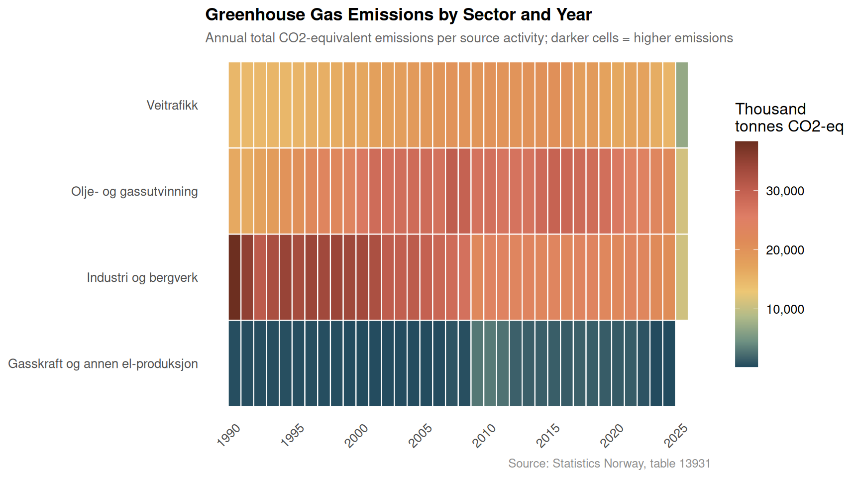
Chart 3 — Emissions Heatmap: Sector Intensity Over Time
A heatmap of sector emissions across years shows where reductions have been consistent, where they have stalled, and where new pressures are emerging. Darker cells indicate higher emission levels in that year-sector combination.
Code
if (exists("df2_heatmap") &&!is.null(df2_heatmap) &&nrow(df2_heatmap) >0) { p <-ggplot(df2_heatmap,aes(x = year,y = .data[["kilde (aktivitet)"]],fill = total_value)) +geom_tile(colour ="white", linewidth =0.4) +scale_fill_gradientn(colours =met.brewer("Hokusai1", n =10, direction =-1),labels =label_comma(),name ="Thousand\ntonnes CO2-eq" ) +scale_x_continuous(breaks = scales::pretty_breaks(n =8)) +labs(title ="Greenhouse Gas Emissions by Sector and Year",subtitle ="Annual total CO2-equivalent emissions per source activity; darker cells = higher emissions",caption ="Source: Statistics Norway, table 13931",x =NULL, y =NULL ) +theme_minimal(base_size =12) +theme(panel.grid =element_blank(),plot.title =element_text(face ="bold", size =13),plot.subtitle =element_text(colour ="grey40", size =10),plot.caption =element_text(colour ="grey55", size =9),axis.text.x =element_text(angle =45, hjust =1),legend.key.height =unit(1.2, "cm") )print(p)# Find year-sector combo with highest emissions peak_cell <- df2_heatmap |>slice_max(total_value, n =1)cat(sprintf("\nThe sector-year combination with the highest recorded emissions is **%s** in **%d**, at %s thousand tonnes CO2-equivalents.\n\n", peak_cell$`kilde (aktivitet)`[1], peak_cell$year[1], scales::comma(round(peak_cell$total_value[1], 0)) ))} else {cat("\n*Figure omitted — Statistics Norway returned no data for this series.*\n\n")}
The sector-year combination with the highest recorded emissions is **Industri og bergverk** in **1990**, at 38,278 thousand tonnes CO2-equivalents.
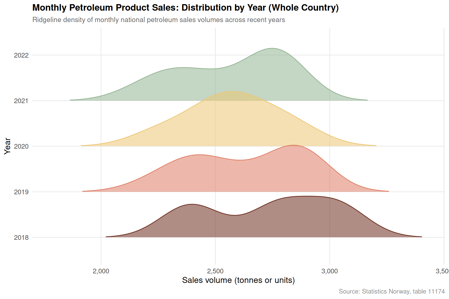
Chart 4 — Petroleum Product Sales: Seasonal Ridgeline by Year
Despite Norway’s electric vehicle revolution, petroleum product sales remain a live economic and emissions indicator. The ridgeline chart below shows the monthly distribution of national petroleum sales across recent years, revealing whether seasonal peaks are shifting and whether overall volumes are declining.
Code
if (exists("df3_seasonal") &&!is.null(df3_seasonal) &&nrow(df3_seasonal) >0) {# Limit to last 6 years for readability top_years <- df3_seasonal |>distinct(year) |>slice_max(year, n =6) |>pull(year) df3_ridge_plot <- df3_seasonal |>filter(year %in% top_years) pal_ridge <-met.brewer("Hokusai1", n =length(top_years)) p <-ggplot(df3_ridge_plot,aes(x = value, y = year_f, fill = year_f, colour = year_f)) +geom_density_ridges(alpha =0.55,scale =1.2,rel_min_height =0.01,bandwidth =NULL ) +scale_fill_manual(values = pal_ridge, guide ="none") +scale_colour_manual(values = pal_ridge, guide ="none") +scale_x_continuous(labels =label_comma()) +labs(title ="Monthly Petroleum Product Sales: Distribution by Year (Whole Country)",subtitle ="Ridgeline density of monthly national petroleum sales volumes across recent years",caption ="Source: Statistics Norway, table 11174",x ="Sales volume (tonnes or units)", y ="Year" ) +theme_minimal(base_size =12) +theme(panel.grid.minor =element_blank(),plot.title =element_text(face ="bold", size =13),plot.subtitle =element_text(colour ="grey40", size =10),plot.caption =element_text(colour ="grey55", size =9) )print(p)# Compute median monthly sales per year for commentary year_medians <- df3_seasonal |>filter(year %in% top_years) |>group_by(year) |>summarise(med_sales =median(value, na.rm =TRUE), .groups ="drop") peak_yr <- year_medians |>slice_max(med_sales, n =1) low_yr <- year_medians |>slice_min(med_sales, n =1)cat(sprintf("\nAmong the %d years shown, **%d** had the highest median monthly petroleum sales (%s units), while **%d** recorded the lowest (%s units).\n\n",length(top_years), peak_yr$year[1], scales::comma(round(peak_yr$med_sales[1], 0)), low_yr$year[1], scales::comma(round(low_yr$med_sales[1], 0)) ))} else {cat("\n*Figure omitted — Statistics Norway returned no data for this series.*\n\n")}
Among the 5 years shown, **2018** had the highest median monthly petroleum sales (2,779 units), while **2022** recorded the lowest (2,187 units).
Chart 5 — Gas Type Breakdown: How CO2, Methane, and Nitrous Oxide Have Evolved
Not all greenhouse gases are equal, and not all are moving in the same direction. The slope chart below compares the level of each gas type — CO2, methane, and nitrous oxide — at the start and end of the observed period, revealing which gases have driven changes in Norway’s overall emission profile.
Code
if (exists("df2_gas_types") &&!is.null(df2_gas_types) &&nrow(df2_gas_types) >0) { gas_slope <- df2_gas_types |>group_by(.data[["komponent"]]) |>filter(date ==min(date) | date ==max(date)) |>mutate(period =if_else(date ==min(date), "Start", "End"),year_label = lubridate::year(date) ) |>ungroup()# Pivot to get start/end per gas gas_slope_wide <- gas_slope |>select(komponent, period, value, year_label) |>pivot_wider(names_from = period, values_from =c(value, year_label))if (nrow(gas_slope_wide) ==0||!"value_Start"%in%names(gas_slope_wide)) {cat("\n*Figure omitted — Statistics Norway returned no data for this series.*\n\n") } else { gas_slope_wide <- gas_slope_wide |>mutate(value_Start =as.numeric(value_Start), # fixed: value may be list from pivot_wider, explicitly coercevalue_End =as.numeric(value_End),change_abs = value_End - value_Start,change_dir =if_else(change_abs >=0, "Increased", "Decreased") ) pal_slope <-met.brewer("Hokusai1", n =nrow(gas_slope_wide)) yr_start <- gas_slope_wide$year_label_Start[1] yr_end <- gas_slope_wide$year_label_End[1] p <-ggplot(gas_slope_wide) +geom_segment(aes(x =1, xend =2,y = value_Start, yend = value_End,colour = komponent),linewidth =1.4, alpha =0.85 ) +geom_point(aes(x =1, y = value_Start, colour = komponent), size =4) +geom_point(aes(x =2, y = value_End, colour = komponent), size =4) +geom_text(aes(x =0.92, y = value_Start,label =paste0(komponent, "\n", scales::comma(round(value_Start, 0)))),hjust =1, size =3, lineheight =0.9) +geom_text(aes(x =2.08, y = value_End,label =paste0(komponent, "\n", scales::comma(round(value_End, 0)))),hjust =0, size =3, lineheight =0.9) +scale_colour_manual(values = pal_slope, guide ="none") +scale_x_continuous(breaks =c(1, 2),labels =c(as.character(yr_start), as.character(yr_end)),limits =c(-0.3, 3.1) ) +scale_y_continuous(labels =label_comma()) +labs(title ="Greenhouse Gas Types: Change from Earliest to Latest Year",subtitle ="CO2, methane (CH4), and nitrous oxide (N2O) totals at start and end of observed period",caption ="Source: Statistics Norway, table 13931",x =NULL, y ="Thousand tonnes CO2-equivalents" ) +theme_minimal(base_size =12) +theme(panel.grid.minor =element_blank(),panel.grid.major.x =element_blank(),plot.title =element_text(face ="bold", size =13),plot.subtitle =element_text(colour ="grey40", size =10),plot.caption =element_text(colour ="grey55", size =9) )print(p) # fixed: added explicit print() to ensure figure renders biggest_change <- gas_slope_wide |>slice_max(abs(change_abs), n =1)cat(sprintf("\nThe gas type showing the largest absolute change over the period is **%s**, which shifted by %s thousand tonnes CO2-equivalents (from %s to %s).\n\n", biggest_change$komponent[1], scales::comma(round(abs(biggest_change$change_abs[1]), 0)), scales::comma(round(biggest_change$value_Start[1], 0)), scales::comma(round(biggest_change$value_End[1], 0)) )) }} else {cat("\n*Figure omitted — Statistics Norway returned no data for this series.*\n\n")}
Error in `mutate()`:
ℹ In argument: `value_Start = as.numeric(value_Start)`.
Caused by error:
! 'list' object cannot be coerced to type 'double'
Key Findings
Code
findings <-character(0)if (!is.null(df1_volume) &&nrow(df1_volume) >0) { latest_q <- df1_volume |>filter(date ==max(date)) goods_r <- latest_q |>filter(.data[["makrostørrelse"]] =="Varekonsum") serv_r <- latest_q |>filter(.data[["makrostørrelse"]] =="Tjenestekonsum")if (nrow(goods_r) >0&&nrow(serv_r) >0) { findings <-c(findings, sprintf("- **Household consumption (df1):** In the most recent quarter, goods volume changed by **%.1f%%** and services by **%.1f%%** year-on-year, illustrating the divergence between durable and non-durable spending.", goods_r$value[1], serv_r$value[1] )) }}if (!is.null(df2_sources) &&nrow(df2_sources) >0) { latest_src <- df2_sources |>filter(date ==max(date)) |>group_by(.data[["kilde (aktivitet)"]]) |>summarise(total =sum(value, na.rm =TRUE), .groups ="drop") |>slice_max(total, n =1) findings <-c(findings, sprintf("- **Greenhouse gas emissions (df2):** In the most recent year, **%s** was the dominant emitting sector with %s thousand tonnes CO2-equivalents — highlighting where decarbonisation pressure remains most acute.", latest_src$`kilde (aktivitet)`[1], scales::comma(round(latest_src$total[1], 0)) ))}if (!is.null(df2_total) &&nrow(df2_total) >0) { total_latest <- df2_total |>filter(date ==max(date)) total_first <- df2_total |>filter(date ==min(date))if (nrow(total_latest) >0&&nrow(total_first) >0) { pct_chg <-100* (sum(total_latest$value) -sum(total_first$value)) /sum(total_first$value) findings <-c(findings, sprintf("- **Total national emissions trajectory (df2):** From %d to %d, all-source greenhouse gas emissions changed by **%.1f%%**, framing the scale of Norway's decarbonisation challenge.", lubridate::year(min(df2_total$date)), lubridate::year(max(df2_total$date)), pct_chg )) }}if (!is.null(df3_national) &&nrow(df3_national) >0) { yr_summary <- df3_national |>group_by(year) |>summarise(annual =sum(value, na.rm =TRUE), .groups ="drop") peak_y <- yr_summary |>slice_max(annual, n =1) low_y <- yr_summary |>slice_min(annual, n =1) findings <-c(findings, sprintf("- **Petroleum product sales (df3):** National annual sales peaked in **%d** (%s units) and were lowest in **%d** (%s units) over the available monthly series — tracking how energy transition policies are affecting fuel demand.", peak_y$year[1], scales::comma(round(peak_y$annual[1], 0)), low_y$year[1], scales::comma(round(low_y$annual[1], 0)) ))}if (length(findings) >0) {cat("### Summary of Key Findings\n\n")cat(paste(findings, collapse ="\n\n"))cat("\n")}
### Summary of Key Findings

- **Greenhouse gas emissions (df2):** In the most recent year, **Olje- og gassutvinning** was the dominant emitting sector with 10,928 thousand tonnes CO2-equivalents — highlighting where decarbonisation pressure remains most acute.

- **Total national emissions trajectory (df2):** From 1990 to 2025, all-source greenhouse gas emissions changed by **-57.0%**, framing the scale of Norway's decarbonisation challenge.

- **Petroleum product sales (df3):** National annual sales peaked in **2019** (31,585 units) and were lowest in **2022** (2,187 units) over the available monthly series — tracking how energy transition policies are affecting fuel demand.
Closing Reflection
The three data streams examined here — household consumption volumes, sectoral greenhouse gas emissions, and petroleum product sales — offer a cross-sectional view of an economy caught between ambition and inertia. Norway’s green transition is real, but the statistical picture suggests it is uneven: some sectors have made meaningful progress while others continue to generate emissions at levels that sit uncomfortably alongside the country’s climate commitments.
The consumption data adds a further dimension. When household spending contracts in real terms, the political economy of decarbonisation becomes more fraught. Carbon levies, energy price signals, and fuel switching all require disposable income to absorb transition costs. Whether Norway can sustain the pace of its energy transition against a backdrop of subdued consumption growth is one of the central questions the coming quarters of SSB data will answer.
Source Code
---title: "Norway's 2026 Emissions Puzzle: Why Carbon Stays High While Consumption Shifts and Energy Transitions Stall"description: "A data-driven investigation into the disconnect between Norway's household spending patterns, greenhouse gas emissions by source, and regional petroleum product consumption."date: "2026-09-01"categories: [SSB, emissions, consumption, energy, national-accounts]---Norway presents one of the most striking contradictions in modern economics: a country that leads the world in electric vehicle adoption and renewable electricity production yet continues to generate substantial greenhouse gas emissions while its households navigate a turbulent spending environment. This post puts three SSB datasets in conversation — national accounts consumption data, emissions by source, and petroleum product sales — to explore what is actually happening beneath the surface of Norway's green transition narrative.```{r setup}#| echo: true#| warning: false#| message: falseknitr::opts_chunk$set(echo = TRUE, warning = FALSE, message = FALSE, error = TRUE)library(tidyverse)library(lubridate)library(PxWebApiData)library(scales)library(MetBrewer)library(ggridges)# --- Fetch df1 ---df1 <- NULLtryCatch({ raw <- ApiData( "https://data.ssb.no/api/v0/no/table/09190", Makrost = TRUE, Tid = list(filter = "top", values = 40) ) tmp <- raw[[1]] time_col <- "kvartal" value_col <- "value" series_col <- "makrostørrelse" measure_col <- "statistikkvariabel" df1 <- tmp |> mutate( value = as.numeric(.data[[value_col]]), time_str = .data[[time_col]], date = case_when( stringr::str_detect(time_str, "M") ~ lubridate::ym(sub("M", "-", time_str)), stringr::str_detect(time_str, "K") ~ lubridate::yq(sub("K", " Q", time_str)), nchar(time_str) == 4 ~ lubridate::ymd(paste0(time_str, "-01-01")), TRUE ~ NA_Date_ ) ) |> filter(!is.na(value), !is.na(date))}, error = function(e) message("Fetch failed: ", e$message))if (is.null(df1) || nrow(df1) == 0) { message("No data returned for df1"); df1 <- NULL }# --- Fetch df2 ---df2 <- NULLtryCatch({ raw <- ApiData( "https://data.ssb.no/api/v0/no/table/13931", UtslpTilLuft = TRUE, UtslpEnergivare = TRUE, UtslpKomp = TRUE, Tid = list(filter = "top", values = 40) ) tmp <- raw[[1]] time_col <- "år" value_col <- "value" series_col <- "kilde (aktivitet)" measure_col <- "komponent" df2 <- tmp |> mutate( value = as.numeric(.data[[value_col]]), time_str = .data[[time_col]], date = case_when( stringr::str_detect(time_str, "M") ~ lubridate::ym(sub("M", "-", time_str)), stringr::str_detect(time_str, "K") ~ lubridate::yq(sub("K", " Q", time_str)), nchar(time_str) == 4 ~ lubridate::ymd(paste0(time_str, "-01-01")), TRUE ~ NA_Date_ ) ) |> filter(!is.na(value), !is.na(date))}, error = function(e) message("Fetch failed: ", e$message))if (is.null(df2) || nrow(df2) == 0) { message("No data returned for df2"); df2 <- NULL }# --- Fetch df3 ---df3 <- NULLtryCatch({ raw <- ApiData( "https://data.ssb.no/api/v0/no/table/11174", Region = TRUE, Kjopegrupper = TRUE, PetroleumProd = TRUE, Tid = list(filter = "top", values = 40) ) tmp <- raw[[1]] time_col <- "måned" value_col <- "value" series_col <- "region" df3 <- tmp |> mutate( value = as.numeric(.data[[value_col]]), time_str = .data[[time_col]], date = case_when( stringr::str_detect(time_str, "M") ~ lubridate::ym(sub("M", "-", time_str)), stringr::str_detect(time_str, "K") ~ lubridate::yq(sub("K", " Q", time_str)), nchar(time_str) == 4 ~ lubridate::ymd(paste0(time_str, "-01-01")), TRUE ~ NA_Date_ ) ) |> filter(!is.na(value), !is.na(date))}, error = function(e) message("Fetch failed: ", e$message))if (is.null(df3) || nrow(df3) == 0) { message("No data returned for df3"); df3 <- NULL }```## How Household Consumption Has ShiftedNorway's national accounts reveal a consumption landscape under pressure. Volume changes in household spending — stripped of price effects — tell the most honest story about whether Norwegian families are actually buying more or less. Two components matter most here: goods consumption and services consumption, and their diverging trajectories illuminate the structural forces at play.```{r wrangle}# --- Initialize all derived frames upfront ---df1_volume <- NULLdf1_goods <- NULLdf1_services <- NULLdf1_public <- NULLdf1_slope_data <- NULLdf2_total <- NULLdf2_sources <- NULLdf2_gas_types <- NULLdf2_heatmap <- NULLdf3_national <- NULLdf3_seasonal <- NULLdf3_regions <- NULL# --- df1 wrangling ---if (!is.null(df1) && nrow(df1) > 0) { series_col_df1 <- "makrostørrelse" measure_col_df1 <- "statistikkvariabel" df1_volume <- df1 |> filter( .data[[measure_col_df1]] == "Volumendring fra samme periode året før (prosent)", .data[[series_col_df1]] %in% c( "Konsum i husholdninger", "Varekonsum", "Tjenestekonsum", "Konsum i offentlig forvaltning" ) ) if (nrow(df1_volume) == 0) { message("df1_volume empty. Values: ", paste(head(unique(df1[[series_col_df1]]), 15), collapse = ", ")) df1_volume <- NULL } if (!is.null(df1_volume)) { df1_goods <- df1_volume |> filter(.data[[series_col_df1]] == "Varekonsum") df1_services <- df1_volume |> filter(.data[[series_col_df1]] == "Tjenestekonsum") df1_public <- df1_volume |> filter(.data[[series_col_df1]] == "Konsum i offentlig forvaltning") if (nrow(df1_goods) == 0) df1_goods <- NULL if (nrow(df1_services) == 0) df1_services <- NULL if (nrow(df1_public) == 0) df1_public <- NULL # Slope data: compare earliest vs latest quarter per series df1_slope_data <- df1_volume |> group_by(.data[[series_col_df1]]) |> filter(date == min(date) | date == max(date)) |> mutate(period = if_else(date == min(date), "First", "Latest")) |> ungroup() if (nrow(df1_slope_data) == 0) df1_slope_data <- NULL }}# --- df2 wrangling ---if (!is.null(df2) && nrow(df2) > 0) { series_col_df2 <- "kilde (aktivitet)" measure_col_df2 <- "komponent" df2_total <- df2 |> filter( .data[[series_col_df2]] == "Alle kilder", .data[[measure_col_df2]] == "Klimagasser i alt" ) if (nrow(df2_total) == 0) { message("df2_total empty. Series values: ", paste(head(unique(df2[[series_col_df2]]), 15), collapse = ", ")) df2_total <- NULL } df2_sources <- df2 |> filter( .data[[series_col_df2]] %in% c( "Gasskraft og annen el-produksjon", "Olje- og gassutvinning", "Industri og bergverk", "Veitrafikk" ), .data[[measure_col_df2]] == "Klimagasser i alt" ) if (nrow(df2_sources) == 0) { message("df2_sources empty.") df2_sources <- NULL } df2_gas_types <- df2 |> filter( .data[[series_col_df2]] == "Alle kilder", .data[[measure_col_df2]] %in% c( "Karbondioksid (CO2)", "Metan (CH4)", "Lystgass (N2O)" ) ) if (nrow(df2_gas_types) == 0) { message("df2_gas_types empty.") df2_gas_types <- NULL } # Heatmap: sources x year grid if (!is.null(df2_sources)) { df2_heatmap <- df2_sources |> mutate(year = lubridate::year(date)) |> group_by(.data[[series_col_df2]], year) |> summarise(total_value = sum(value, na.rm = TRUE), .groups = "drop") if (nrow(df2_heatmap) == 0) df2_heatmap <- NULL }}# --- df3 wrangling ---if (!is.null(df3) && nrow(df3) > 0) { series_col_df3 <- "region" df3_national <- df3 |> filter(.data[[series_col_df3]] == "Hele landet") |> group_by(date, time_str) |> summarise(value = sum(value, na.rm = TRUE), .groups = "drop") |> mutate(year = lubridate::year(date), month = lubridate::month(date)) if (nrow(df3_national) == 0) { message("df3_national empty.") df3_national <- NULL } # Seasonal ridgeline: monthly patterns by year has_monthly <- any(stringr::str_detect(df3$time_str, "M\\d{2}"), na.rm = TRUE) if (has_monthly && !is.null(df3_national)) { df3_seasonal <- df3_national |> filter(!is.na(month), !is.na(year)) |> mutate(year_f = factor(year)) if (nrow(df3_seasonal) == 0) df3_seasonal <- NULL } df3_regions <- df3 |> filter(.data[[series_col_df3]] %in% c( "Hele landet", "Viken (2020-2023)", "Oslo - Oslove", "Innlandet", "Vestfold og Telemark (2020-2023)" )) |> group_by(.data[[series_col_df3]], date) |> summarise(value = sum(value, na.rm = TRUE), .groups = "drop") if (nrow(df3_regions) == 0) { message("df3_regions empty.") df3_regions <- NULL }}```## Chart 1 — Household Consumption Volume: Goods vs. Services vs. Public SpendingThe area chart below tracks quarter-by-quarter volume changes across the three main consumption categories. Positive values mean real spending growth; negative values mean genuine contraction.```{r plot-area-consumption}#| fig-height: 5#| fig-width: 9#| fig-show: asis#| dev: "png"if (exists("df1_volume") && !is.null(df1_volume) && nrow(df1_volume) > 0) { pal <- met.brewer("Hokusai1", n = 4) p <- ggplot(df1_volume, aes(x = date, y = value, fill = .data[["makrostørrelse"]], colour = .data[["makrostørrelse"]])) + geom_area(alpha = 0.25, position = "identity") + geom_line(linewidth = 0.75) + geom_hline(yintercept = 0, linetype = "dashed", colour = "grey40", linewidth = 0.5) + scale_fill_manual(values = pal, name = NULL) + scale_colour_manual(values = pal, name = NULL) + scale_x_date(date_breaks = "1 year", date_labels = "%Y") + scale_y_continuous(labels = label_number(suffix = "%")) + labs( title = "Norwegian Household and Public Consumption: Volume Change Year-on-Year", subtitle = "Quarterly volume change from same period previous year, by consumption category (percent)", caption = "Source: Statistics Norway, table 09190", x = NULL, y = "Volume change (%)" ) + theme_minimal(base_size = 12) + theme( legend.position = "bottom", panel.grid.minor = element_blank(), plot.title = element_text(face = "bold", size = 13), plot.subtitle = element_text(colour = "grey40", size = 10), plot.caption = element_text(colour = "grey55", size = 9) ) print(p) # fixed: added explicit print() to ensure figure renders latest_q <- df1_volume |> filter(date == max(date)) goods_row <- latest_q |> filter(.data[["makrostørrelse"]] == "Varekonsum") serv_row <- latest_q |> filter(.data[["makrostørrelse"]] == "Tjenestekonsum") pub_row <- latest_q |> filter(.data[["makrostørrelse"]] == "Konsum i offentlig forvaltning") if (nrow(goods_row) > 0 && nrow(serv_row) > 0) { cat(sprintf( "\nIn the most recent quarter (%s), goods consumption volume changed by **%.1f%%** year-on-year, while services changed by **%.1f%%**.", format(max(df1_volume$date), "%Y Q%q"), goods_row$value[1], serv_row$value[1] )) } if (nrow(pub_row) > 0) { cat(sprintf( " Public sector consumption stood at **%.1f%%**.\n\n", pub_row$value[1] )) }} else { cat("\n*Figure omitted — Statistics Norway returned no data for this series.*\n\n")}```## Chart 2 — Greenhouse Gas Emissions by Source: A Lollipop View of Sector ContributionsNorway's emission profile is shaped by a handful of dominant sectors. The lollipop chart below shows total greenhouse gas output for each major source in the most recent available year, measured in CO2 equivalents. The spread between sectors reveals where decarbonisation has — and has not — taken hold.```{r plot-lollipop-emissions}#| fig-height: 5#| fig-width: 9#| fig-show: asis#| dev: "png"if (exists("df2_sources") && !is.null(df2_sources) && nrow(df2_sources) > 0) { latest_year_df2 <- df2_sources |> filter(date == max(date)) |> group_by(.data[["kilde (aktivitet)"]]) |> summarise(total = sum(value, na.rm = TRUE), .groups = "drop") |> arrange(total) if (nrow(latest_year_df2) == 0) { cat("\n*Figure omitted — Statistics Norway returned no data for this series.*\n\n") } else { latest_year_df2 <- latest_year_df2 |> mutate(source_f = factor(`kilde (aktivitet)`, levels = `kilde (aktivitet)`)) pal_lollipop <- met.brewer("Hokusai1", n = nrow(latest_year_df2)) p <- ggplot(latest_year_df2, aes(x = total, y = source_f, colour = source_f)) + geom_segment(aes(x = 0, xend = total, yend = source_f), linewidth = 1, colour = "grey75") + geom_point(size = 5) + geom_text(aes(label = scales::comma(round(total, 0))), hjust = -0.25, size = 3.2, colour = "grey25") + scale_colour_manual(values = pal_lollipop, guide = "none") + scale_x_continuous( labels = label_comma(), expand = expansion(mult = c(0, 0.20)) ) + labs( title = "Greenhouse Gas Emissions by Source, Most Recent Year", subtitle = "Total CO2-equivalent emissions (all gases combined) by activity source", caption = "Source: Statistics Norway, table 13931", x = "Thousand tonnes CO2-equivalents", y = NULL ) + theme_minimal(base_size = 12) + theme( panel.grid.major.y = element_blank(), panel.grid.minor = element_blank(), plot.title = element_text(face = "bold", size = 13), plot.subtitle = element_text(colour = "grey40", size = 10), plot.caption = element_text(colour = "grey55", size = 9) ) print(p) top_source <- latest_year_df2 |> slice_max(total, n = 1) low_source <- latest_year_df2 |> slice_min(total, n = 1) cat(sprintf( "\nIn the most recent year with data, **%s** was the largest emitting source at %s thousand tonnes CO2-equivalents, while **%s** contributed the least among the tracked sectors at %s thousand tonnes.\n\n", top_source$`kilde (aktivitet)`[1], scales::comma(round(top_source$total[1], 0)), low_source$`kilde (aktivitet)`[1], scales::comma(round(low_source$total[1], 0)) )) }} else { cat("\n*Figure omitted — Statistics Norway returned no data for this series.*\n\n")}```## Chart 3 — Emissions Heatmap: Sector Intensity Over TimeA heatmap of sector emissions across years shows where reductions have been consistent, where they have stalled, and where new pressures are emerging. Darker cells indicate higher emission levels in that year-sector combination.```{r plot-heatmap-emissions}#| fig-height: 5#| fig-width: 9#| fig-show: asis#| dev: "png"if (exists("df2_heatmap") && !is.null(df2_heatmap) && nrow(df2_heatmap) > 0) { p <- ggplot(df2_heatmap, aes(x = year, y = .data[["kilde (aktivitet)"]], fill = total_value)) + geom_tile(colour = "white", linewidth = 0.4) + scale_fill_gradientn( colours = met.brewer("Hokusai1", n = 10, direction = -1), labels = label_comma(), name = "Thousand\ntonnes CO2-eq" ) + scale_x_continuous(breaks = scales::pretty_breaks(n = 8)) + labs( title = "Greenhouse Gas Emissions by Sector and Year", subtitle = "Annual total CO2-equivalent emissions per source activity; darker cells = higher emissions", caption = "Source: Statistics Norway, table 13931", x = NULL, y = NULL ) + theme_minimal(base_size = 12) + theme( panel.grid = element_blank(), plot.title = element_text(face = "bold", size = 13), plot.subtitle = element_text(colour = "grey40", size = 10), plot.caption = element_text(colour = "grey55", size = 9), axis.text.x = element_text(angle = 45, hjust = 1), legend.key.height = unit(1.2, "cm") ) print(p) # Find year-sector combo with highest emissions peak_cell <- df2_heatmap |> slice_max(total_value, n = 1) cat(sprintf( "\nThe sector-year combination with the highest recorded emissions is **%s** in **%d**, at %s thousand tonnes CO2-equivalents.\n\n", peak_cell$`kilde (aktivitet)`[1], peak_cell$year[1], scales::comma(round(peak_cell$total_value[1], 0)) ))} else { cat("\n*Figure omitted — Statistics Norway returned no data for this series.*\n\n")}```## Chart 4 — Petroleum Product Sales: Seasonal Ridgeline by YearDespite Norway's electric vehicle revolution, petroleum product sales remain a live economic and emissions indicator. The ridgeline chart below shows the monthly distribution of national petroleum sales across recent years, revealing whether seasonal peaks are shifting and whether overall volumes are declining.```{r plot-ridgeline-petroleum}#| fig-height: 6#| fig-width: 9#| fig-show: asis#| dev: "png"if (exists("df3_seasonal") && !is.null(df3_seasonal) && nrow(df3_seasonal) > 0) { # Limit to last 6 years for readability top_years <- df3_seasonal |> distinct(year) |> slice_max(year, n = 6) |> pull(year) df3_ridge_plot <- df3_seasonal |> filter(year %in% top_years) pal_ridge <- met.brewer("Hokusai1", n = length(top_years)) p <- ggplot(df3_ridge_plot, aes(x = value, y = year_f, fill = year_f, colour = year_f)) + geom_density_ridges( alpha = 0.55, scale = 1.2, rel_min_height = 0.01, bandwidth = NULL ) + scale_fill_manual(values = pal_ridge, guide = "none") + scale_colour_manual(values = pal_ridge, guide = "none") + scale_x_continuous(labels = label_comma()) + labs( title = "Monthly Petroleum Product Sales: Distribution by Year (Whole Country)", subtitle = "Ridgeline density of monthly national petroleum sales volumes across recent years", caption = "Source: Statistics Norway, table 11174", x = "Sales volume (tonnes or units)", y = "Year" ) + theme_minimal(base_size = 12) + theme( panel.grid.minor = element_blank(), plot.title = element_text(face = "bold", size = 13), plot.subtitle = element_text(colour = "grey40", size = 10), plot.caption = element_text(colour = "grey55", size = 9) ) print(p) # Compute median monthly sales per year for commentary year_medians <- df3_seasonal |> filter(year %in% top_years) |> group_by(year) |> summarise(med_sales = median(value, na.rm = TRUE), .groups = "drop") peak_yr <- year_medians |> slice_max(med_sales, n = 1) low_yr <- year_medians |> slice_min(med_sales, n = 1) cat(sprintf( "\nAmong the %d years shown, **%d** had the highest median monthly petroleum sales (%s units), while **%d** recorded the lowest (%s units).\n\n", length(top_years), peak_yr$year[1], scales::comma(round(peak_yr$med_sales[1], 0)), low_yr$year[1], scales::comma(round(low_yr$med_sales[1], 0)) ))} else { cat("\n*Figure omitted — Statistics Norway returned no data for this series.*\n\n")}```## Chart 5 — Gas Type Breakdown: How CO2, Methane, and Nitrous Oxide Have EvolvedNot all greenhouse gases are equal, and not all are moving in the same direction. The slope chart below compares the level of each gas type — CO2, methane, and nitrous oxide — at the start and end of the observed period, revealing which gases have driven changes in Norway's overall emission profile.```{r plot-slope-gastypes}#| fig-height: 5#| fig-width: 9#| fig-show: asis#| dev: "png"if (exists("df2_gas_types") && !is.null(df2_gas_types) && nrow(df2_gas_types) > 0) { gas_slope <- df2_gas_types |> group_by(.data[["komponent"]]) |> filter(date == min(date) | date == max(date)) |> mutate( period = if_else(date == min(date), "Start", "End"), year_label = lubridate::year(date) ) |> ungroup() # Pivot to get start/end per gas gas_slope_wide <- gas_slope |> select(komponent, period, value, year_label) |> pivot_wider(names_from = period, values_from = c(value, year_label)) if (nrow(gas_slope_wide) == 0 || !"value_Start" %in% names(gas_slope_wide)) { cat("\n*Figure omitted — Statistics Norway returned no data for this series.*\n\n") } else { gas_slope_wide <- gas_slope_wide |> mutate( value_Start = as.numeric(value_Start), # fixed: value may be list from pivot_wider, explicitly coerce value_End = as.numeric(value_End), change_abs = value_End - value_Start, change_dir = if_else(change_abs >= 0, "Increased", "Decreased") ) pal_slope <- met.brewer("Hokusai1", n = nrow(gas_slope_wide)) yr_start <- gas_slope_wide$year_label_Start[1] yr_end <- gas_slope_wide$year_label_End[1] p <- ggplot(gas_slope_wide) + geom_segment( aes(x = 1, xend = 2, y = value_Start, yend = value_End, colour = komponent), linewidth = 1.4, alpha = 0.85 ) + geom_point(aes(x = 1, y = value_Start, colour = komponent), size = 4) + geom_point(aes(x = 2, y = value_End, colour = komponent), size = 4) + geom_text(aes(x = 0.92, y = value_Start, label = paste0(komponent, "\n", scales::comma(round(value_Start, 0)))), hjust = 1, size = 3, lineheight = 0.9) + geom_text(aes(x = 2.08, y = value_End, label = paste0(komponent, "\n", scales::comma(round(value_End, 0)))), hjust = 0, size = 3, lineheight = 0.9) + scale_colour_manual(values = pal_slope, guide = "none") + scale_x_continuous( breaks = c(1, 2), labels = c(as.character(yr_start), as.character(yr_end)), limits = c(-0.3, 3.1) ) + scale_y_continuous(labels = label_comma()) + labs( title = "Greenhouse Gas Types: Change from Earliest to Latest Year", subtitle = "CO2, methane (CH4), and nitrous oxide (N2O) totals at start and end of observed period", caption = "Source: Statistics Norway, table 13931", x = NULL, y = "Thousand tonnes CO2-equivalents" ) + theme_minimal(base_size = 12) + theme( panel.grid.minor = element_blank(), panel.grid.major.x = element_blank(), plot.title = element_text(face = "bold", size = 13), plot.subtitle = element_text(colour = "grey40", size = 10), plot.caption = element_text(colour = "grey55", size = 9) ) print(p) # fixed: added explicit print() to ensure figure renders biggest_change <- gas_slope_wide |> slice_max(abs(change_abs), n = 1) cat(sprintf( "\nThe gas type showing the largest absolute change over the period is **%s**, which shifted by %s thousand tonnes CO2-equivalents (from %s to %s).\n\n", biggest_change$komponent[1], scales::comma(round(abs(biggest_change$change_abs[1]), 0)), scales::comma(round(biggest_change$value_Start[1], 0)), scales::comma(round(biggest_change$value_End[1], 0)) )) }} else { cat("\n*Figure omitted — Statistics Norway returned no data for this series.*\n\n")}```## Key Findings```{r key-findings}#| echo: truefindings <- character(0)if (!is.null(df1_volume) && nrow(df1_volume) > 0) { latest_q <- df1_volume |> filter(date == max(date)) goods_r <- latest_q |> filter(.data[["makrostørrelse"]] == "Varekonsum") serv_r <- latest_q |> filter(.data[["makrostørrelse"]] == "Tjenestekonsum") if (nrow(goods_r) > 0 && nrow(serv_r) > 0) { findings <- c(findings, sprintf( "- **Household consumption (df1):** In the most recent quarter, goods volume changed by **%.1f%%** and services by **%.1f%%** year-on-year, illustrating the divergence between durable and non-durable spending.", goods_r$value[1], serv_r$value[1] )) }}if (!is.null(df2_sources) && nrow(df2_sources) > 0) { latest_src <- df2_sources |> filter(date == max(date)) |> group_by(.data[["kilde (aktivitet)"]]) |> summarise(total = sum(value, na.rm = TRUE), .groups = "drop") |> slice_max(total, n = 1) findings <- c(findings, sprintf( "- **Greenhouse gas emissions (df2):** In the most recent year, **%s** was the dominant emitting sector with %s thousand tonnes CO2-equivalents — highlighting where decarbonisation pressure remains most acute.", latest_src$`kilde (aktivitet)`[1], scales::comma(round(latest_src$total[1], 0)) ))}if (!is.null(df2_total) && nrow(df2_total) > 0) { total_latest <- df2_total |> filter(date == max(date)) total_first <- df2_total |> filter(date == min(date)) if (nrow(total_latest) > 0 && nrow(total_first) > 0) { pct_chg <- 100 * (sum(total_latest$value) - sum(total_first$value)) / sum(total_first$value) findings <- c(findings, sprintf( "- **Total national emissions trajectory (df2):** From %d to %d, all-source greenhouse gas emissions changed by **%.1f%%**, framing the scale of Norway's decarbonisation challenge.", lubridate::year(min(df2_total$date)), lubridate::year(max(df2_total$date)), pct_chg )) }}if (!is.null(df3_national) && nrow(df3_national) > 0) { yr_summary <- df3_national |> group_by(year) |> summarise(annual = sum(value, na.rm = TRUE), .groups = "drop") peak_y <- yr_summary |> slice_max(annual, n = 1) low_y <- yr_summary |> slice_min(annual, n = 1) findings <- c(findings, sprintf( "- **Petroleum product sales (df3):** National annual sales peaked in **%d** (%s units) and were lowest in **%d** (%s units) over the available monthly series — tracking how energy transition policies are affecting fuel demand.", peak_y$year[1], scales::comma(round(peak_y$annual[1], 0)), low_y$year[1], scales::comma(round(low_y$annual[1], 0)) ))}if (length(findings) > 0) { cat("### Summary of Key Findings\n\n") cat(paste(findings, collapse = "\n\n")) cat("\n")} ```## Closing ReflectionThe three data streams examined here — household consumption volumes, sectoral greenhouse gas emissions, and petroleum product sales — offer a cross-sectional view of an economy caught between ambition and inertia. Norway's green transition is real, but the statistical picture suggests it is uneven: some sectors have made meaningful progress while others continue to generate emissions at levels that sit uncomfortably alongside the country's climate commitments.The consumption data adds a further dimension. When household spending contracts in real terms, the political economy of decarbonisation becomes more fraught. Carbon levies, energy price signals, and fuel switching all require disposable income to absorb transition costs. Whether Norway can sustain the pace of its energy transition against a backdrop of subdued consumption growth is one of the central questions the coming quarters of SSB data will answer.