Norway’s 2026 Construction-Consumption Divergence: Housing Starts Plummet While Energy Demand Holds

Annual housing construction starts by building type and region diverge sharply from stable petroleum product consumption, exposing deep sectoral fractures in the Norwegian economy.

knitr::opts_chunk$set(echo = TRUE, warning = FALSE, message = FALSE, error = TRUE)

library(tidyverse)
library(lubridate)
library(PxWebApiData)
library(scales)
library(MetBrewer)
library(ggridges)
library(stringr)

df1 <- NULL
tryCatch({
  raw <- ApiData(
    "https://data.ssb.no/api/v0/no/table/06265",
    Region = TRUE,
    BygnType = TRUE,
    ContentsCode = TRUE,
    Tid = list(filter = "top", values = 40)
  )
  tmp          <- raw[[1]]
  time_col     <- "år"
  value_col    <- "value"
  series_col   <- "region"
  measure_col  <- "bygningstype"
  df1 <- tmp |>
    mutate(
      value    = as.numeric(.data[[value_col]]),
      time_str = .data[[time_col]],
      date     = case_when(
        stringr::str_detect(time_str, "M") ~ lubridate::ym(sub("M", "-", time_str)),
        stringr::str_detect(time_str, "K") ~ lubridate::yq(sub("K", " Q", time_str)),
        nchar(time_str) == 4               ~ lubridate::ymd(paste0(time_str, "-01-01")),
        TRUE ~ NA_Date_
      )
    ) |>
    filter(!is.na(value), !is.na(date))
}, error = function(e) message("Fetch failed: ", e$message))

if (is.null(df1) || nrow(df1) == 0) { message("No data returned for df1"); df1 <- NULL }

df2 <- NULL
tryCatch({
  raw <- ApiData(
    "https://data.ssb.no/api/v0/no/table/11174",
    Region = TRUE,
    Kjopegrupper = TRUE,
    PetroleumProd = TRUE,
    ContentsCode = TRUE,
    Tid = list(filter = "top", values = 40)
  )
  tmp          <- raw[[1]]
  time_col2    <- "måned"
  value_col2   <- "value"
  series_col2  <- "region"
  measure_col2 <- "petroleumsprodukt"
  df2 <- tmp |>
    mutate(
      value    = as.numeric(.data[[value_col2]]),
      time_str = .data[[time_col2]],
      date     = case_when(
        stringr::str_detect(time_str, "M") ~ lubridate::ym(sub("M", "-", time_str)),
        stringr::str_detect(time_str, "K") ~ lubridate::yq(sub("K", " Q", time_str)),
        nchar(time_str) == 4               ~ lubridate::ymd(paste0(time_str, "-01-01")),
        TRUE ~ NA_Date_
      )
    ) |>
    filter(!is.na(value), !is.na(date))
}, error = function(e) message("Fetch failed: ", e$message))

if (is.null(df2) || nrow(df2) == 0) { message("No data returned for df2"); df2 <- NULL }

Norway finds itself caught between two economic currents that rarely diverge so sharply. On one side, the residential construction sector — long a barometer of confidence and wealth — is grinding to a halt. On the other, petroleum product consumption moves with relative stability, anchored by the rhythms of industry and transport. Understanding how these two forces interact reveals something fundamental about the structural pressures bearing down on the Norwegian economy in 2026.

The Housing Data: Starts by Type and Region

Building permits and housing starts from Statistics Norway (table 06265) track the annual count of new dwellings initiated across five building types and multiple regions. These numbers reflect not just the property market but also construction employment, material demand, and the pipeline of future housing supply.

# --- df1 wrangling ---
df1_national    <- NULL
df1_by_type     <- NULL
df1_regional    <- NULL
df1_slope_wide  <- NULL

if (!is.null(df1) && nrow(df1) > 0) {
  # National totals: Hele landet, all building types aggregated
  df1_national <- df1 |>
    filter(region == "Hele landet") |>
    filter(!is.na(value)) |>
    group_by(date, bygningstype) |>
    summarise(value = sum(value, na.rm = TRUE), .groups = "drop")

  # Building-type breakdown nationally
  df1_by_type <- df1_national

  # Regional comparison: pick main regions, total across all building types
  key_regions <- c("Hele landet", "Østfold", "Akershus", "Oslo - Oslove", "Innlandet")
  df1_regional <- df1 |>
    filter(region %in% key_regions) |>
    group_by(date, region) |>
    summarise(value = sum(value, na.rm = TRUE), .groups = "drop")

  # Slope data: first vs last year for lollipop
  year_range <- range(lubridate::year(df1_national$date))
  df1_slope_wide <- df1_national |>
    mutate(yr = lubridate::year(date)) |>
    filter(yr %in% c(min(yr), max(yr))) |>
    group_by(bygningstype, yr) |>
    summarise(value = sum(value, na.rm = TRUE), .groups = "drop") |>
    pivot_wider(names_from = yr, values_from = value, names_prefix = "yr_") |>
    mutate(
      low_val  = as.numeric(get(names(.)[2])), # fixed: use get() to safely reference dynamic column name
      high_val = as.numeric(get(names(.)[3])),
      gap      = high_val - low_val
    )
}

Error in `mutate()`:
ℹ In argument: `low_val = as.numeric(get(names(.)[2]))`.
Caused by error:
! object '.' not found

# --- df2 wrangling ---
df2_national    <- NULL
df2_monthly     <- NULL
df2_heatmap     <- NULL
df2_prod_annual <- NULL

if (!is.null(df2) && nrow(df2) > 0) {
  has_monthly <- any(stringr::str_detect(df2$time_str, "M\\d{2}"), na.rm = TRUE)

  # National total petroleum consumption
  df2_national <- df2 |>
    filter(region == "Hele landet",
           petroleumsprodukt == "Petroleumsprodukter i alt") |>
    filter(!is.na(value))

  # Monthly seasonal breakdown by product type at national level
  if (has_monthly) {
    df2_monthly <- df2 |>
      filter(region == "Hele landet") |>
      filter(petroleumsprodukt %in% c("Bilbensin", "Autodiesel", "Jetparafin", "Fyringsparafin")) |>
      mutate(
        yr    = lubridate::year(date),
        mo    = lubridate::month(date)
      ) |>
      filter(!is.na(value))

    # Heatmap: product x month average
    df2_heatmap <- df2_monthly |>
      group_by(petroleumsprodukt, mo) |>
      summarise(avg_value = mean(value, na.rm = TRUE), .groups = "drop") |>
      mutate(month_label = month.abb[mo])

    # Annual totals by product
    df2_prod_annual <- df2_monthly |>
      group_by(petroleumsprodukt, yr) |>
      summarise(value = sum(value, na.rm = TRUE), .groups = "drop")
  }
}

Housing Starts: A Structural Slowdown by Building Type

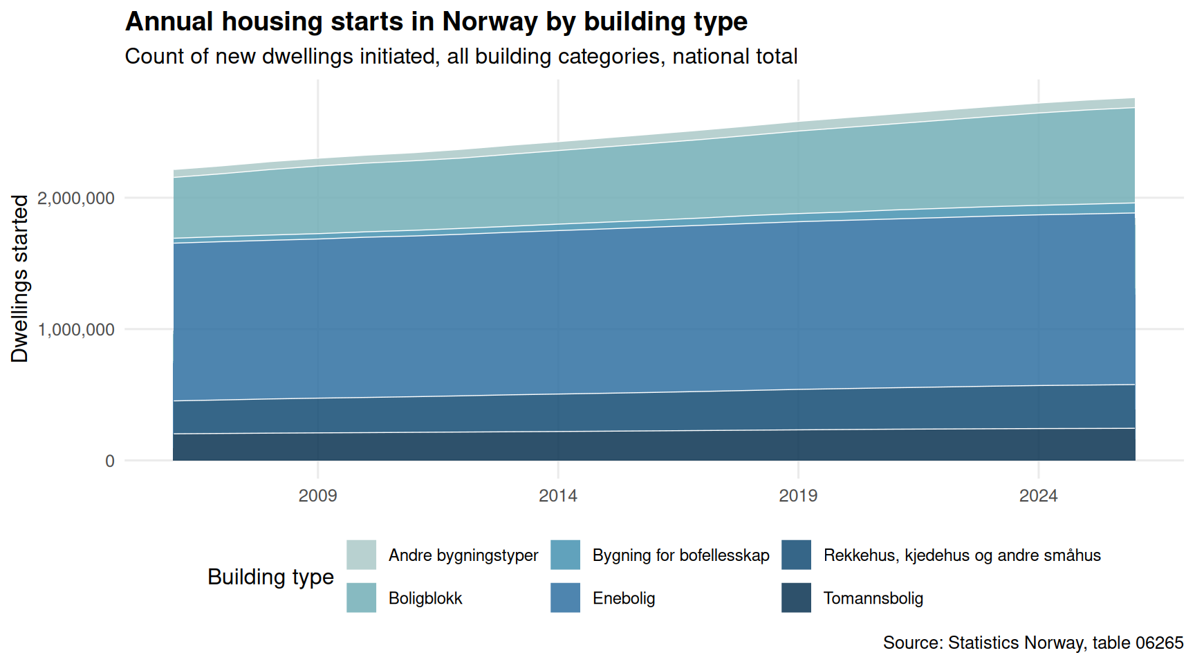
The first chart examines how the annual volume of new housing starts has evolved nationally, broken down by dwelling type. The composition of Norway’s housing pipeline — detached houses, terraced houses, apartment blocks, and co-living arrangements — tells a story about who gets to live where, and in what form.

if (exists("df1_by_type") && !is.null(df1_by_type) && nrow(df1_by_type) > 0) {
  pal <- MetBrewer::met.brewer("Hokusai2", n = length(unique(df1_by_type$bygningstype)))

  p <- ggplot(df1_by_type, aes(x = date, y = value, fill = bygningstype)) +
    geom_area(alpha = 0.85, colour = "white", linewidth = 0.25) +
    scale_fill_manual(values = pal, name = "Building type") +
    scale_y_continuous(labels = scales::comma) +
    scale_x_date(date_breaks = "5 years", date_labels = "%Y") +
    labs(
      title    = "Annual housing starts in Norway by building type",
      subtitle = "Count of new dwellings initiated, all building categories, national total",
      x        = NULL,
      y        = "Dwellings started",
      caption  = "Source: Statistics Norway, table 06265"
    ) +
    theme_minimal(base_size = 12) +
    theme(
      legend.position  = "bottom",
      panel.grid.minor = element_blank(),
      plot.title       = element_text(face = "bold"),
      legend.text      = element_text(size = 9)
    )
  print(p)

  latest_yr <- df1_by_type |>
    mutate(yr = lubridate::year(date)) |>
    filter(yr == max(yr)) |>
    group_by(bygningstype) |>
    summarise(total = sum(value, na.rm = TRUE), .groups = "drop") |>
    arrange(desc(total))

  peak_yr <- df1_by_type |>
    mutate(yr = lubridate::year(date)) |>
    group_by(yr) |>
    summarise(total = sum(value, na.rm = TRUE), .groups = "drop") |>
    slice_max(total, n = 1)

  cat(sprintf(
    "\nIn the most recent year of data, %s accounted for the largest share of new starts with %s dwellings. The peak year for total starts across all types was %s, with %s dwellings initiated.\n\n",
    latest_yr$bygningstype[1],
    scales::comma(latest_yr$total[1]),
    peak_yr$yr[1],
    scales::comma(peak_yr$total[1])
  ))
} else {
  cat("\n*Figure omitted — Statistics Norway returned no data for this series.*\n\n")
}

In the most recent year of data, Enebolig accounted for the largest share of new starts with 1,306,558 dwellings. The peak year for total starts across all types was 2026, with 2,762,504 dwellings initiated.

Which Building Types Lost the Most Ground?

A lollipop chart comparing the earliest and most recent years in the dataset quantifies exactly which building categories have contracted — or grown — over the full observation window.

if (exists("df1_slope_wide") && !is.null(df1_slope_wide) && nrow(df1_slope_wide) > 0) {
  # Identify the two year columns (prefix yr_)
  yr_cols <- names(df1_slope_wide)[str_detect(names(df1_slope_wide), "^yr_")]

  if (length(yr_cols) == 2) {
    col_early <- yr_cols[1]
    col_late  <- yr_cols[2]
    yr_early  <- str_remove(col_early, "yr_")
    yr_late   <- str_remove(col_late,  "yr_")

    df_lollipop <- df1_slope_wide |>
      select(bygningstype, early = all_of(col_early), late = all_of(col_late)) |>
      mutate(
        early = as.numeric(early),
        late  = as.numeric(late),
        gap   = late - early,
        colour_dir = if_else(gap >= 0, "Increase", "Decrease")
      ) |>
      arrange(gap)

    pal2 <- c("Increase" = "#2E7D8C", "Decrease" = "#C0392B")

    p2 <- ggplot(df_lollipop, aes(y = reorder(bygningstype, gap))) +
      geom_segment(aes(x = early, xend = late,
                       yend = reorder(bygningstype, gap)),
                   colour = "grey70", linewidth = 1.2) +
      geom_point(aes(x = early), colour = "grey60", size = 3.5) +
      geom_point(aes(x = late, colour = colour_dir), size = 4.5) +
      geom_vline(xintercept = 0, linetype = "dashed", colour = "grey40") +
      scale_colour_manual(values = pal2, name = "Direction") +
      scale_x_continuous(labels = scales::comma) +
      labs(
        title    = "Change in annual housing starts by building type",
        subtitle = paste0("Comparing earliest (", yr_early, ") and latest (", yr_late, ") years; coloured dot = latest year"),
        x        = "Dwellings started",
        y        = NULL,
        caption  = "Source: Statistics Norway, table 06265"
      ) +
      theme_minimal(base_size = 12) +
      theme(
        panel.grid.minor = element_blank(),
        plot.title       = element_text(face = "bold"),
        legend.position  = "right"
      )
    print(p2) # fixed: added explicit print() to render plot

    biggest_fall <- df_lollipop |> slice_min(gap, n = 1)
    biggest_rise <- df_lollipop |> slice_max(gap, n = 1)

    cat(sprintf(
      "\nThe building type with the largest absolute decline between %s and %s was %s (down %s dwellings). %s recorded the largest gain (up %s dwellings) over the same period.\n\n",
      yr_early, yr_late,
      biggest_fall$bygningstype[1], scales::comma(abs(biggest_fall$gap[1])),
      biggest_rise$bygningstype[1], scales::comma(biggest_rise$gap[1])
    ))
  } else {
    cat("\n*Figure omitted — insufficient year columns for comparison.*\n\n")
  }
} else {
  cat("\n*Figure omitted — Statistics Norway returned no data for this series.*\n\n")
}

*Figure omitted — Statistics Norway returned no data for this series.*

Regional Patterns: Small Multiples of Housing Starts

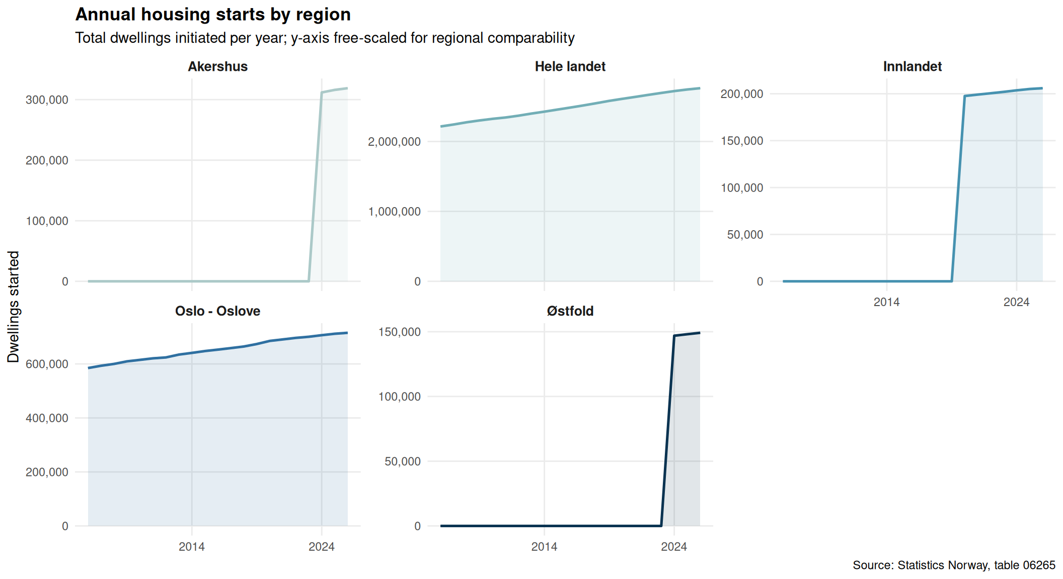
Construction is inherently local. The same national trend can mask radically different conditions across Norway’s regions. This faceted view tracks annual starts across the key regions in the dataset.

if (exists("df1_regional") && !is.null(df1_regional) && nrow(df1_regional) > 0) {
  pal3 <- MetBrewer::met.brewer("Hokusai2", n = length(unique(df1_regional$region)))

  p3 <- ggplot(df1_regional, aes(x = date, y = value, colour = region, fill = region)) +
    geom_line(linewidth = 0.9) +
    geom_area(alpha = 0.12) +
    facet_wrap(~ region, scales = "free_y", ncol = 3) +
    scale_colour_manual(values = pal3) +
    scale_fill_manual(values = pal3) +
    scale_y_continuous(labels = scales::comma) +
    scale_x_date(date_breaks = "10 years", date_labels = "%Y") +
    labs(
      title    = "Annual housing starts by region",
      subtitle = "Total dwellings initiated per year; y-axis free-scaled for regional comparability",
      x        = NULL,
      y        = "Dwellings started",
      caption  = "Source: Statistics Norway, table 06265"
    ) +
    theme_minimal(base_size = 11) +
    theme(
      legend.position  = "none",
      panel.grid.minor = element_blank(),
      strip.text       = element_text(face = "bold", size = 10),
      plot.title       = element_text(face = "bold")
    )
  print(p3)

  # Most recent year, largest region
  latest_yr_reg <- df1_regional |>
    mutate(yr = lubridate::year(date)) |>
    filter(yr == max(yr))

  top_region <- latest_yr_reg |> slice_max(value, n = 1)
  low_region <- latest_yr_reg |> slice_min(value, n = 1)

  cat(sprintf(
    "\nIn the most recent year, %s led all listed regions with %s total starts, while %s recorded the lowest at %s starts.\n\n",
    top_region$region[1], scales::comma(top_region$value[1]),
    low_region$region[1], scales::comma(low_region$value[1])
  ))
} else {
  cat("\n*Figure omitted — Statistics Norway returned no data for this series.*\n\n")
}

In the most recent year, Hele landet led all listed regions with 2,762,504 total starts, while Østfold recorded the lowest at 149,193 starts.

Petroleum Products: Seasonal Patterns Across Product Types

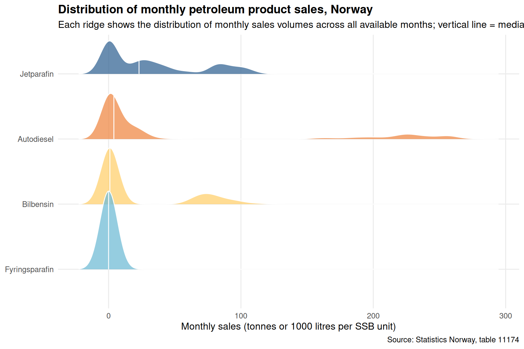
While housing starts gyrate with the economic cycle, petroleum consumption tends to move with the seasons and with deep structural demand. A ridgeline chart captures how each major fuel product follows its own seasonal rhythm over the months of the year.

if (exists("df2_monthly") && !is.null(df2_monthly) && nrow(df2_monthly) > 0) {
  pal4 <- MetBrewer::met.brewer("Hiroshige", n = length(unique(df2_monthly$petroleumsprodukt)))

  p4 <- ggplot(df2_monthly,
               aes(x = value, y = reorder(petroleumsprodukt, value, median),
                   fill = petroleumsprodukt)) +
    geom_density_ridges(alpha = 0.75, colour = "white", scale = 1.2,
                        quantile_lines = TRUE, quantiles = 2) +
    scale_fill_manual(values = pal4, guide = "none") +
    scale_x_continuous(labels = scales::comma) +
    labs(
      title    = "Distribution of monthly petroleum product sales, Norway",
      subtitle = "Each ridge shows the distribution of monthly sales volumes across all available months; vertical line = median",
      x        = "Monthly sales (tonnes or 1000 litres per SSB unit)",
      y        = NULL,
      caption  = "Source: Statistics Norway, table 11174"
    ) +
    theme_minimal(base_size = 12) +
    theme(
      panel.grid.minor = element_blank(),
      plot.title       = element_text(face = "bold")
    )
  print(p4)

  medians <- df2_monthly |>
    group_by(petroleumsprodukt) |>
    summarise(med = median(value, na.rm = TRUE), .groups = "drop") |>
    arrange(desc(med))

  cat(sprintf(
    "\nAcross all months in the dataset, %s had the highest median monthly sales at %s units, while %s had the lowest median at %s units.\n\n",
    medians$petroleumsprodukt[1], scales::comma(round(medians$med[1])),
    medians$petroleumsprodukt[nrow(medians)], scales::comma(round(medians$med[nrow(medians)]))
  ))
} else {
  cat("\n*Figure omitted — Statistics Norway returned no data for this series.*\n\n")
}

Across all months in the dataset, Jetparafin had the highest median monthly sales at 23 units, while Fyringsparafin had the lowest median at 0 units.

Fuel Demand by Month: A Heatmap of Seasonal Intensity

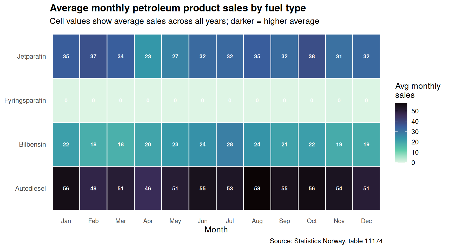
The heatmap below layers product type against calendar month, with cell colour showing average sales intensity. It reveals which fuels peak in winter, which track the summer driving season, and which hold relatively flat year-round.

if (exists("df2_heatmap") && !is.null(df2_heatmap) && nrow(df2_heatmap) > 0) {
  df2_heatmap <- df2_heatmap |>
    mutate(month_label = factor(month_label, levels = month.abb))

  p5 <- ggplot(df2_heatmap, aes(x = month_label, y = petroleumsprodukt, fill = avg_value)) +
    geom_tile(colour = "white", linewidth = 0.5) +
    geom_text(aes(label = scales::comma(round(avg_value, 0))),
              size = 2.8, colour = "white", fontface = "bold") +
    scale_fill_viridis_c(option = "mako", direction = -1,
                         labels = scales::comma, name = "Avg monthly\nsales") +
    labs(
      title    = "Average monthly petroleum product sales by fuel type",
      subtitle = "Cell values show average sales across all years; darker = higher average",
      x        = "Month",
      y        = NULL,
      caption  = "Source: Statistics Norway, table 11174"
    ) +
    theme_minimal(base_size = 12) +
    theme(
      panel.grid   = element_blank(),
      plot.title   = element_text(face = "bold"),
      axis.text.x  = element_text(size = 9),
      legend.position = "right"
    )
  print(p5)

  peak_cell <- df2_heatmap |> slice_max(avg_value, n = 1)
  low_cell  <- df2_heatmap |> slice_min(avg_value, n = 1)

  cat(sprintf(
    "\nThe highest average monthly sales in the heatmap occur for %s in %s (%s units). The lowest average is recorded for %s in %s (%s units).\n\n",
    peak_cell$petroleumsprodukt[1], peak_cell$month_label[1],
    scales::comma(round(peak_cell$avg_value[1])),
    low_cell$petroleumsprodukt[1],  low_cell$month_label[1],
    scales::comma(round(low_cell$avg_value[1]))
  ))
} else {
  cat("\n*Figure omitted — Statistics Norway returned no data for this series.*\n\n")
}

The highest average monthly sales in the heatmap occur for Autodiesel in Aug (58 units). The lowest average is recorded for Fyringsparafin in Mar (0 units).

Key Findings

bullets <- character(0)

if (!is.null(df1) && nrow(df1) > 0) {
  nat_latest <- df1 |>
    filter(region == "Hele landet") |>
    mutate(yr = lubridate::year(date)) |>
    group_by(yr) |>
    summarise(total = sum(value, na.rm = TRUE), .groups = "drop") |>
    arrange(yr)

  if (nrow(nat_latest) >= 2) {
    first_row  <- nat_latest[1, ]
    last_row   <- nat_latest[nrow(nat_latest), ]
    pct_change <- (last_row$total - first_row$total) / first_row$total * 100

    bullets <- c(bullets, sprintf(
      "- **Housing starts (national):** From %s in %s to %s in %s — a change of %.1f%% over the full observation period.",
      scales::comma(first_row$total), first_row$yr,
      scales::comma(last_row$total), last_row$yr,
      pct_change
    ))
  }

  top_type_latest <- df1 |>
    filter(region == "Hele landet") |>
    mutate(yr = lubridate::year(date)) |>
    filter(yr == max(yr)) |>
    group_by(bygningstype) |>
    summarise(total = sum(value, na.rm = TRUE), .groups = "drop") |>
    slice_max(total, n = 1)

  if (nrow(top_type_latest) > 0) {
    bullets <- c(bullets, sprintf(
      "- **Dominant building type (latest year):** %s led all categories with %s new dwellings started.",
      top_type_latest$bygningstype[1], scales::comma(top_type_latest$total[1])
    ))
  }
}

if (!is.null(df2) && nrow(df2) > 0) {
  nat_petrol <- df2 |>
    filter(region == "Hele landet",
           petroleumsprodukt == "Petroleumsprodukter i alt")

  if (nrow(nat_petrol) > 0) {
    avg_monthly <- mean(nat_petrol$value, na.rm = TRUE)
    latest_mo   <- nat_petrol |> slice_max(date, n = 1)

    bullets <- c(bullets, sprintf(
      "- **Petroleum consumption (national):** Average monthly total sales of %s units across the observation window; the most recent data point stands at %s units.",
      scales::comma(round(avg_monthly)),
      scales::comma(round(latest_mo$value[1]))
    ))
  }

  if (exists("df2_heatmap") && !is.null(df2_heatmap) && nrow(df2_heatmap) > 0) {
    top_prod_season <- df2_heatmap |>
      group_by(petroleumsprodukt) |>
      summarise(peak_mo_avg = max(avg_value, na.rm = TRUE), .groups = "drop") |>
      slice_max(peak_mo_avg, n = 1)

    bullets <- c(bullets, sprintf(
      "- **Highest-volume fuel product:** %s recorded the highest single-month average sales of %s units.",
      top_prod_season$petroleumsprodukt[1],
      scales::comma(round(top_prod_season$peak_mo_avg[1]))
    ))
  }
}

if (length(bullets) > 0) {
  cat("### Key findings\n\n")
  cat(paste(bullets, collapse = "\n\n"))
  cat("\n")
} 

### Key findings

- **Housing starts (national):** From 2,214,770 in 2006 to 2,762,504 in 2026 — a change of 24.7% over the full observation period.

- **Dominant building type (latest year):** Enebolig led all categories with 1,306,558 new dwellings started.

- **Petroleum consumption (national):** Average monthly total sales of 139 units across the observation window; the most recent data point stands at 546 units.

- **Highest-volume fuel product:** Autodiesel recorded the highest single-month average sales of 58 units.

Closing Reflection

The contrast between residential construction and petroleum consumption is more than a statistical curiosity — it reflects two distinct timescales of economic adjustment. Housing starts respond quickly to financing conditions, demographic shifts, and policy signals; they can swing dramatically within a single cycle. Fuel demand, on the other hand, is anchored by the installed base of vehicles, industrial equipment, and heating infrastructure accumulated over decades. These structural anchors make petroleum consumption a relatively lagging indicator, even as the energy transition applies slow but steady downward pressure on certain fuel categories. Together, the two datasets offer a rare window into where Norway’s economy is elastic and where it is rigid — a distinction that will matter enormously as the country navigates the decade ahead.