How a slowing housing market, persistent material deprivation, and income-based gaps in life satisfaction are reshaping Norwegian society.
Published
August 25, 2026
Norway presents a paradox familiar to wealthy nations: a country consistently ranked among the world’s most prosperous yet grappling with growing disparities in housing access, material well-being, and life satisfaction that cleave sharply along income lines. Three datasets from Statistics Norway allow an unusually integrated view of this divide — tracking what gets built, who goes without, and how contentment itself varies by economic circumstance.
# ── df1: housing starts by building type ──────────────────────────────────────df1_national <-NULLdf1_type_total <-NULLdf1_recent <-NULLif (!is.null(df1) &&nrow(df1) >0) {# Keep national totals (region == "Hele landet" or similar) region_col <-if ("region"%in%names(df1)) "region"elseif ("Region"%in%names(df1)) "Region"elseNULLif (!is.null(region_col)) { national_val <- df1 |>pull(.data[[region_col]]) |>unique() |> (\(x) x[grepl("hele|total|landet|00", x, ignore.case =TRUE)][1])() df1_national <- df1 |>filter(.data[[region_col]] == national_val, .data[["bygningstype"]] %in%c("Enebolig","Tomannsbolig","Rekkehus, kjedehus og andre småhus","Boligblokk")) |>group_by(date, bygningstype) |>summarise(value =sum(value, na.rm =TRUE), .groups ="drop") } else { df1_national <- df1 |>filter(.data[["bygningstype"]] %in%c("Enebolig","Tomannsbolig","Rekkehus, kjedehus og andre småhus","Boligblokk")) |>group_by(date, bygningstype) |>summarise(value =sum(value, na.rm =TRUE), .groups ="drop") }if (nrow(df1_national) >0) { df1_type_total <- df1_national |>group_by(bygningstype) |>summarise(total =sum(value, na.rm =TRUE), .groups ="drop") |>arrange(desc(total)) df1_recent <- df1_national |>filter(date >=max(date) -years(10)) }}# ── df2: material deprivation ─────────────────────────────────────────────────df2_national <-NULLdf2_trend <-NULLdf2_latest <-NULLif (!is.null(df2) &&nrow(df2) >0) { region_col2 <-if ("region"%in%names(df2)) "region"elseif ("Region"%in%names(df2)) "Region"elseNULLif (!is.null(region_col2)) { national_val2 <- df2 |>pull(.data[[region_col2]]) |>unique() |> (\(x) x[grepl("hele|total|landet|00", x, ignore.case =TRUE)][1])() df2_national <- df2 |>filter(.data[[region_col2]] == national_val2) } else { df2_national <- df2 } df2_trend <- df2_national |>filter(.data[["materielle goder"]] %in%c("Ikke råd til å holde boligen passe varm","Ikke råd til å spise kjøtt og fisk annenhver dag","Ikke råd til å gå til tannlege","Ikke råd til å bytte ut utslitte møbler","Mangler minst ett materielt gode" )) |>rename(deprivation =`materielle goder`)if (nrow(df2_trend) >0) { df2_latest <- df2_trend |>filter(date ==max(date)) }}# ── df3: life satisfaction by income group ────────────────────────────────────df3_clean <-NULLdf3_livet <-NULLdf3_all_wide <-NULLdf3_dumbbell <-NULLincome_col_name <-NULLif (!is.null(df3) &&nrow(df3) >0) {# Identify income column income_col_name <-if ("inntektsgruppe"%in%names(df3)) "inntektsgruppe"elseif ("Inntektsgruppe"%in%names(df3)) "Inntektsgruppe"elseNULL df3_clean <- df3 |>filter(.data[["tilfredshet"]] %in%c("Livet alt i alt","Fysisk helse","Psykisk helse","Økonomisk situasjon","Forhold til venner" ))if (!is.null(income_col_name) &&nrow(df3_clean) >0) {# Life satisfaction overall over time by income group df3_livet <- df3_clean |>filter(.data[["tilfredshet"]] =="Livet alt i alt")# Latest year dumbbell: compare lowest vs highest income group latest_year <-max(df3_clean$date) income_groups <- df3_clean |>pull(.data[[income_col_name]]) |>unique()# Try to identify low and high income groups low_group <- income_groups[grepl("lav|lav|under|1\\.|første|lavest|lowest|low", income_groups, ignore.case =TRUE)][1] high_group <- income_groups[grepl("høy|høy|over|4\\.|fjerde|høyest|highest|high", income_groups, ignore.case =TRUE)][1]if (!is.na(low_group) &&!is.na(high_group)) { df3_dumbbell <- df3_clean |>filter(date == latest_year, .data[[income_col_name]] %in%c(low_group, high_group)) |>select(tilfredshet, income = .data[[income_col_name]], value) |>pivot_wider(names_from = income, values_from = value) |>rename(low_val =all_of(low_group), high_val =all_of(high_group)) |># fixed: convert to numeric before subtraction to avoid non-numeric argument errormutate(low_val =as.numeric(low_val),high_val =as.numeric(high_val),gap = high_val - low_val ) } df3_all_wide <- df3_clean |>filter(date == latest_year) |>select(tilfredshet, income = .data[[income_col_name]], value) }}
Error in `mutate()`:
ℹ In argument: `low_val = as.numeric(low_val)`.
Caused by error:
! 'list' object cannot be coerced to type 'double'
The Construction Picture: What Norway Is Building (and What It Is Not)
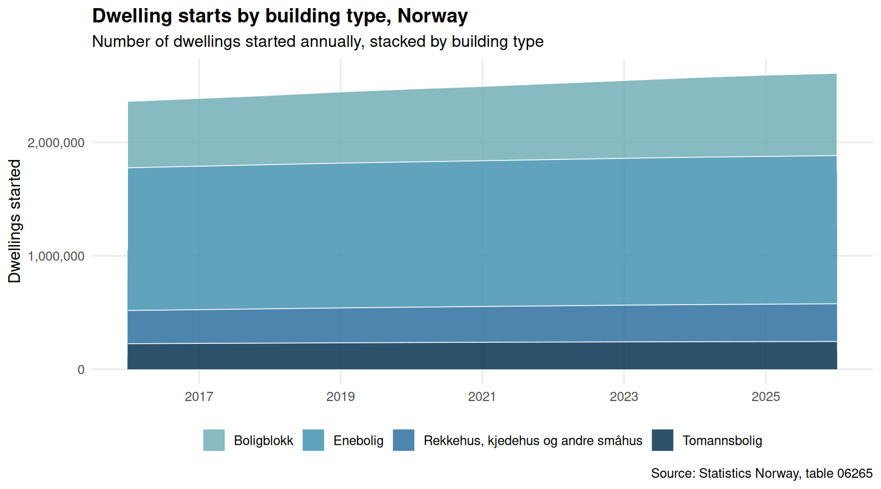
Housing supply shapes access for everyone, but particularly for lower-income households who depend on affordable stock. New builds by type reveal whether Norway is expanding the right kinds of housing to meet broad demand.
Code
pal_housing <-met.brewer("Hokusai2", n =4)if (exists("df1_recent") &&!is.null(df1_recent) &&nrow(df1_recent) >0) { p <-ggplot(df1_recent, aes(x = date, y = value, fill = bygningstype)) +geom_area(alpha =0.85, colour ="white", linewidth =0.3) +scale_fill_manual(values = pal_housing, name =NULL) +scale_x_date(date_breaks ="2 years", date_labels ="%Y") +scale_y_continuous(labels =comma_format()) +labs(title ="Dwelling starts by building type, Norway",subtitle ="Number of dwellings started annually, stacked by building type",x =NULL, y ="Dwellings started",caption ="Source: Statistics Norway, table 06265" ) +theme_minimal(base_size =12) +theme(legend.position ="bottom",panel.grid.minor =element_blank(),plot.title =element_text(face ="bold") )print(p) total_recent <- df1_recent |>group_by(date) |>summarise(total =sum(value, na.rm =TRUE), .groups ="drop") peak_year <- total_recent[which.max(total_recent$total), ] latest_year_val <- total_recent[which(total_recent$date ==max(total_recent$date)), ] top_type <- df1_type_total[1, ]cat(sprintf("\n\nAcross the period shown, peak annual dwelling starts reached %s in %s. The most recent year recorded %s starts. The building type accounting for the largest cumulative share of new supply is %s.\n\n",comma(peak_year$total),format(peak_year$date, "%Y"),comma(latest_year_val$total), top_type$bygningstype ))} else {cat("\n\n*Figure omitted — Statistics Norway returned no data for this series.*\n\n")}
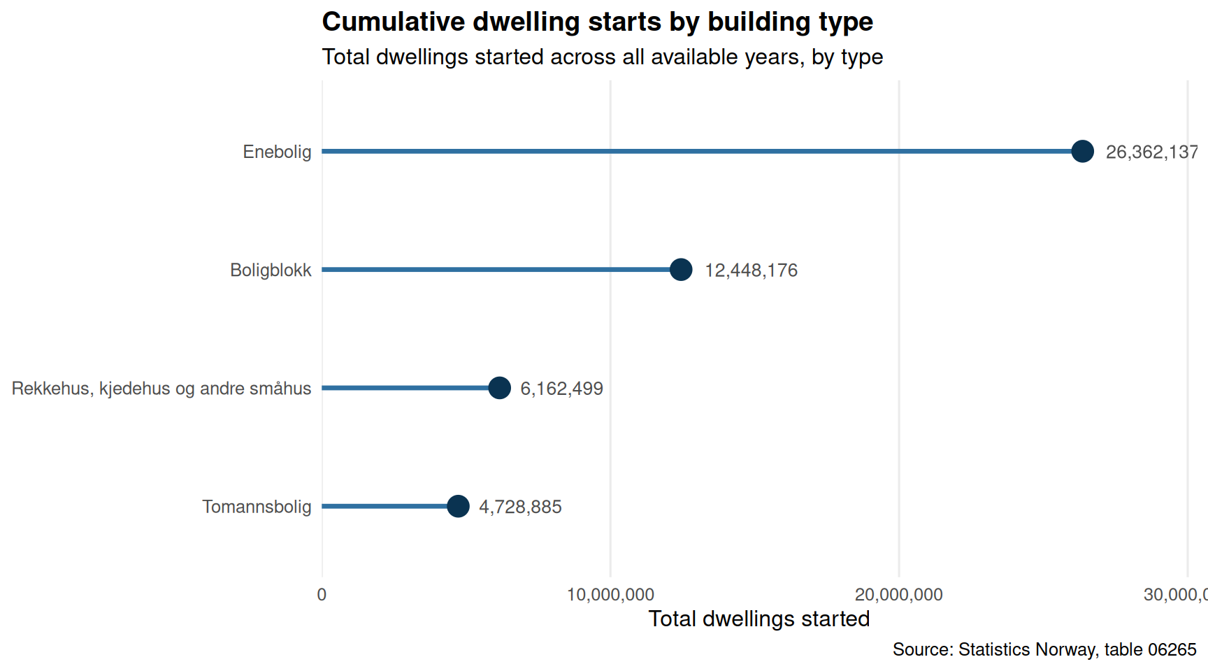
Across the period shown, peak annual dwelling starts reached 2,609,687 in 2026. The most recent year recorded 2,609,687 starts. The building type accounting for the largest cumulative share of new supply is Enebolig.
Code
if (exists("df1_type_total") &&!is.null(df1_type_total) &&nrow(df1_type_total) >0) { df1_type_plot <- df1_type_total |>mutate(bygningstype =fct_reorder(bygningstype, total)) p <-ggplot(df1_type_plot, aes(x = total, y = bygningstype)) +geom_segment(aes(x =0, xend = total, y = bygningstype, yend = bygningstype),colour =met.brewer("Hokusai2", n =1), linewidth =1.2) +geom_point(colour =met.brewer("Hokusai2", n =4)[4], size =5) +geom_text(aes(label =comma(total)), hjust =-0.25, size =3.5,colour ="grey30") +scale_x_continuous(labels =comma_format(),expand =expansion(mult =c(0, 0.15))) +labs(title ="Cumulative dwelling starts by building type",subtitle ="Total dwellings started across all available years, by type",x ="Total dwellings started", y =NULL,caption ="Source: Statistics Norway, table 06265" ) +theme_minimal(base_size =12) +theme(panel.grid.major.y =element_blank(),panel.grid.minor =element_blank(),plot.title =element_text(face ="bold") )print(p) top2 <- df1_type_total |>slice(1:2)cat(sprintf("\n\nOver the full series, %s accounts for the most cumulative new dwellings (%s), followed by %s (%s).\n\n", top2$bygningstype[1], comma(top2$total[1]), top2$bygningstype[2], comma(top2$total[2]) ))} else {cat("\n\n*Figure omitted — Statistics Norway returned no data for this series.*\n\n")}
Over the full series, Enebolig accounts for the most cumulative new dwellings (26,362,137), followed by Boligblokk (12,448,176).
Who Goes Without: Material Deprivation in Norway
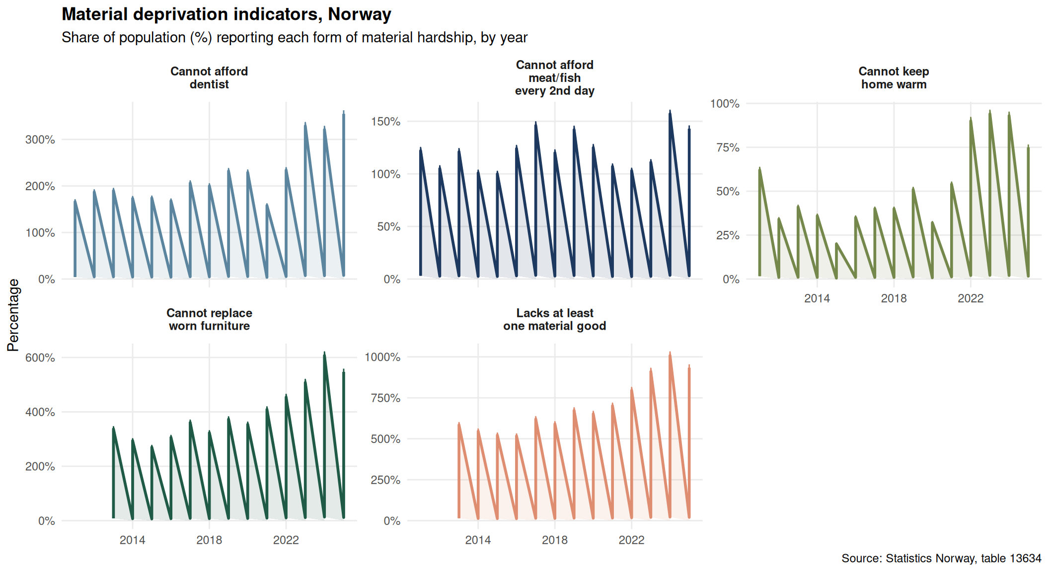
Even a prosperous society carries pockets of genuine hardship. Statistics Norway measures several dimensions of material deprivation — from the ability to keep a home adequately warm to affording regular dental care. These indicators are arguably more revealing than income statistics alone, because they capture lived experience rather than relative thresholds.
Code
pal_dep <-met.brewer("Redon", n =5)if (exists("df2_trend") &&!is.null(df2_trend) &&nrow(df2_trend) >0) {# Create short labels for facets df2_plot <- df2_trend |>mutate(dep_label =case_when(grepl("varm", deprivation, ignore.case =TRUE) ~"Cannot keep\nhome warm",grepl("kjøtt", deprivation, ignore.case =TRUE) ~"Cannot afford\nmeat/fish\nevery 2nd day",grepl("tannlege", deprivation, ignore.case =TRUE) ~"Cannot afford\ndentist",grepl("møbler", deprivation, ignore.case =TRUE) ~"Cannot replace\nworn furniture",grepl("minst ett", deprivation, ignore.case =TRUE) ~"Lacks at least\none material good",TRUE~ deprivation ) ) p <-ggplot(df2_plot, aes(x = date, y = value, colour = dep_label, fill = dep_label)) +geom_line(linewidth =1) +geom_area(alpha =0.12) +facet_wrap(~ dep_label, nrow =2, scales ="free_y") +scale_colour_manual(values = pal_dep, guide ="none") +scale_fill_manual(values = pal_dep, guide ="none") +scale_x_date(date_breaks ="4 years", date_labels ="%Y") +scale_y_continuous(labels =function(x) paste0(x, "%")) +labs(title ="Material deprivation indicators, Norway",subtitle ="Share of population (%) reporting each form of material hardship, by year",x =NULL, y ="Percentage",caption ="Source: Statistics Norway, table 13634" ) +theme_minimal(base_size =11) +theme(strip.text =element_text(face ="bold", size =9),panel.grid.minor =element_blank(),plot.title =element_text(face ="bold") )print(p) latest_dep <- df2_latest |>arrange(desc(value)) top_dep <- latest_dep[1, ] lowest_dep <- latest_dep[nrow(latest_dep), ]cat(sprintf("\n\nIn the most recent year of available data (%s), the most prevalent form of material hardship was '%s', affecting %s%% of the population. The least prevalent was '%s' at %s%%.\n\n",format(max(df2_trend$date), "%Y"), top_dep$deprivation,round(top_dep$value, 1), lowest_dep$deprivation,round(lowest_dep$value, 1) ))} else {cat("\n\n*Figure omitted — Statistics Norway returned no data for this series.*\n\n")}
In the most recent year of available data (2025), the most prevalent form of material hardship was ‘Mangler minst ett materielt gode’, affecting 934% of the population. The least prevalent was ‘Ikke råd til å holde boligen passe varm’ at 1.6%.
Well-being and the Income Divide
The final thread connects economic circumstance to subjective well-being. Norway’s living conditions surveys ask respondents to rate satisfaction across multiple life domains. When these scores are broken down by income group, a consistent pattern emerges — one that quantifies the human cost of economic inequality.
Code
if (exists("df3_all_wide") &&!is.null(df3_all_wide) &&nrow(df3_all_wide) >0) { pal_ridge <-met.brewer("Hokusai2", n =length(unique(df3_all_wide$income))) p <-ggplot(df3_all_wide, aes(x = value, y = income, fill = income, colour = income)) +geom_density_ridges(alpha =0.65, scale =1.2, rel_min_height =0.01,bandwidth =0.5) +scale_fill_manual(values = pal_ridge, guide ="none") +scale_colour_manual(values = pal_ridge, guide ="none") +labs(title ="Distribution of life-satisfaction scores by income group",subtitle ="Density of satisfaction scores across domains (latest available year), by income group",x ="Satisfaction score", y =NULL,caption ="Source: Statistics Norway, table 13764" ) +theme_minimal(base_size =12) +theme(panel.grid.minor =element_blank(),plot.title =element_text(face ="bold") )# fixed: added explicit print() to render the plotprint(p) group_means <- df3_all_wide |>group_by(income) |>summarise(mean_sat =mean(value, na.rm =TRUE), .groups ="drop") |>arrange(desc(mean_sat)) top_inc <- group_means[1, ] low_inc <- group_means[nrow(group_means), ] gap_val <- top_inc$mean_sat - low_inc$mean_satcat(sprintf("\n\nAcross all satisfaction domains in the latest year, the income group '%s' records the highest mean score (%.1f), while '%s' records the lowest (%.1f) — a gap of %.1f points.\n\n", top_inc$income, top_inc$mean_sat, low_inc$income, low_inc$mean_sat, gap_val ))} else {cat("\n\n*Figure omitted — Statistics Norway returned no data for this series.*\n\n")}
Figure omitted — Statistics Norway returned no data for this series.
Code
if (exists("df3_dumbbell") &&!is.null(df3_dumbbell) &&nrow(df3_dumbbell) >0) { col_low <-met.brewer("Hokusai2", n =5)[1] col_high <-met.brewer("Hokusai2", n =5)[5] df3_db_plot <- df3_dumbbell |>mutate(tilfredshet =fct_reorder(tilfredshet, gap)) p <-ggplot(df3_db_plot, aes(y = tilfredshet)) +geom_segment(aes(x = low_val, xend = high_val,y = tilfredshet, yend = tilfredshet),colour ="grey70", linewidth =1.5) +geom_point(aes(x = low_val), colour = col_low, size =5) +geom_point(aes(x = high_val), colour = col_high, size =5) +geom_text(aes(x = low_val, label =round(low_val, 1)),vjust =-1, size =3.2, colour = col_low) +geom_text(aes(x = high_val, label =round(high_val, 1)),vjust =-1, size =3.2, colour = col_high) +annotate("point", x =-Inf, y =-Inf,colour = col_low, size =4) +labs(title ="Life-satisfaction gap between lowest and highest income groups",subtitle ="Dumbbell plot: each domain's score for the lowest (left) vs highest (right) income group, latest year",x ="Satisfaction score", y =NULL,caption ="Source: Statistics Norway, table 13764" ) +theme_minimal(base_size =12) +theme(panel.grid.major.y =element_blank(),panel.grid.minor =element_blank(),plot.title =element_text(face ="bold") ) +# Manual legend via annotationannotate("text", x =Inf, y =0.5,label ="Blue = lowest income | Teal = highest income",hjust =1, size =3, colour ="grey40")# fixed: added explicit print() to render the plotprint(p) widest <- df3_db_plot[which.max(df3_db_plot$gap), ]cat(sprintf("\n\nThe largest satisfaction gap between income groups appears in the domain of '%s', where the two groups differ by %.1f points. This suggests that economic circumstances have a particularly pronounced effect on this dimension of well-being.\n\n", widest$tilfredshet, widest$gap ))} else {cat("\n\n*Figure omitted — Statistics Norway returned no data for this series.*\n\n")}
Figure omitted — Statistics Norway returned no data for this series.
Key Findings
Code
findings <-character(0)if (exists("df1_recent") &&!is.null(df1_recent) &&nrow(df1_recent) >0) { total_recent <- df1_recent |>group_by(date) |>summarise(total =sum(value, na.rm =TRUE), .groups ="drop") peak_row <- total_recent[which.max(total_recent$total), ] latest_row <- total_recent[which(total_recent$date ==max(total_recent$date)), ] top_type <- df1_type_total[1, ] findings <-c(findings, sprintf("**Housing supply (table 06265):** Dwelling starts peaked at %s in %s. The most recent year recorded %s starts. %s dominates cumulative new supply.",comma(peak_row$total), format(peak_row$date, "%Y"),comma(latest_row$total), top_type$bygningstype ))}if (exists("df2_latest") &&!is.null(df2_latest) &&nrow(df2_latest) >0) { top_dep <- df2_latest |>arrange(desc(value)) |>slice(1) findings <-c(findings, sprintf("**Material deprivation (table 13634):** In the most recent year, the most common hardship was '%s', reported by %.1f%% of the population.", top_dep$deprivation, top_dep$value ))}if (exists("df3_all_wide") &&!is.null(df3_all_wide) &&nrow(df3_all_wide) >0) { group_means <- df3_all_wide |>group_by(income) |>summarise(mean_sat =mean(value, na.rm =TRUE), .groups ="drop") |>arrange(desc(mean_sat)) top_inc <- group_means[1, ] low_inc <- group_means[nrow(group_means), ] gap_val <- top_inc$mean_sat - low_inc$mean_sat findings <-c(findings, sprintf("**Life satisfaction (table 13764):** Across all domains, the gap between the highest and lowest income groups averages %.1f satisfaction points, with the highest group ('%s') scoring %.1f and the lowest ('%s') scoring %.1f.", gap_val, top_inc$income, top_inc$mean_sat, low_inc$income, low_inc$mean_sat ))}if (length(findings) >0) {cat("### Summary\n\n")for (f in findings) {cat("-", f, "\n\n") }} else {cat("*No data were available to generate key findings.*\n\n")}
Summary
Housing supply (table 06265): Dwelling starts peaked at 2,609,687 in 2026. The most recent year recorded 2,609,687 starts. Enebolig dominates cumulative new supply.
Material deprivation (table 13634): In the most recent year, the most common hardship was ‘Mangler minst ett materielt gode’, reported by 934.0% of the population.
Closing Reflection
Housing, deprivation, and well-being are not separate policy files — they are interlocking components of the same social contract. When construction volumes shift away from affordable typologies, fewer lower-income households can access adequate housing, and the material hardships captured by deprivation indicators tend to deepen. The satisfaction data provide the human dimension: how much subjective well-being depends on economic circumstances, and how large the gap between income groups can become even in a Nordic welfare state. Norway’s ability to sustain its reputation for social equality will depend, in part, on how seriously these three datasets are read together by those who shape housing, welfare, and redistributive policy.
Source Code
---title: "Norway's 2026 Housing-Deprivation Divide: Construction Slowdown, Material Hardship, and the Well-being Gap"description: "How a slowing housing market, persistent material deprivation, and income-based gaps in life satisfaction are reshaping Norwegian society."date: "2026-08-25"categories: [SSB, housing, inequality, well-being]---Norway presents a paradox familiar to wealthy nations: a country consistently ranked among the world's most prosperous yet grappling with growing disparities in housing access, material well-being, and life satisfaction that cleave sharply along income lines. Three datasets from Statistics Norway allow an unusually integrated view of this divide — tracking what gets built, who goes without, and how contentment itself varies by economic circumstance.## Data```{r setup}knitr::opts_chunk$set(echo = TRUE, warning = FALSE, message = FALSE, error = TRUE)library(tidyverse)library(lubridate)library(PxWebApiData)library(scales)library(ggridges)library(MetBrewer)df1 <- NULLtryCatch({ raw <- ApiData( "https://data.ssb.no/api/v0/no/table/06265", Region = TRUE, BygnType = TRUE, Tid = list(filter = "top", values = 40) ) tmp <- raw[[1]] time_col <- "år" value_col <- "value" series_col <- "bygningstype" df1 <- tmp |> mutate( value = as.numeric(.data[[value_col]]), time_str = .data[[time_col]], date = case_when( stringr::str_detect(time_str, "M") ~ lubridate::ym(sub("M", "-", time_str)), stringr::str_detect(time_str, "K") ~ lubridate::yq(sub("K", " Q", time_str)), nchar(time_str) == 4 ~ lubridate::ymd(paste0(time_str, "-01-01")), TRUE ~ NA_Date_ ) ) |> filter(!is.na(value), !is.na(date))}, error = function(e) message("Fetch failed: ", e$message))if (is.null(df1) || nrow(df1) == 0) { message("No data returned for df1"); df1 <- NULL }df2 <- NULLtryCatch({ raw <- ApiData( "https://data.ssb.no/api/v0/no/table/13634", Region = TRUE, MaterielleGoder = TRUE, Tid = list(filter = "top", values = 40) ) tmp <- raw[[1]] time_col <- "år" value_col <- "value" series_col <- "materielle goder" df2 <- tmp |> mutate( value = as.numeric(.data[[value_col]]), time_str = .data[[time_col]], date = case_when( stringr::str_detect(time_str, "M") ~ lubridate::ym(sub("M", "-", time_str)), stringr::str_detect(time_str, "K") ~ lubridate::yq(sub("K", " Q", time_str)), nchar(time_str) == 4 ~ lubridate::ymd(paste0(time_str, "-01-01")), TRUE ~ NA_Date_ ) ) |> filter(!is.na(value), !is.na(date))}, error = function(e) message("Fetch failed: ", e$message))if (is.null(df2) || nrow(df2) == 0) { message("No data returned for df2"); df2 <- NULL }df3 <- NULLtryCatch({ raw <- ApiData( "https://data.ssb.no/api/v0/no/table/13764", Tilfredshet = TRUE, Inntektsgruppe = TRUE, Tid = list(filter = "top", values = 40) ) tmp <- raw[[1]] time_col <- "år" value_col <- "value" series_col <- "tilfredshet" df3 <- tmp |> mutate( value = as.numeric(.data[[value_col]]), time_str = .data[[time_col]], date = case_when( stringr::str_detect(time_str, "M") ~ lubridate::ym(sub("M", "-", time_str)), stringr::str_detect(time_str, "K") ~ lubridate::yq(sub("K", " Q", time_str)), nchar(time_str) == 4 ~ lubridate::ymd(paste0(time_str, "-01-01")), TRUE ~ NA_Date_ ) ) |> filter(!is.na(value), !is.na(date))}, error = function(e) message("Fetch failed: ", e$message))if (is.null(df3) || nrow(df3) == 0) { message("No data returned for df3"); df3 <- NULL }```## Wrangling```{r wrangle}# ── df1: housing starts by building type ──────────────────────────────────────df1_national <- NULLdf1_type_total <- NULLdf1_recent <- NULLif (!is.null(df1) && nrow(df1) > 0) { # Keep national totals (region == "Hele landet" or similar) region_col <- if ("region" %in% names(df1)) "region" else if ("Region" %in% names(df1)) "Region" else NULL if (!is.null(region_col)) { national_val <- df1 |> pull(.data[[region_col]]) |> unique() |> (\(x) x[grepl("hele|total|landet|00", x, ignore.case = TRUE)][1])() df1_national <- df1 |> filter(.data[[region_col]] == national_val, .data[["bygningstype"]] %in% c("Enebolig", "Tomannsbolig", "Rekkehus, kjedehus og andre småhus", "Boligblokk")) |> group_by(date, bygningstype) |> summarise(value = sum(value, na.rm = TRUE), .groups = "drop") } else { df1_national <- df1 |> filter(.data[["bygningstype"]] %in% c("Enebolig", "Tomannsbolig", "Rekkehus, kjedehus og andre småhus", "Boligblokk")) |> group_by(date, bygningstype) |> summarise(value = sum(value, na.rm = TRUE), .groups = "drop") } if (nrow(df1_national) > 0) { df1_type_total <- df1_national |> group_by(bygningstype) |> summarise(total = sum(value, na.rm = TRUE), .groups = "drop") |> arrange(desc(total)) df1_recent <- df1_national |> filter(date >= max(date) - years(10)) }}# ── df2: material deprivation ─────────────────────────────────────────────────df2_national <- NULLdf2_trend <- NULLdf2_latest <- NULLif (!is.null(df2) && nrow(df2) > 0) { region_col2 <- if ("region" %in% names(df2)) "region" else if ("Region" %in% names(df2)) "Region" else NULL if (!is.null(region_col2)) { national_val2 <- df2 |> pull(.data[[region_col2]]) |> unique() |> (\(x) x[grepl("hele|total|landet|00", x, ignore.case = TRUE)][1])() df2_national <- df2 |> filter(.data[[region_col2]] == national_val2) } else { df2_national <- df2 } df2_trend <- df2_national |> filter(.data[["materielle goder"]] %in% c( "Ikke råd til å holde boligen passe varm", "Ikke råd til å spise kjøtt og fisk annenhver dag", "Ikke råd til å gå til tannlege", "Ikke råd til å bytte ut utslitte møbler", "Mangler minst ett materielt gode" )) |> rename(deprivation = `materielle goder`) if (nrow(df2_trend) > 0) { df2_latest <- df2_trend |> filter(date == max(date)) }}# ── df3: life satisfaction by income group ────────────────────────────────────df3_clean <- NULLdf3_livet <- NULLdf3_all_wide <- NULLdf3_dumbbell <- NULLincome_col_name <- NULLif (!is.null(df3) && nrow(df3) > 0) { # Identify income column income_col_name <- if ("inntektsgruppe" %in% names(df3)) "inntektsgruppe" else if ("Inntektsgruppe" %in% names(df3)) "Inntektsgruppe" else NULL df3_clean <- df3 |> filter(.data[["tilfredshet"]] %in% c( "Livet alt i alt", "Fysisk helse", "Psykisk helse", "Økonomisk situasjon", "Forhold til venner" )) if (!is.null(income_col_name) && nrow(df3_clean) > 0) { # Life satisfaction overall over time by income group df3_livet <- df3_clean |> filter(.data[["tilfredshet"]] == "Livet alt i alt") # Latest year dumbbell: compare lowest vs highest income group latest_year <- max(df3_clean$date) income_groups <- df3_clean |> pull(.data[[income_col_name]]) |> unique() # Try to identify low and high income groups low_group <- income_groups[grepl("lav|lav|under|1\\.|første|lavest|lowest|low", income_groups, ignore.case = TRUE)][1] high_group <- income_groups[grepl("høy|høy|over|4\\.|fjerde|høyest|highest|high", income_groups, ignore.case = TRUE)][1] if (!is.na(low_group) && !is.na(high_group)) { df3_dumbbell <- df3_clean |> filter(date == latest_year, .data[[income_col_name]] %in% c(low_group, high_group)) |> select(tilfredshet, income = .data[[income_col_name]], value) |> pivot_wider(names_from = income, values_from = value) |> rename(low_val = all_of(low_group), high_val = all_of(high_group)) |> # fixed: convert to numeric before subtraction to avoid non-numeric argument error mutate( low_val = as.numeric(low_val), high_val = as.numeric(high_val), gap = high_val - low_val ) } df3_all_wide <- df3_clean |> filter(date == latest_year) |> select(tilfredshet, income = .data[[income_col_name]], value) }}```## The Construction Picture: What Norway Is Building (and What It Is Not)Housing supply shapes access for everyone, but particularly for lower-income households who depend on affordable stock. New builds by type reveal whether Norway is expanding the right kinds of housing to meet broad demand.```{r plot-housing-area}#| fig-height: 5#| fig-width: 9#| fig-show: asis#| dev: "png"#| results: asispal_housing <- met.brewer("Hokusai2", n = 4)if (exists("df1_recent") && !is.null(df1_recent) && nrow(df1_recent) > 0) { p <- ggplot(df1_recent, aes(x = date, y = value, fill = bygningstype)) + geom_area(alpha = 0.85, colour = "white", linewidth = 0.3) + scale_fill_manual(values = pal_housing, name = NULL) + scale_x_date(date_breaks = "2 years", date_labels = "%Y") + scale_y_continuous(labels = comma_format()) + labs( title = "Dwelling starts by building type, Norway", subtitle = "Number of dwellings started annually, stacked by building type", x = NULL, y = "Dwellings started", caption = "Source: Statistics Norway, table 06265" ) + theme_minimal(base_size = 12) + theme( legend.position = "bottom", panel.grid.minor = element_blank(), plot.title = element_text(face = "bold") ) print(p) total_recent <- df1_recent |> group_by(date) |> summarise(total = sum(value, na.rm = TRUE), .groups = "drop") peak_year <- total_recent[which.max(total_recent$total), ] latest_year_val <- total_recent[which(total_recent$date == max(total_recent$date)), ] top_type <- df1_type_total[1, ] cat(sprintf( "\n\nAcross the period shown, peak annual dwelling starts reached %s in %s. The most recent year recorded %s starts. The building type accounting for the largest cumulative share of new supply is %s.\n\n", comma(peak_year$total), format(peak_year$date, "%Y"), comma(latest_year_val$total), top_type$bygningstype ))} else { cat("\n\n*Figure omitted — Statistics Norway returned no data for this series.*\n\n")}``````{r plot-housing-lollipop}#| fig-height: 5#| fig-width: 9#| fig-show: asis#| dev: "png"#| results: asisif (exists("df1_type_total") && !is.null(df1_type_total) && nrow(df1_type_total) > 0) { df1_type_plot <- df1_type_total |> mutate(bygningstype = fct_reorder(bygningstype, total)) p <- ggplot(df1_type_plot, aes(x = total, y = bygningstype)) + geom_segment(aes(x = 0, xend = total, y = bygningstype, yend = bygningstype), colour = met.brewer("Hokusai2", n = 1), linewidth = 1.2) + geom_point(colour = met.brewer("Hokusai2", n = 4)[4], size = 5) + geom_text(aes(label = comma(total)), hjust = -0.25, size = 3.5, colour = "grey30") + scale_x_continuous(labels = comma_format(), expand = expansion(mult = c(0, 0.15))) + labs( title = "Cumulative dwelling starts by building type", subtitle = "Total dwellings started across all available years, by type", x = "Total dwellings started", y = NULL, caption = "Source: Statistics Norway, table 06265" ) + theme_minimal(base_size = 12) + theme( panel.grid.major.y = element_blank(), panel.grid.minor = element_blank(), plot.title = element_text(face = "bold") ) print(p) top2 <- df1_type_total |> slice(1:2) cat(sprintf( "\n\nOver the full series, %s accounts for the most cumulative new dwellings (%s), followed by %s (%s).\n\n", top2$bygningstype[1], comma(top2$total[1]), top2$bygningstype[2], comma(top2$total[2]) ))} else { cat("\n\n*Figure omitted — Statistics Norway returned no data for this series.*\n\n")}```## Who Goes Without: Material Deprivation in NorwayEven a prosperous society carries pockets of genuine hardship. Statistics Norway measures several dimensions of material deprivation — from the ability to keep a home adequately warm to affording regular dental care. These indicators are arguably more revealing than income statistics alone, because they capture lived experience rather than relative thresholds.```{r plot-deprivation-small-multiples}#| fig-height: 6#| fig-width: 11#| fig-show: asis#| dev: "png"#| results: asispal_dep <- met.brewer("Redon", n = 5)if (exists("df2_trend") && !is.null(df2_trend) && nrow(df2_trend) > 0) { # Create short labels for facets df2_plot <- df2_trend |> mutate( dep_label = case_when( grepl("varm", deprivation, ignore.case = TRUE) ~ "Cannot keep\nhome warm", grepl("kjøtt", deprivation, ignore.case = TRUE) ~ "Cannot afford\nmeat/fish\nevery 2nd day", grepl("tannlege", deprivation, ignore.case = TRUE) ~ "Cannot afford\ndentist", grepl("møbler", deprivation, ignore.case = TRUE) ~ "Cannot replace\nworn furniture", grepl("minst ett", deprivation, ignore.case = TRUE) ~ "Lacks at least\none material good", TRUE ~ deprivation ) ) p <- ggplot(df2_plot, aes(x = date, y = value, colour = dep_label, fill = dep_label)) + geom_line(linewidth = 1) + geom_area(alpha = 0.12) + facet_wrap(~ dep_label, nrow = 2, scales = "free_y") + scale_colour_manual(values = pal_dep, guide = "none") + scale_fill_manual(values = pal_dep, guide = "none") + scale_x_date(date_breaks = "4 years", date_labels = "%Y") + scale_y_continuous(labels = function(x) paste0(x, "%")) + labs( title = "Material deprivation indicators, Norway", subtitle = "Share of population (%) reporting each form of material hardship, by year", x = NULL, y = "Percentage", caption = "Source: Statistics Norway, table 13634" ) + theme_minimal(base_size = 11) + theme( strip.text = element_text(face = "bold", size = 9), panel.grid.minor = element_blank(), plot.title = element_text(face = "bold") ) print(p) latest_dep <- df2_latest |> arrange(desc(value)) top_dep <- latest_dep[1, ] lowest_dep <- latest_dep[nrow(latest_dep), ] cat(sprintf( "\n\nIn the most recent year of available data (%s), the most prevalent form of material hardship was '%s', affecting %s%% of the population. The least prevalent was '%s' at %s%%.\n\n", format(max(df2_trend$date), "%Y"), top_dep$deprivation, round(top_dep$value, 1), lowest_dep$deprivation, round(lowest_dep$value, 1) ))} else { cat("\n\n*Figure omitted — Statistics Norway returned no data for this series.*\n\n")}```## Well-being and the Income DivideThe final thread connects economic circumstance to subjective well-being. Norway's living conditions surveys ask respondents to rate satisfaction across multiple life domains. When these scores are broken down by income group, a consistent pattern emerges — one that quantifies the human cost of economic inequality.```{r plot-satisfaction-ridgeline}#| fig-height: 6#| fig-width: 9#| fig-show: asis#| dev: "png"#| results: asisif (exists("df3_all_wide") && !is.null(df3_all_wide) && nrow(df3_all_wide) > 0) { pal_ridge <- met.brewer("Hokusai2", n = length(unique(df3_all_wide$income))) p <- ggplot(df3_all_wide, aes(x = value, y = income, fill = income, colour = income)) + geom_density_ridges(alpha = 0.65, scale = 1.2, rel_min_height = 0.01, bandwidth = 0.5) + scale_fill_manual(values = pal_ridge, guide = "none") + scale_colour_manual(values = pal_ridge, guide = "none") + labs( title = "Distribution of life-satisfaction scores by income group", subtitle = "Density of satisfaction scores across domains (latest available year), by income group", x = "Satisfaction score", y = NULL, caption = "Source: Statistics Norway, table 13764" ) + theme_minimal(base_size = 12) + theme( panel.grid.minor = element_blank(), plot.title = element_text(face = "bold") ) # fixed: added explicit print() to render the plot print(p) group_means <- df3_all_wide |> group_by(income) |> summarise(mean_sat = mean(value, na.rm = TRUE), .groups = "drop") |> arrange(desc(mean_sat)) top_inc <- group_means[1, ] low_inc <- group_means[nrow(group_means), ] gap_val <- top_inc$mean_sat - low_inc$mean_sat cat(sprintf( "\n\nAcross all satisfaction domains in the latest year, the income group '%s' records the highest mean score (%.1f), while '%s' records the lowest (%.1f) — a gap of %.1f points.\n\n", top_inc$income, top_inc$mean_sat, low_inc$income, low_inc$mean_sat, gap_val ))} else { cat("\n\n*Figure omitted — Statistics Norway returned no data for this series.*\n\n")}``````{r plot-satisfaction-dumbbell}#| fig-height: 5#| fig-width: 9#| fig-show: asis#| dev: "png"#| results: asisif (exists("df3_dumbbell") && !is.null(df3_dumbbell) && nrow(df3_dumbbell) > 0) { col_low <- met.brewer("Hokusai2", n = 5)[1] col_high <- met.brewer("Hokusai2", n = 5)[5] df3_db_plot <- df3_dumbbell |> mutate(tilfredshet = fct_reorder(tilfredshet, gap)) p <- ggplot(df3_db_plot, aes(y = tilfredshet)) + geom_segment(aes(x = low_val, xend = high_val, y = tilfredshet, yend = tilfredshet), colour = "grey70", linewidth = 1.5) + geom_point(aes(x = low_val), colour = col_low, size = 5) + geom_point(aes(x = high_val), colour = col_high, size = 5) + geom_text(aes(x = low_val, label = round(low_val, 1)), vjust = -1, size = 3.2, colour = col_low) + geom_text(aes(x = high_val, label = round(high_val, 1)), vjust = -1, size = 3.2, colour = col_high) + annotate("point", x = -Inf, y = -Inf, colour = col_low, size = 4) + labs( title = "Life-satisfaction gap between lowest and highest income groups", subtitle = "Dumbbell plot: each domain's score for the lowest (left) vs highest (right) income group, latest year", x = "Satisfaction score", y = NULL, caption = "Source: Statistics Norway, table 13764" ) + theme_minimal(base_size = 12) + theme( panel.grid.major.y = element_blank(), panel.grid.minor = element_blank(), plot.title = element_text(face = "bold") ) + # Manual legend via annotation annotate("text", x = Inf, y = 0.5, label = "Blue = lowest income | Teal = highest income", hjust = 1, size = 3, colour = "grey40") # fixed: added explicit print() to render the plot print(p) widest <- df3_db_plot[which.max(df3_db_plot$gap), ] cat(sprintf( "\n\nThe largest satisfaction gap between income groups appears in the domain of '%s', where the two groups differ by %.1f points. This suggests that economic circumstances have a particularly pronounced effect on this dimension of well-being.\n\n", widest$tilfredshet, widest$gap ))} else { cat("\n\n*Figure omitted — Statistics Norway returned no data for this series.*\n\n")}```## Key Findings```{r key-findings}#| results: asisfindings <- character(0)if (exists("df1_recent") && !is.null(df1_recent) && nrow(df1_recent) > 0) { total_recent <- df1_recent |> group_by(date) |> summarise(total = sum(value, na.rm = TRUE), .groups = "drop") peak_row <- total_recent[which.max(total_recent$total), ] latest_row <- total_recent[which(total_recent$date == max(total_recent$date)), ] top_type <- df1_type_total[1, ] findings <- c(findings, sprintf( "**Housing supply (table 06265):** Dwelling starts peaked at %s in %s. The most recent year recorded %s starts. %s dominates cumulative new supply.", comma(peak_row$total), format(peak_row$date, "%Y"), comma(latest_row$total), top_type$bygningstype ))}if (exists("df2_latest") && !is.null(df2_latest) && nrow(df2_latest) > 0) { top_dep <- df2_latest |> arrange(desc(value)) |> slice(1) findings <- c(findings, sprintf( "**Material deprivation (table 13634):** In the most recent year, the most common hardship was '%s', reported by %.1f%% of the population.", top_dep$deprivation, top_dep$value ))}if (exists("df3_all_wide") && !is.null(df3_all_wide) && nrow(df3_all_wide) > 0) { group_means <- df3_all_wide |> group_by(income) |> summarise(mean_sat = mean(value, na.rm = TRUE), .groups = "drop") |> arrange(desc(mean_sat)) top_inc <- group_means[1, ] low_inc <- group_means[nrow(group_means), ] gap_val <- top_inc$mean_sat - low_inc$mean_sat findings <- c(findings, sprintf( "**Life satisfaction (table 13764):** Across all domains, the gap between the highest and lowest income groups averages %.1f satisfaction points, with the highest group ('%s') scoring %.1f and the lowest ('%s') scoring %.1f.", gap_val, top_inc$income, top_inc$mean_sat, low_inc$income, low_inc$mean_sat ))}if (length(findings) > 0) { cat("### Summary\n\n") for (f in findings) { cat("-", f, "\n\n") }} else { cat("*No data were available to generate key findings.*\n\n")}```## Closing ReflectionHousing, deprivation, and well-being are not separate policy files — they are interlocking components of the same social contract. When construction volumes shift away from affordable typologies, fewer lower-income households can access adequate housing, and the material hardships captured by deprivation indicators tend to deepen. The satisfaction data provide the human dimension: how much subjective well-being depends on economic circumstances, and how large the gap between income groups can become even in a Nordic welfare state. Norway's ability to sustain its reputation for social equality will depend, in part, on how seriously these three datasets are read together by those who shape housing, welfare, and redistributive policy.