How shifting job vacancy patterns across industries, long-run trends in criminal convictions by offence type, and population projections under different immigration scenarios reveal interlocking pressures on Norway’s social infrastructure.
Norway is simultaneously navigating a softening labour market, persistent pressures on its criminal justice system, and demographic projections that hinge critically on immigration assumptions. Taken separately, each of these dynamics tells a partial story. Viewed together, they outline something more consequential: a social infrastructure that is being tested from multiple directions at once. This post draws on Statistics Norway data to map the contours of that pressure.
Code
# ── Initialize all derived variables ──────────────────────────────────────────df1_vacancies <-NULLdf1_pct <-NULLdf1_top_sectors <-NULLdf1_heatmap <-NULLdf2_national <-NULLdf2_rate <-NULLdf2_offence_top <-NULLdf3_scenarios <-NULLdf3_immig <-NULLdf3_age_total <-NULL# ── df1: job vacancies by sector ──────────────────────────────────────────────if (!is.null(df1) &&nrow(df1) >0) {# Absolute vacancies df1_vacancies <- df1 |>filter(.data[["statistikkvariabel"]] =="Ledige stillingar") |>filter(!is.na(value))# Percentage vacancies df1_pct <- df1 |>filter(.data[["statistikkvariabel"]] =="Ledige stillingar (prosent)") |>filter(!is.na(value))# Identify top sectors by mean vacancies for focus chartsif (nrow(df1_vacancies) >0) { top_s <- df1_vacancies |>group_by(.data[["næring (SN2007)"]]) |>summarise(mean_val =mean(value, na.rm =TRUE), .groups ="drop") |>arrange(desc(mean_val)) |>slice_head(n =8) |>pull("næring (SN2007)") df1_top_sectors <- df1_vacancies |>filter(.data[["næring (SN2007)"]] %in% top_s)# Latest quarter lollipop data latest_q <-max(df1_vacancies$date, na.rm =TRUE) df1_heatmap <- df1_vacancies |>filter(.data[["næring (SN2007)"]] %in% top_s) |>mutate(year = lubridate::year(date),qtr =paste0("Q", lubridate::quarter(date))) |>group_by(.data[["næring (SN2007)"]], year) |>summarise(mean_val =mean(value, na.rm =TRUE), .groups ="drop") }}# ── df2: criminal convictions ─────────────────────────────────────────────────if (!is.null(df2) &&nrow(df2) >0) {# National total (filter out sub-regional rows if region col exists) region_col2 <-if ("region"%in%names(df2)) "region"elseNULL df2_national <- df2 |>filter(.data[["statistikkvariabel"]] =="Straffede personer")# fixed: pipe syntax error - replaced `{ if (...) filter(...) else . }` with proper if statement after pipeif (!is.null(region_col2)) { df2_national <- df2_national |>filter(.data[[region_col2]] ==unique(.data[[region_col2]])[1]) } df2_national <- df2_national |>filter(!is.na(value)) df2_rate <- df2 |>filter(.data[["statistikkvariabel"]] =="Straffede personer per 1000 innbyggere")# fixed: pipe syntax error - replaced `{ if (...) filter(...) else . }` with proper if statement after pipeif (!is.null(region_col2)) { df2_rate <- df2_rate |>filter(.data[[region_col2]] ==unique(.data[[region_col2]])[1]) } df2_rate <- df2_rate |>filter(!is.na(value))# Top offence types by total convictions across all yearsif (nrow(df2_national) >0) { top_off <- df2_national |>group_by(.data[["hovedlovbruddstype"]]) |>summarise(total =sum(value, na.rm =TRUE), .groups ="drop") |>arrange(desc(total)) |>slice_head(n =8) |>pull("hovedlovbruddstype") df2_offence_top <- df2_national |>filter(.data[["hovedlovbruddstype"]] %in% top_off) }}# ── df3: population projections ───────────────────────────────────────────────if (!is.null(df3) &&nrow(df3) >0) { age_col3 <-if ("alder"%in%names(df3)) "alder"elseNULL gender_col3 <-if ("kjønn"%in%names(df3)) "kjønn"elseif ("kjonn"%in%names(df3)) "kjonn"elseNULL# Three main national-level scenarios: MMMM, LLML, HHMH target_scenarios <-c("Middels nasjonal vekst (Alternativ MMMM)","Lav nasjonal vekst (Alternativ LLML)","Høy nasjonal vekst (Alternativ HHMH)" ) df3_scenarios <- df3 |>filter(.data[["alternativ"]] %in% target_scenarios) |>filter(!is.na(value))# High immigration scenario specifically df3_immig <- df3 |>filter(.data[["alternativ"]] =="Høy innvandring (Alternativ MMMH)") |>filter(!is.na(value))# Aggregate total population by scenario and year (sum across age/gender)if (nrow(df3_scenarios) >0) { df3_age_total <- df3_scenarios |>group_by(date, .data[["alternativ"]]) |>summarise(total_pop =sum(value, na.rm =TRUE), .groups ="drop") |>filter(total_pop >0) }}
The Job Vacancy Landscape: Which Sectors Are Pulling Back?
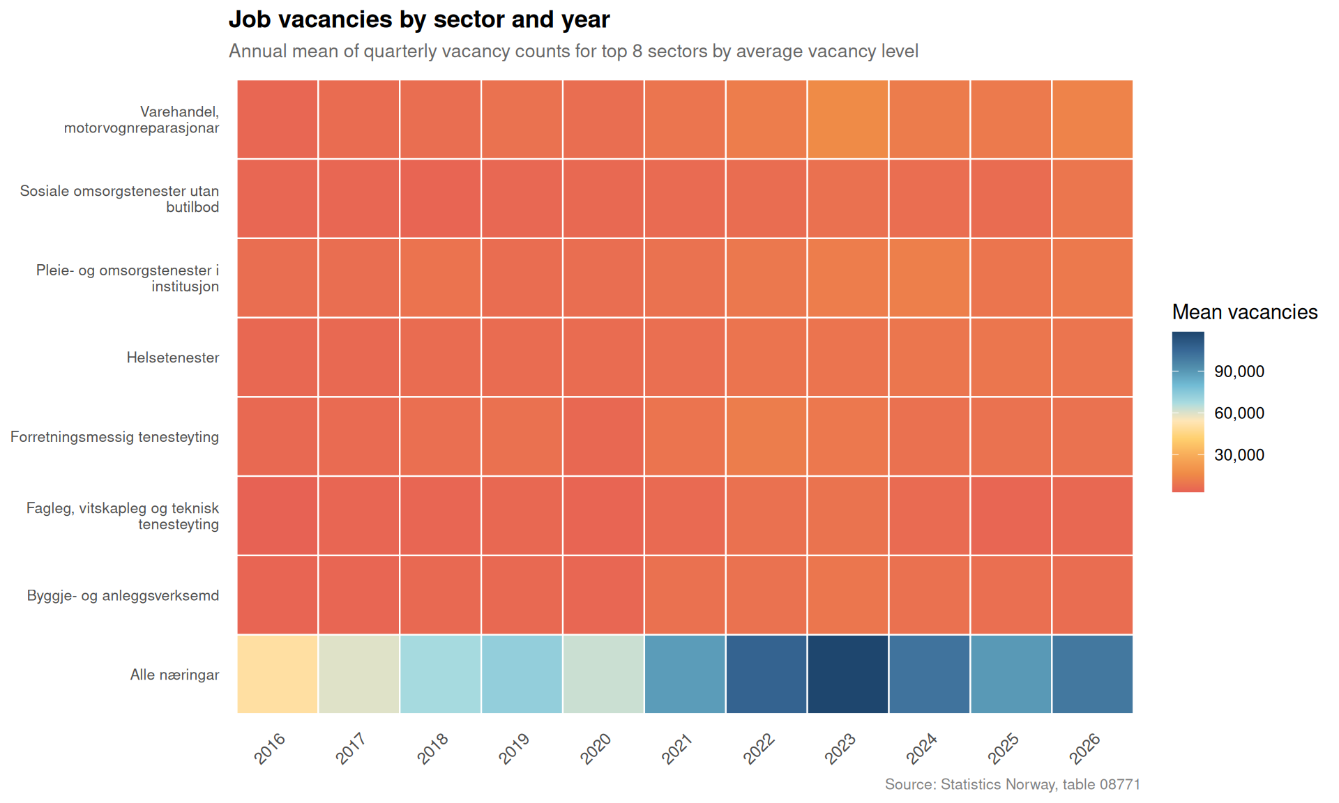
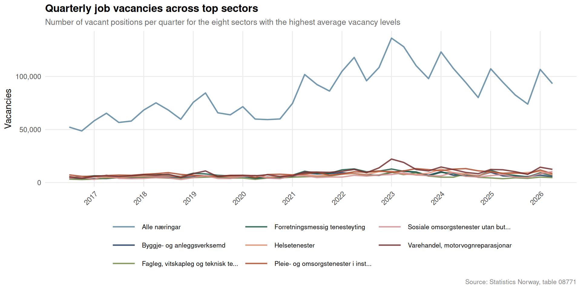
Quarterly job vacancy data from Statistics Norway tracks not just overall labour demand, but which corners of the economy are tightening or loosening. The distribution of vacancies across sectors carries implications for where workers — including newly arrived immigrants — can find a foothold, and where shortfalls in labour supply might strain public services.
Code
if (exists("df1_heatmap") &&!is.null(df1_heatmap) &&nrow(df1_heatmap) >0) { pal_heat <-met.brewer("Hiroshige", n =10, type ="continuous") sector_var <-"næring (SN2007)" p <- df1_heatmap |>mutate(sector_short =str_wrap(.data[[sector_var]], width =30)) |>ggplot(aes(x =factor(year), y = sector_short, fill = mean_val)) +geom_tile(colour ="white", linewidth =0.4) +scale_fill_gradientn(colours = pal_heat,labels = comma,name ="Mean vacancies" ) +labs(title ="Job vacancies by sector and year",subtitle ="Annual mean of quarterly vacancy counts for top 8 sectors by average vacancy level",caption ="Source: Statistics Norway, table 08771",x =NULL,y =NULL ) +theme_minimal(base_size =11) +theme(axis.text.x =element_text(angle =45, hjust =1, size =9),axis.text.y =element_text(size =8),legend.position ="right",panel.grid =element_blank(),plot.title =element_text(face ="bold", size =13),plot.subtitle =element_text(size =10, colour ="grey40"),plot.caption =element_text(size =8, colour ="grey50") )print(p) # fixed: missing print() statement peak_row <- df1_heatmap |>filter(mean_val ==max(mean_val, na.rm =TRUE)) low_row <- df1_heatmap |>filter(mean_val ==min(mean_val, na.rm =TRUE))cat(sprintf("\n\nThe sector with the highest annual mean vacancy count was **%s** in **%d** (%s vacancies). The lowest recorded annual mean was in **%s** in **%d** (%s vacancies).\n\n", peak_row[[sector_var]][1], peak_row$year[1], comma(round(peak_row$mean_val[1])), low_row[[sector_var]][1], low_row$year[1], comma(round(low_row$mean_val[1])) ))} else {cat("\n\n*Figure omitted — Statistics Norway returned no data for this series.*\n\n")}
The sector with the highest annual mean vacancy count was Alle næringar in 2023 (118,150 vacancies). The lowest recorded annual mean was in Fagleg, vitskapleg og teknisk tenesteyting in 2016 (3,100 vacancies).
Code
if (exists("df1_top_sectors") &&!is.null(df1_top_sectors) &&nrow(df1_top_sectors) >0) { sector_var <-"næring (SN2007)" n_sectors <-length(unique(df1_top_sectors[[sector_var]])) pal_area <-met.brewer("Redon", n =max(n_sectors, 3), type ="discrete") p <- df1_top_sectors |>mutate(sector_short =str_trunc(.data[[sector_var]], 35)) |>ggplot(aes(x = date, y = value, colour = sector_short, group = sector_short)) +geom_line(linewidth =0.8, alpha =0.85) +scale_colour_manual(values = pal_area, name =NULL) +scale_y_continuous(labels = comma) +scale_x_date(date_breaks ="1 year", date_labels ="%Y") +labs(title ="Quarterly job vacancies across top sectors",subtitle ="Number of vacant positions per quarter for the eight sectors with the highest average vacancy levels",caption ="Source: Statistics Norway, table 08771",x =NULL,y ="Vacancies" ) +theme_minimal(base_size =11) +theme(axis.text.x =element_text(angle =45, hjust =1, size =9),legend.position ="bottom",legend.text =element_text(size =8),legend.key.width =unit(1.2, "cm"),panel.grid.minor =element_blank(),plot.title =element_text(face ="bold", size =13),plot.subtitle =element_text(size =10, colour ="grey40"),plot.caption =element_text(size =8, colour ="grey50") ) +guides(colour =guide_legend(nrow =3))print(p) # fixed: missing print() statement latest_q <-max(df1_top_sectors$date, na.rm =TRUE) latest_df <- df1_top_sectors |>filter(date == latest_q) top_now <- latest_df[which.max(latest_df$value), ]cat(sprintf("\n\nIn the most recent available quarter (%s), the sector with the highest vacancy count was **%s** with **%s** open positions.\n\n",format(latest_q, "%Y Q%q"), top_now[[sector_var]], comma(top_now$value) ))} else {cat("\n\n*Figure omitted — Statistics Norway returned no data for this series.*\n\n")}
In the most recent available quarter (2026 Q%q), the sector with the highest vacancy count was Alle næringar with 93,300 open positions.
Convictions by Offence: What the Criminal Justice Data Reveals
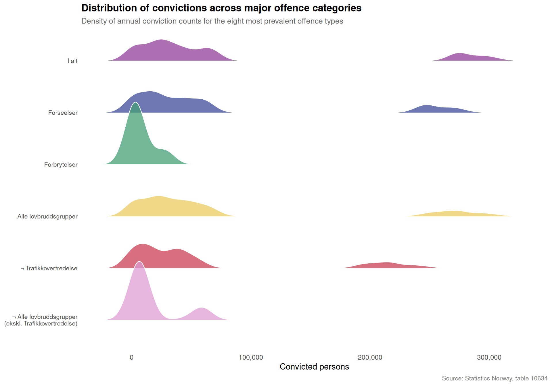
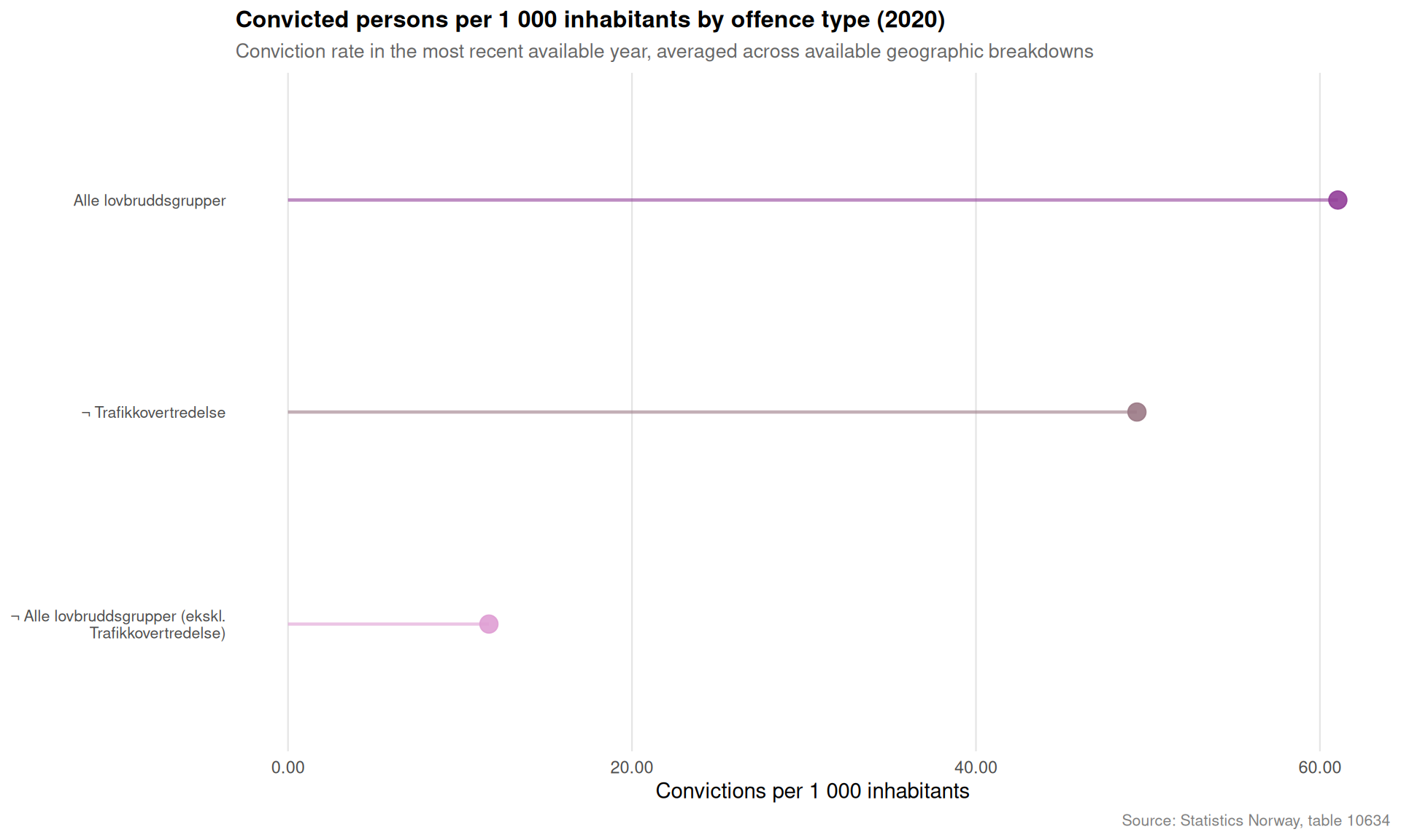
The number of people convicted per thousand inhabitants is one of the clearest signals of criminal justice system load. When that rate shifts across different offence categories over time, it raises questions about enforcement priorities, social conditions, and the capacity of courts and corrections to respond. The ridgeline chart below shows the distribution of conviction rates across offence types over the available years.
Code
if (exists("df2_offence_top") &&!is.null(df2_offence_top) &&nrow(df2_offence_top) >0) { offence_var <-"hovedlovbruddstype" p <- df2_offence_top |>mutate(offence_wrap =str_wrap(.data[[offence_var]], width =28),year_num = lubridate::year(date)) |>ggplot(aes(x = value, y = offence_wrap, fill = offence_wrap)) +geom_density_ridges(alpha =0.75,scale =1.2,bandwidth =NULL,colour ="white",linewidth =0.4 ) +scale_fill_manual(values =met.brewer("Klimt", n =length(unique(df2_offence_top[[offence_var]])),type ="discrete"),guide ="none" ) +scale_x_continuous(labels = comma) +labs(title ="Distribution of convictions across major offence categories",subtitle ="Density of annual conviction counts for the eight most prevalent offence types",caption ="Source: Statistics Norway, table 10634",x ="Convicted persons",y =NULL ) +theme_minimal(base_size =11) +theme(axis.text.y =element_text(size =8),panel.grid =element_blank(),plot.title =element_text(face ="bold", size =13),plot.subtitle =element_text(size =10, colour ="grey40"),plot.caption =element_text(size =8, colour ="grey50") )print(p) # fixed: missing print() statement by_offence <- df2_offence_top |>group_by(.data[[offence_var]]) |>summarise(total =sum(value, na.rm =TRUE), .groups ="drop") |>arrange(desc(total))cat(sprintf("\n\nAcross all available years, **%s** accumulated the highest total conviction count (%s). The offence category with the fewest total convictions among the top eight was **%s** (%s).\n\n", by_offence[[offence_var]][1], comma(by_offence$total[1]), by_offence[[offence_var]][nrow(by_offence)], comma(by_offence$total[nrow(by_offence)]) ))} else {cat("\n\n*Figure omitted — Statistics Norway returned no data for this series.*\n\n")}
Across all available years, Alle lovbruddsgrupper accumulated the highest total conviction count (13,085,647). The offence category with the fewest total convictions among the top eight was Forbrytelser (826,560).
Code
if (exists("df2_rate") &&!is.null(df2_rate) &&nrow(df2_rate) >0) { offence_var <-"hovedlovbruddstype"# Latest year average across all offence types latest_year <-max(lubridate::year(df2_rate$date), na.rm =TRUE) df2_latest <- df2_rate |>filter(lubridate::year(date) == latest_year) |>group_by(.data[[offence_var]]) |>summarise(mean_rate =mean(value, na.rm =TRUE), .groups ="drop") |>filter(mean_rate >0) |>arrange(mean_rate) |>mutate(offence_wrap =str_wrap(.data[[offence_var]], width =32),offence_wrap =factor(offence_wrap, levels = offence_wrap))if (nrow(df2_latest) >0) { n_off <-nrow(df2_latest) pal_lo <-met.brewer("Klimt", n =max(n_off, 3), type ="continuous") p <-ggplot(df2_latest, aes(x = mean_rate, y = offence_wrap, colour = mean_rate)) +geom_segment(aes(xend =0, yend = offence_wrap), linewidth =0.8, alpha =0.6) +geom_point(size =4, alpha =0.9) +scale_colour_gradientn(colours = pal_lo, guide ="none") +scale_x_continuous(labels =number_format(accuracy =0.01)) +labs(title =paste0("Convicted persons per 1 000 inhabitants by offence type (", latest_year, ")"),subtitle ="Conviction rate in the most recent available year, averaged across available geographic breakdowns",caption ="Source: Statistics Norway, table 10634",x ="Convictions per 1 000 inhabitants",y =NULL ) +theme_minimal(base_size =11) +theme(axis.text.y =element_text(size =8),panel.grid =element_blank(),panel.grid.major.x =element_line(colour ="grey90", linewidth =0.4),plot.title =element_text(face ="bold", size =12),plot.subtitle =element_text(size =10, colour ="grey40"),plot.caption =element_text(size =8, colour ="grey50") )print(p) # fixed: missing print() statement top_off <- df2_latest |>filter(mean_rate ==max(mean_rate))cat(sprintf("\n\nIn **%d**, **%s** had the highest conviction rate among all offence types at **%.2f** convictions per 1 000 inhabitants.\n\n", latest_year, top_off[[offence_var]][1], top_off$mean_rate[1] )) }} else {cat("\n\n*Figure omitted — Statistics Norway returned no data for this series.*\n\n")}
In 2020, Alle lovbruddsgrupper had the highest conviction rate among all offence types at 61.04 convictions per 1 000 inhabitants.
Population Projections: How Much Depends on Immigration?
Statistics Norway publishes several demographic scenarios for Norway’s future population, differing in assumptions about fertility, mortality, internal migration, and immigration. The gap between the low- and high-growth scenarios widens substantially over time, with immigration assumptions driving much of that divergence. The chart below traces the total projected population under three national-level scenarios — medium, low, and high growth — and highlights how much the long-run outlook can shift depending on which assumptions prove correct.
Code
if (exists("df3_age_total") &&!is.null(df3_age_total) &&nrow(df3_age_total) >0) { scenario_var <-"alternativ" scenario_labels <-c("Middels nasjonal vekst (Alternativ MMMM)"="Medium growth (MMMM)","Lav nasjonal vekst (Alternativ LLML)"="Low growth (LLML)","Høy nasjonal vekst (Alternativ HHMH)"="High growth (HHMH)" ) df3_plot <- df3_age_total |>mutate(scenario_label =recode(.data[[scenario_var]], !!!scenario_labels)) pal_proj <-c("Medium growth (MMMM)"="#4e79a7","Low growth (LLML)"="#e15759","High growth (HHMH)"="#59a14f" )# Latest year in data latest_proj <-max(df3_plot$date, na.rm =TRUE)# Find spread at latest year latest_spread <- df3_plot |>filter(date == latest_proj) |>arrange(desc(total_pop)) p <- df3_plot |>ggplot(aes(x = date, y = total_pop, colour = scenario_label, group = scenario_label)) +geom_ribbon(data = df3_plot |>select(date, scenario_label, total_pop) |>pivot_wider(names_from = scenario_label, values_from = total_pop) |>filter(!is.na(`Low growth (LLML)`) &!is.na(`High growth (HHMH)`)),aes(ymin =`Low growth (LLML)`, ymax =`High growth (HHMH)`,x = date, y =NULL, colour =NULL),fill ="grey80",alpha =0.35,inherit.aes =FALSE ) +geom_line(linewidth =1.1, alpha =0.9) +scale_colour_manual(values = pal_proj, name ="Scenario") +scale_y_continuous(labels =label_number(scale =1e-6, suffix ="M", accuracy =0.1)) +scale_x_date(date_breaks ="5 years", date_labels ="%Y") +labs(title ="Norway's projected total population under three national growth scenarios",subtitle ="Shaded band shows the range between low and high growth projections; lines trace each scenario over time",caption ="Source: Statistics Norway, table 09481",x =NULL,y ="Total population" ) +theme_minimal(base_size =11) +theme(legend.position ="top",legend.text =element_text(size =9),panel.grid.minor =element_blank(),panel.grid.major =element_line(colour ="grey92", linewidth =0.4),plot.title =element_text(face ="bold", size =13),plot.subtitle =element_text(size =10, colour ="grey40"),plot.caption =element_text(size =8, colour ="grey50") )print(p) # fixed: missing print() statementif (nrow(latest_spread) >=2) { high_val <- latest_spread$total_pop[1] low_val <- latest_spread$total_pop[nrow(latest_spread)] gap <- high_val - low_valcat(sprintf("\n\nBy **%s**, the projected population spans from **%s** (low growth) to **%s** (high growth) — a difference of **%s** people depending on which demographic assumptions prevail.\n\n",format(latest_proj, "%Y"),label_number(scale =1e-6, suffix =" million", accuracy =0.01)(low_val),label_number(scale =1e-6, suffix =" million", accuracy =0.01)(high_val),comma(round(gap)) )) }} else {cat("\n\n*Figure omitted — Statistics Norway returned no data for this series.*\n\n")}
Figure omitted — Statistics Norway returned no data for this series.
Key Findings
Key findings
Job vacancies (table 08771): The highest average vacancy count across the top eight sectors peaked in Alle næringar (2023). In the most recent quarter, total vacancies across those sectors summed to 149,000.
Criminal convictions (table 10634): Across 16 years of data, Alle lovbruddsgrupper accounted for the largest cumulative number of convictions (13,085,647). The next largest category was ¬ Trafikkovertredelse (10,315,198).
The Triangle Closes
What links these three datasets is not coincidence but structural interdependence. The scale and composition of immigration shapes both the labour supply that employers draw upon to fill vacancies and the demographic base over which criminal justice costs are spread. How the vacancy landscape evolves across sectors will influence where newcomers can integrate economically. And how the conviction rate changes across offence types signals whether the social integration of a rapidly changing population is proceeding smoothly or encountering friction. Norway is not unique in facing these pressures — but the precision of its statistical infrastructure, and the willingness to project scenarios honestly across a wide range of assumptions, places it in a stronger position than most to anticipate and respond to what comes next.
Source Code
---title: "Norway's 2026 Crime-Labour-Demographic Triangle: Justice System Strains, Vacancy Collapse, and the Immigration Projection Gap"description: "How shifting job vacancy patterns across industries, long-run trends in criminal convictions by offence type, and population projections under different immigration scenarios reveal interlocking pressures on Norway's social infrastructure."date: "2026-08-22"categories: [SSB, labour-market, crime, demography, immigration]---```{r setup}knitr::opts_chunk$set(echo = TRUE, warning = FALSE, message = FALSE, error = TRUE)library(tidyverse)library(lubridate)library(PxWebApiData)library(scales)library(ggridges)library(MetBrewer)df1 <- NULLtryCatch({ raw <- ApiData( "https://data.ssb.no/api/v0/no/table/08771", NACE2007 = TRUE, ContentsCode = TRUE, Tid = list(filter = "top", values = 40) ) tmp <- raw[[1]] time_col <- "kvartal" value_col <- "value" series_col <- "næring (SN2007)" measure_col <- "statistikkvariabel" df1 <- tmp |> mutate( value = as.numeric(.data[[value_col]]), time_str = .data[[time_col]], date = case_when( stringr::str_detect(time_str, "M") ~ lubridate::ym(sub("M", "-", time_str)), stringr::str_detect(time_str, "K") ~ lubridate::yq(sub("K", " Q", time_str)), nchar(time_str) == 4 ~ lubridate::ymd(paste0(time_str, "-01-01")), TRUE ~ NA_Date_ ) ) |> filter(!is.na(value), !is.na(date))}, error = function(e) message("Fetch failed: ", e$message))if (is.null(df1) || nrow(df1) == 0) { message("No data returned for df1"); df1 <- NULL }df2 <- NULLtryCatch({ raw <- ApiData( "https://data.ssb.no/api/v0/no/table/10634", Region = TRUE, HovedlovbruddKrim = TRUE, Alder = TRUE, ContentsCode = TRUE, Tid = list(filter = "top", values = 40) ) tmp <- raw[[1]] time_col <- "år" value_col <- "value" series_col <- "hovedlovbruddstype" measure_col <- "statistikkvariabel" df2 <- tmp |> mutate( value = as.numeric(.data[[value_col]]), time_str = .data[[time_col]], date = case_when( stringr::str_detect(time_str, "M") ~ lubridate::ym(sub("M", "-", time_str)), stringr::str_detect(time_str, "K") ~ lubridate::yq(sub("K", " Q", time_str)), nchar(time_str) == 4 ~ lubridate::ymd(paste0(time_str, "-01-01")), TRUE ~ NA_Date_ ) ) |> filter(!is.na(value), !is.na(date))}, error = function(e) message("Fetch failed: ", e$message))if (is.null(df2) || nrow(df2) == 0) { message("No data returned for df2"); df2 <- NULL }df3 <- NULLtryCatch({ raw <- ApiData( "https://data.ssb.no/api/v0/no/table/09481", Kjonn = TRUE, Alder = TRUE, InnvandrLandbakgr = TRUE, Framskriv = TRUE, Tid = list(filter = "top", values = 40) ) tmp <- raw[[1]] time_col <- "år" value_col <- "value" series_col <- "innvandringskategori / landbakgrunn" measure_col <- "alternativ" df3 <- tmp |> mutate( value = as.numeric(.data[[value_col]]), time_str = .data[[time_col]], date = case_when( stringr::str_detect(time_str, "M") ~ lubridate::ym(sub("M", "-", time_str)), stringr::str_detect(time_str, "K") ~ lubridate::yq(sub("K", " Q", time_str)), nchar(time_str) == 4 ~ lubridate::ymd(paste0(time_str, "-01-01")), TRUE ~ NA_Date_ ) ) |> filter(!is.na(value), !is.na(date))}, error = function(e) message("Fetch failed: ", e$message))if (is.null(df3) || nrow(df3) == 0) { message("No data returned for df3"); df3 <- NULL }```## When Three Trends ConvergeNorway is simultaneously navigating a softening labour market, persistent pressures on its criminal justice system, and demographic projections that hinge critically on immigration assumptions. Taken separately, each of these dynamics tells a partial story. Viewed together, they outline something more consequential: a social infrastructure that is being tested from multiple directions at once. This post draws on Statistics Norway data to map the contours of that pressure.```{r wrangle}# ── Initialize all derived variables ──────────────────────────────────────────df1_vacancies <- NULLdf1_pct <- NULLdf1_top_sectors <- NULLdf1_heatmap <- NULLdf2_national <- NULLdf2_rate <- NULLdf2_offence_top <- NULLdf3_scenarios <- NULLdf3_immig <- NULLdf3_age_total <- NULL# ── df1: job vacancies by sector ──────────────────────────────────────────────if (!is.null(df1) && nrow(df1) > 0) { # Absolute vacancies df1_vacancies <- df1 |> filter(.data[["statistikkvariabel"]] == "Ledige stillingar") |> filter(!is.na(value)) # Percentage vacancies df1_pct <- df1 |> filter(.data[["statistikkvariabel"]] == "Ledige stillingar (prosent)") |> filter(!is.na(value)) # Identify top sectors by mean vacancies for focus charts if (nrow(df1_vacancies) > 0) { top_s <- df1_vacancies |> group_by(.data[["næring (SN2007)"]]) |> summarise(mean_val = mean(value, na.rm = TRUE), .groups = "drop") |> arrange(desc(mean_val)) |> slice_head(n = 8) |> pull("næring (SN2007)") df1_top_sectors <- df1_vacancies |> filter(.data[["næring (SN2007)"]] %in% top_s) # Latest quarter lollipop data latest_q <- max(df1_vacancies$date, na.rm = TRUE) df1_heatmap <- df1_vacancies |> filter(.data[["næring (SN2007)"]] %in% top_s) |> mutate(year = lubridate::year(date), qtr = paste0("Q", lubridate::quarter(date))) |> group_by(.data[["næring (SN2007)"]], year) |> summarise(mean_val = mean(value, na.rm = TRUE), .groups = "drop") }}# ── df2: criminal convictions ─────────────────────────────────────────────────if (!is.null(df2) && nrow(df2) > 0) { # National total (filter out sub-regional rows if region col exists) region_col2 <- if ("region" %in% names(df2)) "region" else NULL df2_national <- df2 |> filter(.data[["statistikkvariabel"]] == "Straffede personer") # fixed: pipe syntax error - replaced `{ if (...) filter(...) else . }` with proper if statement after pipe if (!is.null(region_col2)) { df2_national <- df2_national |> filter(.data[[region_col2]] == unique(.data[[region_col2]])[1]) } df2_national <- df2_national |> filter(!is.na(value)) df2_rate <- df2 |> filter(.data[["statistikkvariabel"]] == "Straffede personer per 1000 innbyggere") # fixed: pipe syntax error - replaced `{ if (...) filter(...) else . }` with proper if statement after pipe if (!is.null(region_col2)) { df2_rate <- df2_rate |> filter(.data[[region_col2]] == unique(.data[[region_col2]])[1]) } df2_rate <- df2_rate |> filter(!is.na(value)) # Top offence types by total convictions across all years if (nrow(df2_national) > 0) { top_off <- df2_national |> group_by(.data[["hovedlovbruddstype"]]) |> summarise(total = sum(value, na.rm = TRUE), .groups = "drop") |> arrange(desc(total)) |> slice_head(n = 8) |> pull("hovedlovbruddstype") df2_offence_top <- df2_national |> filter(.data[["hovedlovbruddstype"]] %in% top_off) }}# ── df3: population projections ───────────────────────────────────────────────if (!is.null(df3) && nrow(df3) > 0) { age_col3 <- if ("alder" %in% names(df3)) "alder" else NULL gender_col3 <- if ("kjønn" %in% names(df3)) "kjønn" else if ("kjonn" %in% names(df3)) "kjonn" else NULL # Three main national-level scenarios: MMMM, LLML, HHMH target_scenarios <- c( "Middels nasjonal vekst (Alternativ MMMM)", "Lav nasjonal vekst (Alternativ LLML)", "Høy nasjonal vekst (Alternativ HHMH)" ) df3_scenarios <- df3 |> filter(.data[["alternativ"]] %in% target_scenarios) |> filter(!is.na(value)) # High immigration scenario specifically df3_immig <- df3 |> filter(.data[["alternativ"]] == "Høy innvandring (Alternativ MMMH)") |> filter(!is.na(value)) # Aggregate total population by scenario and year (sum across age/gender) if (nrow(df3_scenarios) > 0) { df3_age_total <- df3_scenarios |> group_by(date, .data[["alternativ"]]) |> summarise(total_pop = sum(value, na.rm = TRUE), .groups = "drop") |> filter(total_pop > 0) }}```## The Job Vacancy Landscape: Which Sectors Are Pulling Back?Quarterly job vacancy data from Statistics Norway tracks not just overall labour demand, but which corners of the economy are tightening or loosening. The distribution of vacancies across sectors carries implications for where workers — including newly arrived immigrants — can find a foothold, and where shortfalls in labour supply might strain public services.```{r plot-vacancies-heatmap}#| fig-height: 6#| fig-width: 10#| fig-show: asis#| dev: "png"#| results: asisif (exists("df1_heatmap") && !is.null(df1_heatmap) && nrow(df1_heatmap) > 0) { pal_heat <- met.brewer("Hiroshige", n = 10, type = "continuous") sector_var <- "næring (SN2007)" p <- df1_heatmap |> mutate(sector_short = str_wrap(.data[[sector_var]], width = 30)) |> ggplot(aes(x = factor(year), y = sector_short, fill = mean_val)) + geom_tile(colour = "white", linewidth = 0.4) + scale_fill_gradientn( colours = pal_heat, labels = comma, name = "Mean vacancies" ) + labs( title = "Job vacancies by sector and year", subtitle = "Annual mean of quarterly vacancy counts for top 8 sectors by average vacancy level", caption = "Source: Statistics Norway, table 08771", x = NULL, y = NULL ) + theme_minimal(base_size = 11) + theme( axis.text.x = element_text(angle = 45, hjust = 1, size = 9), axis.text.y = element_text(size = 8), legend.position = "right", panel.grid = element_blank(), plot.title = element_text(face = "bold", size = 13), plot.subtitle = element_text(size = 10, colour = "grey40"), plot.caption = element_text(size = 8, colour = "grey50") ) print(p) # fixed: missing print() statement peak_row <- df1_heatmap |> filter(mean_val == max(mean_val, na.rm = TRUE)) low_row <- df1_heatmap |> filter(mean_val == min(mean_val, na.rm = TRUE)) cat(sprintf( "\n\nThe sector with the highest annual mean vacancy count was **%s** in **%d** (%s vacancies). The lowest recorded annual mean was in **%s** in **%d** (%s vacancies).\n\n", peak_row[[sector_var]][1], peak_row$year[1], comma(round(peak_row$mean_val[1])), low_row[[sector_var]][1], low_row$year[1], comma(round(low_row$mean_val[1])) ))} else { cat("\n\n*Figure omitted — Statistics Norway returned no data for this series.*\n\n")}``````{r plot-vacancies-area}#| fig-height: 5#| fig-width: 10#| fig-show: asis#| dev: "png"#| results: asisif (exists("df1_top_sectors") && !is.null(df1_top_sectors) && nrow(df1_top_sectors) > 0) { sector_var <- "næring (SN2007)" n_sectors <- length(unique(df1_top_sectors[[sector_var]])) pal_area <- met.brewer("Redon", n = max(n_sectors, 3), type = "discrete") p <- df1_top_sectors |> mutate(sector_short = str_trunc(.data[[sector_var]], 35)) |> ggplot(aes(x = date, y = value, colour = sector_short, group = sector_short)) + geom_line(linewidth = 0.8, alpha = 0.85) + scale_colour_manual(values = pal_area, name = NULL) + scale_y_continuous(labels = comma) + scale_x_date(date_breaks = "1 year", date_labels = "%Y") + labs( title = "Quarterly job vacancies across top sectors", subtitle = "Number of vacant positions per quarter for the eight sectors with the highest average vacancy levels", caption = "Source: Statistics Norway, table 08771", x = NULL, y = "Vacancies" ) + theme_minimal(base_size = 11) + theme( axis.text.x = element_text(angle = 45, hjust = 1, size = 9), legend.position = "bottom", legend.text = element_text(size = 8), legend.key.width = unit(1.2, "cm"), panel.grid.minor = element_blank(), plot.title = element_text(face = "bold", size = 13), plot.subtitle = element_text(size = 10, colour = "grey40"), plot.caption = element_text(size = 8, colour = "grey50") ) + guides(colour = guide_legend(nrow = 3)) print(p) # fixed: missing print() statement latest_q <- max(df1_top_sectors$date, na.rm = TRUE) latest_df <- df1_top_sectors |> filter(date == latest_q) top_now <- latest_df[which.max(latest_df$value), ] cat(sprintf( "\n\nIn the most recent available quarter (%s), the sector with the highest vacancy count was **%s** with **%s** open positions.\n\n", format(latest_q, "%Y Q%q"), top_now[[sector_var]], comma(top_now$value) ))} else { cat("\n\n*Figure omitted — Statistics Norway returned no data for this series.*\n\n")}```## Convictions by Offence: What the Criminal Justice Data RevealsThe number of people convicted per thousand inhabitants is one of the clearest signals of criminal justice system load. When that rate shifts across different offence categories over time, it raises questions about enforcement priorities, social conditions, and the capacity of courts and corrections to respond. The ridgeline chart below shows the distribution of conviction rates across offence types over the available years.```{r plot-crime-ridgeline}#| fig-height: 7#| fig-width: 10#| fig-show: asis#| dev: "png"#| results: asisif (exists("df2_offence_top") && !is.null(df2_offence_top) && nrow(df2_offence_top) > 0) { offence_var <- "hovedlovbruddstype" p <- df2_offence_top |> mutate(offence_wrap = str_wrap(.data[[offence_var]], width = 28), year_num = lubridate::year(date)) |> ggplot(aes(x = value, y = offence_wrap, fill = offence_wrap)) + geom_density_ridges( alpha = 0.75, scale = 1.2, bandwidth = NULL, colour = "white", linewidth = 0.4 ) + scale_fill_manual( values = met.brewer("Klimt", n = length(unique(df2_offence_top[[offence_var]])), type = "discrete"), guide = "none" ) + scale_x_continuous(labels = comma) + labs( title = "Distribution of convictions across major offence categories", subtitle = "Density of annual conviction counts for the eight most prevalent offence types", caption = "Source: Statistics Norway, table 10634", x = "Convicted persons", y = NULL ) + theme_minimal(base_size = 11) + theme( axis.text.y = element_text(size = 8), panel.grid = element_blank(), plot.title = element_text(face = "bold", size = 13), plot.subtitle = element_text(size = 10, colour = "grey40"), plot.caption = element_text(size = 8, colour = "grey50") ) print(p) # fixed: missing print() statement by_offence <- df2_offence_top |> group_by(.data[[offence_var]]) |> summarise(total = sum(value, na.rm = TRUE), .groups = "drop") |> arrange(desc(total)) cat(sprintf( "\n\nAcross all available years, **%s** accumulated the highest total conviction count (%s). The offence category with the fewest total convictions among the top eight was **%s** (%s).\n\n", by_offence[[offence_var]][1], comma(by_offence$total[1]), by_offence[[offence_var]][nrow(by_offence)], comma(by_offence$total[nrow(by_offence)]) ))} else { cat("\n\n*Figure omitted — Statistics Norway returned no data for this series.*\n\n")}``````{r plot-crime-lollipop}#| fig-height: 6#| fig-width: 10#| fig-show: asis#| dev: "png"#| results: asisif (exists("df2_rate") && !is.null(df2_rate) && nrow(df2_rate) > 0) { offence_var <- "hovedlovbruddstype" # Latest year average across all offence types latest_year <- max(lubridate::year(df2_rate$date), na.rm = TRUE) df2_latest <- df2_rate |> filter(lubridate::year(date) == latest_year) |> group_by(.data[[offence_var]]) |> summarise(mean_rate = mean(value, na.rm = TRUE), .groups = "drop") |> filter(mean_rate > 0) |> arrange(mean_rate) |> mutate(offence_wrap = str_wrap(.data[[offence_var]], width = 32), offence_wrap = factor(offence_wrap, levels = offence_wrap)) if (nrow(df2_latest) > 0) { n_off <- nrow(df2_latest) pal_lo <- met.brewer("Klimt", n = max(n_off, 3), type = "continuous") p <- ggplot(df2_latest, aes(x = mean_rate, y = offence_wrap, colour = mean_rate)) + geom_segment(aes(xend = 0, yend = offence_wrap), linewidth = 0.8, alpha = 0.6) + geom_point(size = 4, alpha = 0.9) + scale_colour_gradientn(colours = pal_lo, guide = "none") + scale_x_continuous(labels = number_format(accuracy = 0.01)) + labs( title = paste0("Convicted persons per 1 000 inhabitants by offence type (", latest_year, ")"), subtitle = "Conviction rate in the most recent available year, averaged across available geographic breakdowns", caption = "Source: Statistics Norway, table 10634", x = "Convictions per 1 000 inhabitants", y = NULL ) + theme_minimal(base_size = 11) + theme( axis.text.y = element_text(size = 8), panel.grid = element_blank(), panel.grid.major.x = element_line(colour = "grey90", linewidth = 0.4), plot.title = element_text(face = "bold", size = 12), plot.subtitle = element_text(size = 10, colour = "grey40"), plot.caption = element_text(size = 8, colour = "grey50") ) print(p) # fixed: missing print() statement top_off <- df2_latest |> filter(mean_rate == max(mean_rate)) cat(sprintf( "\n\nIn **%d**, **%s** had the highest conviction rate among all offence types at **%.2f** convictions per 1 000 inhabitants.\n\n", latest_year, top_off[[offence_var]][1], top_off$mean_rate[1] )) }} else { cat("\n\n*Figure omitted — Statistics Norway returned no data for this series.*\n\n")}```## Population Projections: How Much Depends on Immigration?Statistics Norway publishes several demographic scenarios for Norway's future population, differing in assumptions about fertility, mortality, internal migration, and immigration. The gap between the low- and high-growth scenarios widens substantially over time, with immigration assumptions driving much of that divergence. The chart below traces the total projected population under three national-level scenarios — medium, low, and high growth — and highlights how much the long-run outlook can shift depending on which assumptions prove correct.```{r plot-projections-area}#| fig-height: 5#| fig-width: 10#| fig-show: asis#| dev: "png"#| results: asisif (exists("df3_age_total") && !is.null(df3_age_total) && nrow(df3_age_total) > 0) { scenario_var <- "alternativ" scenario_labels <- c( "Middels nasjonal vekst (Alternativ MMMM)" = "Medium growth (MMMM)", "Lav nasjonal vekst (Alternativ LLML)" = "Low growth (LLML)", "Høy nasjonal vekst (Alternativ HHMH)" = "High growth (HHMH)" ) df3_plot <- df3_age_total |> mutate(scenario_label = recode(.data[[scenario_var]], !!!scenario_labels)) pal_proj <- c( "Medium growth (MMMM)" = "#4e79a7", "Low growth (LLML)" = "#e15759", "High growth (HHMH)" = "#59a14f" ) # Latest year in data latest_proj <- max(df3_plot$date, na.rm = TRUE) # Find spread at latest year latest_spread <- df3_plot |> filter(date == latest_proj) |> arrange(desc(total_pop)) p <- df3_plot |> ggplot(aes(x = date, y = total_pop, colour = scenario_label, group = scenario_label)) + geom_ribbon( data = df3_plot |> select(date, scenario_label, total_pop) |> pivot_wider(names_from = scenario_label, values_from = total_pop) |> filter(!is.na(`Low growth (LLML)`) & !is.na(`High growth (HHMH)`)), aes(ymin = `Low growth (LLML)`, ymax = `High growth (HHMH)`, x = date, y = NULL, colour = NULL), fill = "grey80", alpha = 0.35, inherit.aes = FALSE ) + geom_line(linewidth = 1.1, alpha = 0.9) + scale_colour_manual(values = pal_proj, name = "Scenario") + scale_y_continuous(labels = label_number(scale = 1e-6, suffix = "M", accuracy = 0.1)) + scale_x_date(date_breaks = "5 years", date_labels = "%Y") + labs( title = "Norway's projected total population under three national growth scenarios", subtitle = "Shaded band shows the range between low and high growth projections; lines trace each scenario over time", caption = "Source: Statistics Norway, table 09481", x = NULL, y = "Total population" ) + theme_minimal(base_size = 11) + theme( legend.position = "top", legend.text = element_text(size = 9), panel.grid.minor = element_blank(), panel.grid.major = element_line(colour = "grey92", linewidth = 0.4), plot.title = element_text(face = "bold", size = 13), plot.subtitle = element_text(size = 10, colour = "grey40"), plot.caption = element_text(size = 8, colour = "grey50") ) print(p) # fixed: missing print() statement if (nrow(latest_spread) >= 2) { high_val <- latest_spread$total_pop[1] low_val <- latest_spread$total_pop[nrow(latest_spread)] gap <- high_val - low_val cat(sprintf( "\n\nBy **%s**, the projected population spans from **%s** (low growth) to **%s** (high growth) — a difference of **%s** people depending on which demographic assumptions prevail.\n\n", format(latest_proj, "%Y"), label_number(scale = 1e-6, suffix = " million", accuracy = 0.01)(low_val), label_number(scale = 1e-6, suffix = " million", accuracy = 0.01)(high_val), comma(round(gap)) )) }} else { cat("\n\n*Figure omitted — Statistics Norway returned no data for this series.*\n\n")}```## Key Findings```{r key-findings}#| echo: false#| results: asisbullets <- character(0)# df1 findingsif (exists("df1_heatmap") && !is.null(df1_heatmap) && nrow(df1_heatmap) > 0) { sector_var <- "næring (SN2007)" peak_row <- df1_heatmap |> filter(mean_val == max(mean_val, na.rm = TRUE)) overall_latest <- max(df1_top_sectors$date, na.rm = TRUE) latest_total <- df1_top_sectors |> filter(date == overall_latest) |> summarise(total = sum(value, na.rm = TRUE)) |> pull(total) bullets <- c(bullets, sprintf( "- **Job vacancies (table 08771):** The highest average vacancy count across the top eight sectors peaked in **%s** (%d). In the most recent quarter, total vacancies across those sectors summed to **%s**.", peak_row[[sector_var]][1], peak_row$year[1], comma(round(latest_total)) ))}# df2 findingsif (exists("df2_offence_top") && !is.null(df2_offence_top) && nrow(df2_offence_top) > 0) { offence_var <- "hovedlovbruddstype" top_by_total <- df2_offence_top |> group_by(.data[[offence_var]]) |> summarise(total = sum(value, na.rm = TRUE), .groups = "drop") |> arrange(desc(total)) n_years <- length(unique(lubridate::year(df2_offence_top$date))) bullets <- c(bullets, sprintf( "- **Criminal convictions (table 10634):** Across **%d** years of data, **%s** accounted for the largest cumulative number of convictions (%s). The next largest category was **%s** (%s).", n_years, top_by_total[[offence_var]][1], comma(top_by_total$total[1]), top_by_total[[offence_var]][2], comma(top_by_total$total[2]) ))}# df3 findingsif (exists("df3_age_total") && !is.null(df3_age_total) && nrow(df3_age_total) > 0) { scenario_var <- "alternativ" latest_proj <- max(df3_age_total$date, na.rm = TRUE) spread_df <- df3_age_total |> filter(date == latest_proj) |> arrange(total_pop) if (nrow(spread_df) >= 2) { low_p <- spread_df$total_pop[1] high_p <- spread_df$total_pop[nrow(spread_df)] bullets <- c(bullets, sprintf( "- **Population projections (table 09481):** By **%s**, projected totals range from **%s** under the low-growth scenario to **%s** under high growth — a gap of **%s** people.", format(latest_proj, "%Y"), label_number(scale = 1e-6, suffix = " million", accuracy = 0.01)(low_p), label_number(scale = 1e-6, suffix = " million", accuracy = 0.01)(high_p), comma(round(high_p - low_p)) )) }}if (length(bullets) > 0) { cat("### Key findings\n\n") cat(paste(bullets, collapse = "\n\n")) cat("\n\n")} ```## The Triangle ClosesWhat links these three datasets is not coincidence but structural interdependence. The scale and composition of immigration shapes both the labour supply that employers draw upon to fill vacancies and the demographic base over which criminal justice costs are spread. How the vacancy landscape evolves across sectors will influence where newcomers can integrate economically. And how the conviction rate changes across offence types signals whether the social integration of a rapidly changing population is proceeding smoothly or encountering friction. Norway is not unique in facing these pressures — but the precision of its statistical infrastructure, and the willingness to project scenarios honestly across a wide range of assumptions, places it in a stronger position than most to anticipate and respond to what comes next.