How export weakness, persistent smoking rates, and shifting citizenship patterns reveal structural tensions beneath Norway’s prosperity narrative.
Published
August 18, 2026
Norway presents a puzzle to outside observers: a wealthy, well-governed nation with world-class public services, yet one facing simultaneous pressures on its export base, its population health outcomes, and its demographic sustainability. This post draws on Statistics Norway data covering trade flows, smoking prevalence by age and gender, and population by citizenship to map three structural fault lines that official GDP figures tend to obscure.
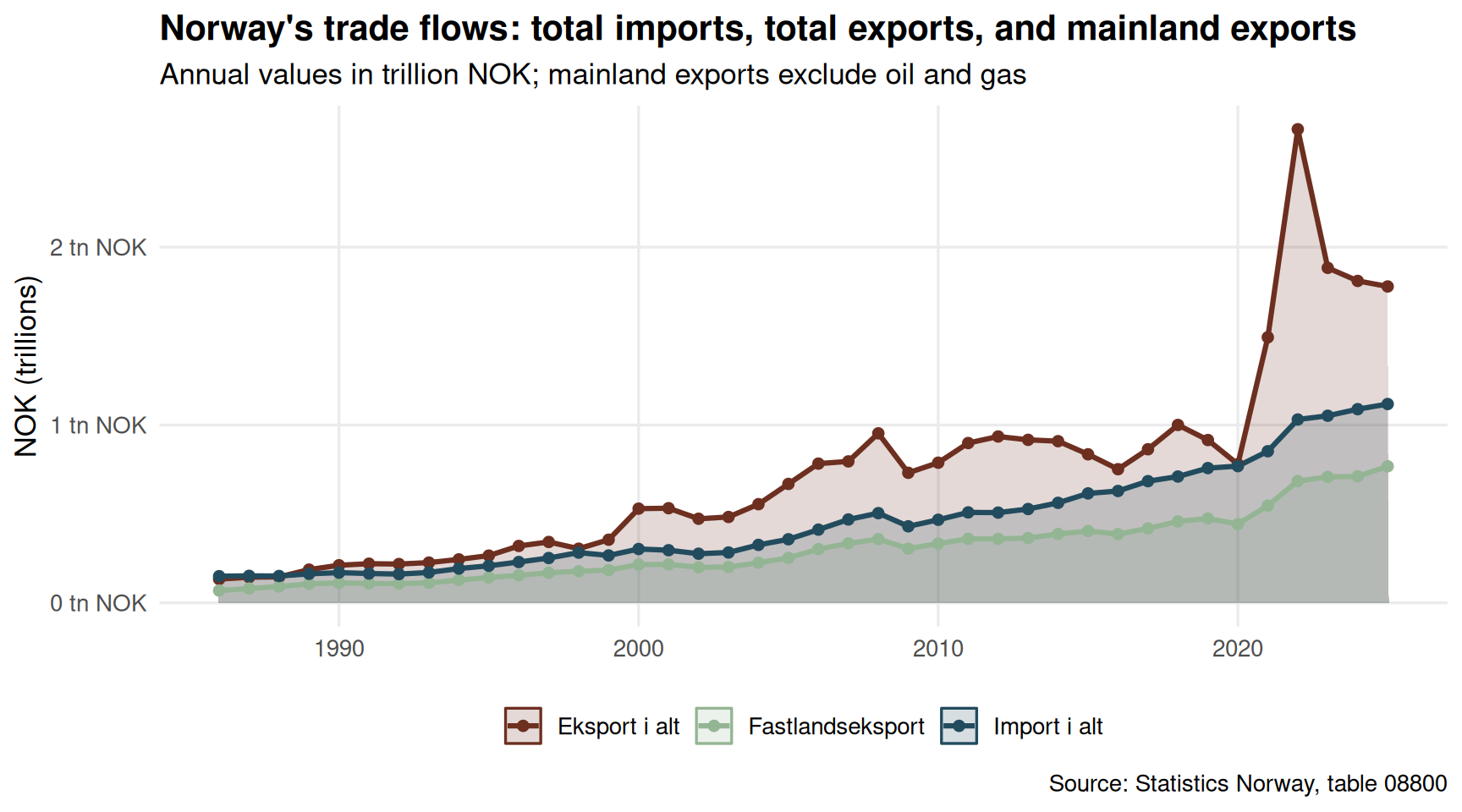
Norway’s total export figures have long been dominated by petroleum. But the mainland export component — goods produced onshore and sold abroad — tells a different story about the competitiveness of Norway’s non-oil economy. How has this evolved alongside the overall trade balance?
Code
if (exists("df1_trade") &&!is.null(df1_trade) &&nrow(df1_trade) >0) { pal <- MetBrewer::met.brewer("Hokusai1", n =3) p <-ggplot(df1_trade, aes(x = year, y = value /1e6, colour = label, fill = label)) +geom_area(alpha =0.18, position ="identity") +geom_line(linewidth =1.1) +geom_point(size =1.8) +scale_colour_manual(values = pal, name =NULL) +scale_fill_manual(values = pal, name =NULL) +scale_y_continuous(labels = scales::label_comma(suffix =" tn NOK")) +scale_x_continuous(breaks = scales::pretty_breaks()) +labs(title ="Norway's trade flows: total imports, total exports, and mainland exports",subtitle ="Annual values in trillion NOK; mainland exports exclude oil and gas",caption ="Source: Statistics Norway, table 08800",x =NULL, y ="NOK (trillions)" ) +theme_minimal(base_size =13) +theme(legend.position ="bottom",panel.grid.minor =element_blank(),plot.title =element_text(face ="bold") )print(p) latest_yr <-max(df1_trade$year) mainland <- df1_trade |>filter(year == latest_yr, label =="Fastlandseksport") total_exp <- df1_trade |>filter(year == latest_yr, label =="Eksport i alt") total_imp <- df1_trade |>filter(year == latest_yr, label =="Import i alt")if (nrow(mainland) >0&&nrow(total_exp) >0) { share <- mainland$value / total_exp$value *100cat(sprintf("\n\nIn %d, mainland exports accounted for %.1f%% of total exports (%.2f trillion NOK out of %.2f trillion NOK).\n\n", latest_yr, share, mainland$value /1e6, total_exp$value /1e6 )) }} else {cat("\n\n*Figure omitted — Statistics Norway returned no data for this series.*\n\n")}
In 2025, mainland exports accounted for 43.2% of total exports (0.77 trillion NOK out of 1.78 trillion NOK).
Code
if (exists("df1_waterfall") &&!is.null(df1_waterfall) &&nrow(df1_waterfall) >0) { pal2 <-c("TRUE"="#4a7c59", "FALSE"="#c0392b") p2 <-ggplot(df1_waterfall, aes(x =factor(year), y = change /1e6, fill = positive)) +geom_col(width =0.65, colour ="white", linewidth =0.3) +geom_hline(yintercept =0, colour ="grey30", linewidth =0.5) +geom_text(aes(label =sprintf("%+.0f", change /1e6),vjust =ifelse(change >=0, -0.4, 1.3) ),size =3.4, fontface ="bold",colour =ifelse(df1_waterfall$positive, "#4a7c59", "#c0392b") ) +scale_fill_manual(values = pal2, guide ="none") +scale_y_continuous(labels = scales::label_comma(suffix =" tn NOK")) +labs(title ="Year-on-year change in Norway's merchandise trade balance",subtitle ="Bars show absolute NOK change from previous year; green = improvement, red = deterioration",caption ="Source: Statistics Norway, table 08800",x =NULL, y ="Change (trillion NOK)" ) +theme_minimal(base_size =13) +theme(panel.grid.minor =element_blank(),panel.grid.major.x =element_blank(),plot.title =element_text(face ="bold") )print(p2) worst_yr <- df1_waterfall[which.min(df1_waterfall$change), ] best_yr <- df1_waterfall[which.max(df1_waterfall$change), ]cat(sprintf("\n\nThe sharpest single-year deterioration in the trade balance occurred in %d (%.2f trillion NOK change), while the strongest improvement came in %d (+%.2f trillion NOK).\n\n", worst_yr$year, worst_yr$change /1e6, best_yr$year, best_yr$change /1e6 ))} else {cat("\n\n*Figure omitted — Statistics Norway returned no data for this series.*\n\n")}
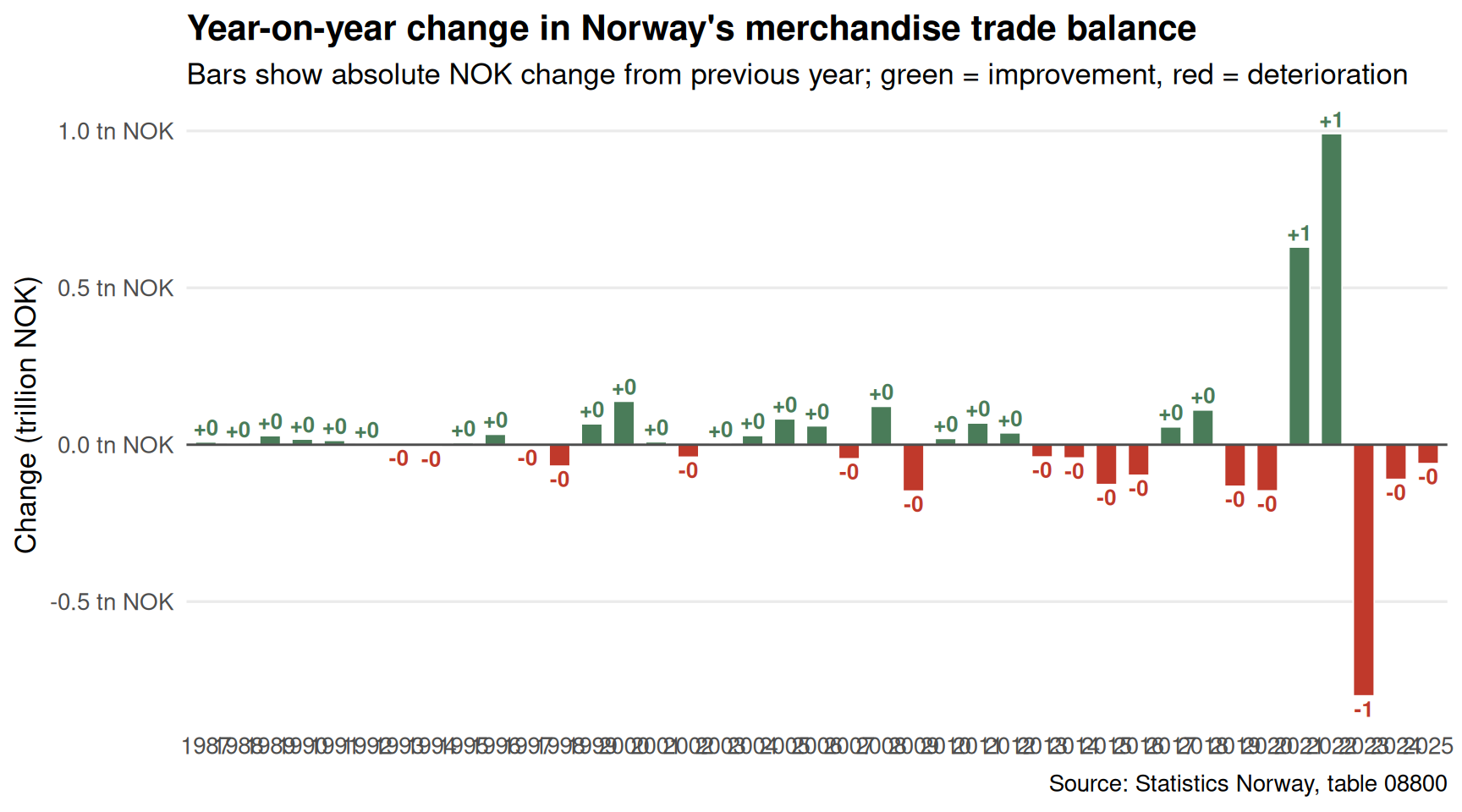
The sharpest single-year deterioration in the trade balance occurred in 2023 (-0.80 trillion NOK change), while the strongest improvement came in 2022 (+0.99 trillion NOK).
Public Health: Smoking Rates by Age and Gender
Norway has reduced smoking substantially over recent decades, but the pace of decline has not been uniform across age groups. Data from SSB’s health survey (table 05307) capture both daily and occasional smoking prevalence — together painting a picture of where residual tobacco use is concentrated.
Code
if (exists("df2_age") &&!is.null(df2_age) &&nrow(df2_age) >0) {# Need enough years for ridgeline to make sense n_years <-length(unique(df2_age$year))if (n_years >=3) { pal3 <- MetBrewer::met.brewer("Hiroshige", n = n_years) p3 <-ggplot(df2_age,aes(x = value, y =reorder(age_group, value, FUN = mean),fill =factor(year))) + ggridges::geom_density_ridges(alpha =0.65, scale =1.4,bandwidth =1.5, colour ="white", linewidth =0.4 ) +scale_fill_manual(values = pal3, name ="Year") +scale_x_continuous(labels = scales::label_number(suffix ="%")) +labs(title ="Distribution of daily smoking rates across age groups",subtitle ="Each ridge shows the spread of prevalence estimates by age group; values in percent",caption ="Source: Statistics Norway, table 05307",x ="Daily smokers (%)", y =NULL ) +theme_minimal(base_size =13) +theme(legend.position ="right",panel.grid.minor =element_blank(),plot.title =element_text(face ="bold") )print(p3) highest_age <- df2_age |>group_by(age_group) |>summarise(mean_val =mean(value, na.rm =TRUE)) |>slice_max(mean_val, n =1)cat(sprintf("\n\nAmong the age groups tracked, '%s' recorded the highest average daily smoking prevalence (%.1f%% on average across years).\n\n", highest_age$age_group, highest_age$mean_val )) } else {# Fallback lollipop if too few years for ridgeline latest_smoke_yr <-max(df2_age$year) df2_age_latest <- df2_age |>filter(year == latest_smoke_yr)if (!is.null(df2_age_latest) &&nrow(df2_age_latest) >0) { p3b <-ggplot(df2_age_latest,aes(x = value, y =reorder(age_group, value))) +geom_segment(aes(xend =0, yend =reorder(age_group, value)),colour ="grey70", linewidth =0.7) +geom_point(colour ="#3d6b8e", size =4) +geom_text(aes(label =sprintf("%.1f%%", value)),hjust =-0.3, size =3.5) +scale_x_continuous(labels = scales::label_number(suffix ="%"),expand =expansion(mult =c(0, 0.15))) +labs(title =sprintf("Daily smoking prevalence by age group, %d", latest_smoke_yr),subtitle ="Percentage of daily smokers within each age group",caption ="Source: Statistics Norway, table 05307",x ="Daily smokers (%)", y =NULL ) +theme_minimal(base_size =13) +theme(panel.grid.minor =element_blank(),panel.grid.major.y =element_blank(),plot.title =element_text(face ="bold") )print(p3b) top_age <- df2_age_latest[which.max(df2_age_latest$value), ]cat(sprintf("\n\nIn %d, the age group '%s' had the highest daily smoking rate at %.1f%%.\n\n", latest_smoke_yr, top_age$age_group, top_age$value )) } }} elseif (exists("df2_daily") &&!is.null(df2_daily) &&nrow(df2_daily) >0) {# Fallback: aggregate trend df2_trend <- df2_daily |>group_by(year) |>summarise(value =mean(value, na.rm =TRUE), .groups ="drop")if (!is.null(df2_trend) &&nrow(df2_trend) >0) { p3c <-ggplot(df2_trend, aes(x = year, y = value)) +geom_area(fill ="#c0392b", alpha =0.2) +geom_line(colour ="#c0392b", linewidth =1.2) +geom_point(colour ="#c0392b", size =2.5) +scale_y_continuous(labels = scales::label_number(suffix ="%")) +labs(title ="Aggregate daily smoking prevalence in Norway",subtitle ="Average across gender and age groups; annual percentage",caption ="Source: Statistics Norway, table 05307",x =NULL, y ="Daily smokers (%)" ) +theme_minimal(base_size =13) +theme(panel.grid.minor =element_blank(),plot.title =element_text(face ="bold") )print(p3c) latest_s <- df2_trend |>filter(year ==max(year)) earliest_s <- df2_trend |>filter(year ==min(year))cat(sprintf("\n\nThe aggregate daily smoking rate moved from %.1f%% in %d to %.1f%% in %d.\n\n", earliest_s$value, earliest_s$year, latest_s$value, latest_s$year )) }} else {cat("\n\n*Figure omitted — Statistics Norway returned no data for this series.*\n\n")}
Among the age groups tracked, ‘45-54 år’ recorded the highest average daily smoking prevalence (26.8% on average across years).
Code
if (exists("df2_daily") &&!is.null(df2_daily) &&nrow(df2_daily) >0) { gender_col <-if ("kjønn"%in%names(df2_daily)) "kjønn"elseif ("Kjonn"%in%names(df2_daily)) "Kjonn"elseNULL age_col <-if ("alder"%in%names(df2_daily)) "alder"elseif ("Alder"%in%names(df2_daily)) "Alder"elseNULLif (!is.null(gender_col)) { df2_gender_db <- df2_daily |>filter(!is.na(.data[[gender_col]]), .data[[gender_col]] %in%c("Menn", "Kvinner", "Mann", "Kvinne")) |>group_by(year, .data[[gender_col]]) |>summarise(value =mean(value, na.rm =TRUE), .groups ="drop") |>rename(!!gender_col :=!!gender_col, yr = year) |>filter(yr %in%c(min(yr), max(yr)))# fixed: preserve gender column name instead of renaming to 'gender'if (nrow(df2_gender_db) >=4) {# Pivot for dumbbell df2_db_wide <- df2_gender_db |>pivot_wider(names_from =!!gender_col, values_from = value) genders <-setdiff(names(df2_db_wide), "yr")if (length(genders) ==2) { g1 <- genders[1] g2 <- genders[2] p4 <-ggplot(df2_db_wide, aes(y =factor(yr))) +geom_segment(aes(x = .data[[g1]], xend = .data[[g2]],yend =factor(yr)),colour ="grey70", linewidth =2) +geom_point(aes(x = .data[[g1]]), colour ="#3d6b8e", size =5) +geom_point(aes(x = .data[[g2]]), colour ="#c0392b", size =5) +geom_text(aes(x = .data[[g1]],label =sprintf("%.1f%%", .data[[g1]])),hjust =1.3, size =3.5, colour ="#3d6b8e") +geom_text(aes(x = .data[[g2]],label =sprintf("%.1f%%", .data[[g2]])),hjust =-0.3, size =3.5, colour ="#c0392b") +scale_x_continuous(labels = scales::label_number(suffix ="%"),expand =expansion(mult =0.15)) +annotate("text", x =Inf, y =Inf,label =paste0(g1, " vs ", g2),hjust =1.1, vjust =1.5, size =3.5, colour ="grey40") +labs(title ="Daily smoking prevalence by gender: first vs latest available year",subtitle =paste("Blue =", g1, "| Red =", g2,"| Each row is one year; values are average % daily smokers"),caption ="Source: Statistics Norway, table 05307",x ="Daily smokers (%)", y ="Year" ) +theme_minimal(base_size =13) +theme(panel.grid.minor =element_blank(),panel.grid.major.y =element_blank(),plot.title =element_text(face ="bold") )print(p4)# fixed: added explicit print() to ensure plot is rendered early_row <- df2_db_wide |>filter(yr ==min(yr)) late_row <- df2_db_wide |>filter(yr ==max(yr))cat(sprintf("\n\nBetween %d and %d, %s smoking prevalence moved from %.1f%% to %.1f%%, and %s from %.1f%% to %.1f%%.\n\n",min(df2_db_wide$yr), max(df2_db_wide$yr), g1, early_row[[g1]], late_row[[g1]], g2, early_row[[g2]], late_row[[g2]] )) } else {cat("\n\n*Figure omitted — gender categories not in expected format.*\n\n") } } else {cat("\n\n*Figure omitted — insufficient gender-year combinations for dumbbell chart.*\n\n") } } else {cat("\n\n*Figure omitted — gender column not found in smoking data.*\n\n") }} else {cat("\n\n*Figure omitted — Statistics Norway returned no data for this series.*\n\n")}
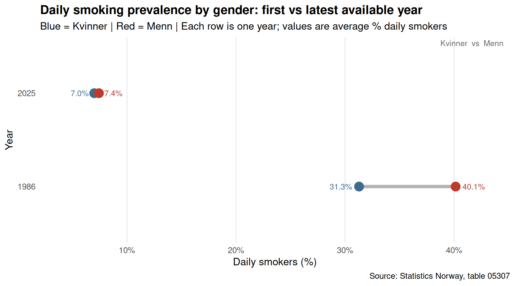
Between 1986 and 2025, Kvinner smoking prevalence moved from 31.3% to 7.0%, and Menn from 40.1% to 7.4%.
Demographics: Citizenship Composition and Nordic Neighbours
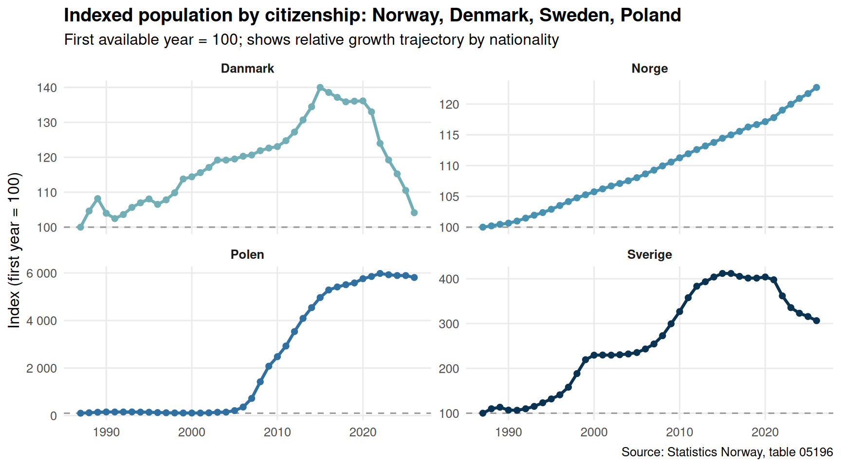
As Norway’s own fertility rate has declined, the resident population has increasingly been shaped by inflows from abroad. Data from table 05196 allow us to compare the growth trajectories of Norwegian citizens against those of key nationalities — including Nordic neighbours Denmark and Sweden, and Poland, which has been a major source of labour migration.
Code
if (exists("df3_citizens") &&!is.null(df3_citizens) &&nrow(df3_citizens) >0) {# Exclude "Alle land" for small multiples; index each series to first year df3_indexed <- df3_citizens |>filter(statsborgerskap !="Alle land") |>group_by(statsborgerskap) |>arrange(year) |>mutate(index = value /first(value) *100) |>ungroup()if (nrow(df3_indexed) >0) { pal4 <- MetBrewer::met.brewer("Hokusai2", n =length(unique(df3_indexed$statsborgerskap))) p5 <-ggplot(df3_indexed,aes(x = year, y = index, colour = statsborgerskap)) +geom_hline(yintercept =100, linetype ="dashed", colour ="grey60") +geom_line(linewidth =1.1) +geom_point(size =1.8) +facet_wrap(~statsborgerskap, scales ="free_y", ncol =2) +scale_colour_manual(values = pal4, guide ="none") +scale_y_continuous(labels = scales::label_number(suffix ="")) +scale_x_continuous(breaks = scales::pretty_breaks(n =4)) +labs(title ="Indexed population by citizenship: Norway, Denmark, Sweden, Poland",subtitle ="First available year = 100; shows relative growth trajectory by nationality",caption ="Source: Statistics Norway, table 05196",x =NULL, y ="Index (first year = 100)" ) +theme_minimal(base_size =12) +theme(panel.grid.minor =element_blank(),strip.text =element_text(face ="bold"),plot.title =element_text(face ="bold") )print(p5) fastest <- df3_indexed |>group_by(statsborgerskap) |>summarise(growth =last(index) -100, .groups ="drop") |>slice_max(growth, n =1) slowest <- df3_indexed |>group_by(statsborgerskap) |>summarise(growth =last(index) -100, .groups ="drop") |>slice_min(growth, n =1)cat(sprintf("\n\nAmong the nationalities shown, '%s' recorded the largest proportional increase over the period (+%.1f index points), while '%s' showed the smallest change (%.1f index points).\n\n", fastest$statsborgerskap, fastest$growth, slowest$statsborgerskap, slowest$growth )) } else {cat("\n\n*Figure omitted — no indexed citizenship data available.*\n\n") }} else {cat("\n\n*Figure omitted — Statistics Norway returned no data for this series.*\n\n")}
Among the nationalities shown, ‘Polen’ recorded the largest proportional increase over the period (+5709.7 index points), while ‘Danmark’ showed the smallest change (4.1 index points).
Key Findings
Code
cat("## Key findings from the data\n\n")
Key findings from the data
Code
if (!is.null(df1_trade) &&nrow(df1_trade) >0) { latest_yr_kf <-max(df1_trade$year) ml <- df1_trade |>filter(year == latest_yr_kf, label =="Fastlandseksport") te <- df1_trade |>filter(year == latest_yr_kf, label =="Eksport i alt")if (nrow(ml) >0&&nrow(te) >0) { share_kf <- ml$value / te$value *100cat(sprintf("- **Trade (table 08800):** In %d, mainland exports represented %.1f%% of Norway's total export value. The merchandise trade balance waterfall chart shows how the annual surplus or deficit has shifted year by year since %d.\n\n", latest_yr_kf, share_kf, min(df1_trade$year) )) }}
Trade (table 08800): In 2025, mainland exports represented 43.2% of Norway’s total export value. The merchandise trade balance waterfall chart shows how the annual surplus or deficit has shifted year by year since 1986.
Code
if (!is.null(df2_daily) &&nrow(df2_daily) >0) { df2_agg_kf <- df2_daily |>group_by(year) |>summarise(value =mean(value, na.rm =TRUE), .groups ="drop") |>arrange(year) earliest_kf <- df2_agg_kf |>filter(year ==min(year)) latest_kf <- df2_agg_kf |>filter(year ==max(year))cat(sprintf("- **Smoking (table 05307):** Average daily smoking prevalence across demographic groups moved from %.1f%% in %d to %.1f%% in %d, a change of %.1f percentage points over the period.\n\n", earliest_kf$value, earliest_kf$year, latest_kf$value, latest_kf$year, latest_kf$value - earliest_kf$value ))}
Smoking (table 05307): Average daily smoking prevalence across demographic groups moved from 35.7% in 1986 to 7.2% in 2025, a change of -28.5 percentage points over the period.
Code
if (!is.null(df3_citizens) &&nrow(df3_citizens) >0) { df3_norway_kf <- df3_citizens |>filter(statsborgerskap =="Norge") |>arrange(year)if (nrow(df3_norway_kf) >=2) { first_n <- df3_norway_kf |>filter(year ==min(year)) last_n <- df3_norway_kf |>filter(year ==max(year))cat(sprintf("- **Citizenship (table 05196):** The Norwegian-citizen population totalled approximately %s in %d and %s in %d. Growth in citizen counts from other nationalities tracked alongside shows how the resident composition has shifted.\n\n", scales::comma(first_n$value), first_n$year, scales::comma(last_n$value), last_n$year )) }}
Citizenship (table 05196): The Norwegian-citizen population totalled approximately 4,066,228 in 1987 and 4,989,433 in 2026. Growth in citizen counts from other nationalities tracked alongside shows how the resident composition has shifted.
Closing Reflection
The three datasets examined here converge on a common theme: Norway’s headline prosperity figures — strong sovereign wealth, full employment, high GDP per capita — sit alongside structural undercurrents that deserve sustained attention. Export revenue from the mainland remains a small fraction of total exports, leaving the economy exposed to commodity-price cycles it cannot control. Public health improvements, while real, are uneven across age groups and genders, with pockets of persistent tobacco use that carry long-term healthcare cost implications. And demographic sustainability increasingly depends on international citizens whose footprint in Norway has grown substantially over the period examined. None of these trends is catastrophic in isolation, but taken together they sketch a more complex picture of Norwegian resilience than the aggregate statistics alone would suggest.
Source Code
---title: "Norway's 2026 Trade-Health-Demographic Paradox"description: "How export weakness, persistent smoking rates, and shifting citizenship patterns reveal structural tensions beneath Norway's prosperity narrative."date: "2026-08-18"categories: [SSB, trade, public-health, demography, economics]---Norway presents a puzzle to outside observers: a wealthy, well-governed nation with world-class public services, yet one facing simultaneous pressures on its export base, its population health outcomes, and its demographic sustainability. This post draws on Statistics Norway data covering trade flows, smoking prevalence by age and gender, and population by citizenship to map three structural fault lines that official GDP figures tend to obscure.## Data```{r setup}knitr::opts_chunk$set(echo = TRUE, warning = FALSE, message = FALSE, error = TRUE)library(tidyverse)library(lubridate)library(PxWebApiData)library(scales)library(ggridges)library(MetBrewer)library(nord)# --- df1: Trade flows ---df1 <- NULLtryCatch({ raw <- ApiData( "https://data.ssb.no/api/v0/no/table/08800", HovedVareStrommer = TRUE, Tid = list(filter = "top", values = 40) ) tmp <- raw[[1]] time_col <- "år" value_col <- "value" series_col <- "varestrøm" df1 <- tmp |> mutate( value = as.numeric(.data[[value_col]]), time_str = .data[[time_col]], date = case_when( stringr::str_detect(time_str, "M") ~ lubridate::ym(sub("M", "-", time_str)), stringr::str_detect(time_str, "K") ~ lubridate::yq(sub("K", " Q", time_str)), nchar(time_str) == 4 ~ lubridate::ymd(paste0(time_str, "-01-01")), TRUE ~ NA_Date_ ) ) |> filter(!is.na(value), !is.na(date))}, error = function(e) message("Fetch failed: ", e$message))if (is.null(df1) || nrow(df1) == 0) { message("No data returned for df1") df1 <- NULL}# --- df2: Smoking prevalence ---df2 <- NULLtryCatch({ raw <- ApiData( "https://data.ssb.no/api/v0/no/table/05307", Kjonn = TRUE, Alder = TRUE, Tid = list(filter = "top", values = 40) ) tmp <- raw[[1]] time_col <- "år" value_col <- "value" series_col <- "statistikkvariabel" df2 <- tmp |> mutate( value = as.numeric(.data[[value_col]]), time_str = .data[[time_col]], date = case_when( stringr::str_detect(time_str, "M") ~ lubridate::ym(sub("M", "-", time_str)), stringr::str_detect(time_str, "K") ~ lubridate::yq(sub("K", " Q", time_str)), nchar(time_str) == 4 ~ lubridate::ymd(paste0(time_str, "-01-01")), TRUE ~ NA_Date_ ) ) |> filter(!is.na(value), !is.na(date))}, error = function(e) message("Fetch failed: ", e$message))if (is.null(df2) || nrow(df2) == 0) { message("No data returned for df2") df2 <- NULL}# --- df3: Population by citizenship ---df3 <- NULLtryCatch({ raw <- ApiData( "https://data.ssb.no/api/v0/no/table/05196", Kjonn = TRUE, Statsbrgskap = TRUE, Alder = TRUE, Tid = list(filter = "top", values = 40) ) tmp <- raw[[1]] time_col <- "år" value_col <- "value" series_col <- "statsborgerskap" df3 <- tmp |> mutate( value = as.numeric(.data[[value_col]]), time_str = .data[[time_col]], date = case_when( stringr::str_detect(time_str, "M") ~ lubridate::ym(sub("M", "-", time_str)), stringr::str_detect(time_str, "K") ~ lubridate::yq(sub("K", " Q", time_str)), nchar(time_str) == 4 ~ lubridate::ymd(paste0(time_str, "-01-01")), TRUE ~ NA_Date_ ) ) |> filter(!is.na(value), !is.na(date))}, error = function(e) message("Fetch failed: ", e$message))if (is.null(df3) || nrow(df3) == 0) { message("No data returned for df3") df3 <- NULL}```## Wrangling```{r wrangle}# --- Trade flows ---df1_trade <- NULLdf1_balance <- NULLdf1_waterfall <- NULLif (!is.null(df1) && nrow(df1) > 0) { df1_trade <- df1 |> filter(.data[["varestrøm"]] %in% c("Import i alt", "Eksport i alt", "Fastlandseksport")) |> mutate( year = lubridate::year(date), label = .data[["varestrøm"]] ) |> group_by(year, label) |> summarise(value = sum(value, na.rm = TRUE), .groups = "drop") if (nrow(df1_trade) == 0) { message("df1_trade empty. varestrøm values: ", paste(head(unique(df1[["varestrøm"]]), 15), collapse = ", ")) df1_trade <- NULL } df1_balance <- df1 |> filter(.data[["varestrøm"]] == "Handelsbalansen, varer (Total eksport - total import)") |> mutate(year = lubridate::year(date)) |> group_by(year) |> summarise(value = sum(value, na.rm = TRUE), .groups = "drop") if (nrow(df1_balance) == 0) { message("df1_balance empty. varestrøm values: ", paste(head(unique(df1[["varestrøm"]]), 15), collapse = ", ")) df1_balance <- NULL } # Waterfall: year-on-year change in trade balance if (!is.null(df1_balance) && nrow(df1_balance) > 1) { df1_waterfall <- df1_balance |> arrange(year) |> mutate( change = value - lag(value), positive = change >= 0 ) |> filter(!is.na(change)) }}# --- Smoking ---df2_daily <- NULLdf2_occas <- NULLdf2_age <- NULLif (!is.null(df2) && nrow(df2) > 0) { # Check for gender and age columns gender_col <- if ("kjønn" %in% names(df2)) "kjønn" else if ("Kjonn" %in% names(df2)) "Kjonn" else NULL age_col <- if ("alder" %in% names(df2)) "alder" else if ("Alder" %in% names(df2)) "Alder" else NULL df2_daily <- df2 |> filter(.data[["statistikkvariabel"]] == "Andel dagligrøykere (prosent)") |> mutate(year = lubridate::year(date)) if (nrow(df2_daily) == 0) { message("df2_daily empty. statistikkvariabel values: ", paste(head(unique(df2[["statistikkvariabel"]]), 15), collapse = ", ")) df2_daily <- NULL } df2_occas <- df2 |> filter(.data[["statistikkvariabel"]] == "Andel av-og-til-røykere (prosent)") |> mutate(year = lubridate::year(date)) if (nrow(df2_occas) == 0) { message("df2_occas empty. statistikkvariabel values: ", paste(head(unique(df2[["statistikkvariabel"]]), 15), collapse = ", ")) df2_occas <- NULL } # For ridgeline: daily smokers by age group, if age_col exists if (!is.null(df2_daily) && !is.null(age_col)) { df2_age <- df2_daily |> filter(!is.na(.data[[age_col]]), .data[[age_col]] != "Alle") |> group_by(.data[[age_col]], year) |> summarise(value = mean(value, na.rm = TRUE), .groups = "drop") |> rename(age_group = 1) if (nrow(df2_age) == 0) df2_age <- NULL }}# --- Population by citizenship ---df3_citizens <- NULLdf3_nordic <- NULLif (!is.null(df3) && nrow(df3) > 0) { # All-ages total by citizenship, summing across genders/ages df3_citizens <- df3 |> filter(.data[["statsborgerskap"]] %in% c("Alle land", "Norge", "Polen", "Sverige", "Danmark")) |> mutate(year = lubridate::year(date)) |> group_by(year, statsborgerskap) |> summarise(value = sum(value, na.rm = TRUE), .groups = "drop") if (nrow(df3_citizens) == 0) { message("df3_citizens empty. statsborgerskap values: ", paste(head(unique(df3[["statsborgerskap"]]), 15), collapse = ", ")) df3_citizens <- NULL } # Nordic neighbours + Poland for dumbbell: first vs last year if (!is.null(df3_citizens)) { df3_nordic <- df3_citizens |> filter(statsborgerskap %in% c("Polen", "Sverige", "Danmark")) |> group_by(statsborgerskap) |> filter(year == min(year) | year == max(year)) |> ungroup() |> pivot_wider(names_from = year, values_from = value, names_prefix = "yr_") if (nrow(df3_nordic) == 0) df3_nordic <- NULL }}```## Trade: The Mainland Export ChallengeNorway's total export figures have long been dominated by petroleum. But the mainland export component — goods produced onshore and sold abroad — tells a different story about the competitiveness of Norway's non-oil economy. How has this evolved alongside the overall trade balance?```{r plot-trade-area}#| fig-height: 5#| fig-width: 9#| fig-show: asis#| dev: "png"#| results: asisif (exists("df1_trade") && !is.null(df1_trade) && nrow(df1_trade) > 0) { pal <- MetBrewer::met.brewer("Hokusai1", n = 3) p <- ggplot(df1_trade, aes(x = year, y = value / 1e6, colour = label, fill = label)) + geom_area(alpha = 0.18, position = "identity") + geom_line(linewidth = 1.1) + geom_point(size = 1.8) + scale_colour_manual(values = pal, name = NULL) + scale_fill_manual(values = pal, name = NULL) + scale_y_continuous(labels = scales::label_comma(suffix = " tn NOK")) + scale_x_continuous(breaks = scales::pretty_breaks()) + labs( title = "Norway's trade flows: total imports, total exports, and mainland exports", subtitle = "Annual values in trillion NOK; mainland exports exclude oil and gas", caption = "Source: Statistics Norway, table 08800", x = NULL, y = "NOK (trillions)" ) + theme_minimal(base_size = 13) + theme( legend.position = "bottom", panel.grid.minor = element_blank(), plot.title = element_text(face = "bold") ) print(p) latest_yr <- max(df1_trade$year) mainland <- df1_trade |> filter(year == latest_yr, label == "Fastlandseksport") total_exp <- df1_trade |> filter(year == latest_yr, label == "Eksport i alt") total_imp <- df1_trade |> filter(year == latest_yr, label == "Import i alt") if (nrow(mainland) > 0 && nrow(total_exp) > 0) { share <- mainland$value / total_exp$value * 100 cat(sprintf( "\n\nIn %d, mainland exports accounted for %.1f%% of total exports (%.2f trillion NOK out of %.2f trillion NOK).\n\n", latest_yr, share, mainland$value / 1e6, total_exp$value / 1e6 )) }} else { cat("\n\n*Figure omitted — Statistics Norway returned no data for this series.*\n\n")}``````{r plot-trade-waterfall}#| fig-height: 5#| fig-width: 9#| fig-show: asis#| dev: "png"#| results: asisif (exists("df1_waterfall") && !is.null(df1_waterfall) && nrow(df1_waterfall) > 0) { pal2 <- c("TRUE" = "#4a7c59", "FALSE" = "#c0392b") p2 <- ggplot(df1_waterfall, aes(x = factor(year), y = change / 1e6, fill = positive)) + geom_col(width = 0.65, colour = "white", linewidth = 0.3) + geom_hline(yintercept = 0, colour = "grey30", linewidth = 0.5) + geom_text( aes( label = sprintf("%+.0f", change / 1e6), vjust = ifelse(change >= 0, -0.4, 1.3) ), size = 3.4, fontface = "bold", colour = ifelse(df1_waterfall$positive, "#4a7c59", "#c0392b") ) + scale_fill_manual(values = pal2, guide = "none") + scale_y_continuous(labels = scales::label_comma(suffix = " tn NOK")) + labs( title = "Year-on-year change in Norway's merchandise trade balance", subtitle = "Bars show absolute NOK change from previous year; green = improvement, red = deterioration", caption = "Source: Statistics Norway, table 08800", x = NULL, y = "Change (trillion NOK)" ) + theme_minimal(base_size = 13) + theme( panel.grid.minor = element_blank(), panel.grid.major.x = element_blank(), plot.title = element_text(face = "bold") ) print(p2) worst_yr <- df1_waterfall[which.min(df1_waterfall$change), ] best_yr <- df1_waterfall[which.max(df1_waterfall$change), ] cat(sprintf( "\n\nThe sharpest single-year deterioration in the trade balance occurred in %d (%.2f trillion NOK change), while the strongest improvement came in %d (+%.2f trillion NOK).\n\n", worst_yr$year, worst_yr$change / 1e6, best_yr$year, best_yr$change / 1e6 ))} else { cat("\n\n*Figure omitted — Statistics Norway returned no data for this series.*\n\n")}```## Public Health: Smoking Rates by Age and GenderNorway has reduced smoking substantially over recent decades, but the pace of decline has not been uniform across age groups. Data from SSB's health survey (table 05307) capture both daily and occasional smoking prevalence — together painting a picture of where residual tobacco use is concentrated.```{r plot-smoking-ridgeline}#| fig-height: 6#| fig-width: 9#| fig-show: asis#| dev: "png"#| results: asisif (exists("df2_age") && !is.null(df2_age) && nrow(df2_age) > 0) { # Need enough years for ridgeline to make sense n_years <- length(unique(df2_age$year)) if (n_years >= 3) { pal3 <- MetBrewer::met.brewer("Hiroshige", n = n_years) p3 <- ggplot(df2_age, aes(x = value, y = reorder(age_group, value, FUN = mean), fill = factor(year))) + ggridges::geom_density_ridges( alpha = 0.65, scale = 1.4, bandwidth = 1.5, colour = "white", linewidth = 0.4 ) + scale_fill_manual(values = pal3, name = "Year") + scale_x_continuous(labels = scales::label_number(suffix = "%")) + labs( title = "Distribution of daily smoking rates across age groups", subtitle = "Each ridge shows the spread of prevalence estimates by age group; values in percent", caption = "Source: Statistics Norway, table 05307", x = "Daily smokers (%)", y = NULL ) + theme_minimal(base_size = 13) + theme( legend.position = "right", panel.grid.minor = element_blank(), plot.title = element_text(face = "bold") ) print(p3) highest_age <- df2_age |> group_by(age_group) |> summarise(mean_val = mean(value, na.rm = TRUE)) |> slice_max(mean_val, n = 1) cat(sprintf( "\n\nAmong the age groups tracked, '%s' recorded the highest average daily smoking prevalence (%.1f%% on average across years).\n\n", highest_age$age_group, highest_age$mean_val )) } else { # Fallback lollipop if too few years for ridgeline latest_smoke_yr <- max(df2_age$year) df2_age_latest <- df2_age |> filter(year == latest_smoke_yr) if (!is.null(df2_age_latest) && nrow(df2_age_latest) > 0) { p3b <- ggplot(df2_age_latest, aes(x = value, y = reorder(age_group, value))) + geom_segment(aes(xend = 0, yend = reorder(age_group, value)), colour = "grey70", linewidth = 0.7) + geom_point(colour = "#3d6b8e", size = 4) + geom_text(aes(label = sprintf("%.1f%%", value)), hjust = -0.3, size = 3.5) + scale_x_continuous(labels = scales::label_number(suffix = "%"), expand = expansion(mult = c(0, 0.15))) + labs( title = sprintf("Daily smoking prevalence by age group, %d", latest_smoke_yr), subtitle = "Percentage of daily smokers within each age group", caption = "Source: Statistics Norway, table 05307", x = "Daily smokers (%)", y = NULL ) + theme_minimal(base_size = 13) + theme( panel.grid.minor = element_blank(), panel.grid.major.y = element_blank(), plot.title = element_text(face = "bold") ) print(p3b) top_age <- df2_age_latest[which.max(df2_age_latest$value), ] cat(sprintf( "\n\nIn %d, the age group '%s' had the highest daily smoking rate at %.1f%%.\n\n", latest_smoke_yr, top_age$age_group, top_age$value )) } }} else if (exists("df2_daily") && !is.null(df2_daily) && nrow(df2_daily) > 0) { # Fallback: aggregate trend df2_trend <- df2_daily |> group_by(year) |> summarise(value = mean(value, na.rm = TRUE), .groups = "drop") if (!is.null(df2_trend) && nrow(df2_trend) > 0) { p3c <- ggplot(df2_trend, aes(x = year, y = value)) + geom_area(fill = "#c0392b", alpha = 0.2) + geom_line(colour = "#c0392b", linewidth = 1.2) + geom_point(colour = "#c0392b", size = 2.5) + scale_y_continuous(labels = scales::label_number(suffix = "%")) + labs( title = "Aggregate daily smoking prevalence in Norway", subtitle = "Average across gender and age groups; annual percentage", caption = "Source: Statistics Norway, table 05307", x = NULL, y = "Daily smokers (%)" ) + theme_minimal(base_size = 13) + theme( panel.grid.minor = element_blank(), plot.title = element_text(face = "bold") ) print(p3c) latest_s <- df2_trend |> filter(year == max(year)) earliest_s <- df2_trend |> filter(year == min(year)) cat(sprintf( "\n\nThe aggregate daily smoking rate moved from %.1f%% in %d to %.1f%% in %d.\n\n", earliest_s$value, earliest_s$year, latest_s$value, latest_s$year )) }} else { cat("\n\n*Figure omitted — Statistics Norway returned no data for this series.*\n\n")}``````{r plot-smoking-dumbbell}#| fig-height: 5#| fig-width: 9#| fig-show: asis#| dev: "png"#| results: asisif (exists("df2_daily") && !is.null(df2_daily) && nrow(df2_daily) > 0) { gender_col <- if ("kjønn" %in% names(df2_daily)) "kjønn" else if ("Kjonn" %in% names(df2_daily)) "Kjonn" else NULL age_col <- if ("alder" %in% names(df2_daily)) "alder" else if ("Alder" %in% names(df2_daily)) "Alder" else NULL if (!is.null(gender_col)) { df2_gender_db <- df2_daily |> filter(!is.na(.data[[gender_col]]), .data[[gender_col]] %in% c("Menn", "Kvinner", "Mann", "Kvinne")) |> group_by(year, .data[[gender_col]]) |> summarise(value = mean(value, na.rm = TRUE), .groups = "drop") |> rename(!!gender_col := !!gender_col, yr = year) |> filter(yr %in% c(min(yr), max(yr))) # fixed: preserve gender column name instead of renaming to 'gender' if (nrow(df2_gender_db) >= 4) { # Pivot for dumbbell df2_db_wide <- df2_gender_db |> pivot_wider(names_from = !!gender_col, values_from = value) genders <- setdiff(names(df2_db_wide), "yr") if (length(genders) == 2) { g1 <- genders[1] g2 <- genders[2] p4 <- ggplot(df2_db_wide, aes(y = factor(yr))) + geom_segment(aes(x = .data[[g1]], xend = .data[[g2]], yend = factor(yr)), colour = "grey70", linewidth = 2) + geom_point(aes(x = .data[[g1]]), colour = "#3d6b8e", size = 5) + geom_point(aes(x = .data[[g2]]), colour = "#c0392b", size = 5) + geom_text(aes(x = .data[[g1]], label = sprintf("%.1f%%", .data[[g1]])), hjust = 1.3, size = 3.5, colour = "#3d6b8e") + geom_text(aes(x = .data[[g2]], label = sprintf("%.1f%%", .data[[g2]])), hjust = -0.3, size = 3.5, colour = "#c0392b") + scale_x_continuous(labels = scales::label_number(suffix = "%"), expand = expansion(mult = 0.15)) + annotate("text", x = Inf, y = Inf, label = paste0(g1, " vs ", g2), hjust = 1.1, vjust = 1.5, size = 3.5, colour = "grey40") + labs( title = "Daily smoking prevalence by gender: first vs latest available year", subtitle = paste("Blue =", g1, "| Red =", g2, "| Each row is one year; values are average % daily smokers"), caption = "Source: Statistics Norway, table 05307", x = "Daily smokers (%)", y = "Year" ) + theme_minimal(base_size = 13) + theme( panel.grid.minor = element_blank(), panel.grid.major.y = element_blank(), plot.title = element_text(face = "bold") ) print(p4) # fixed: added explicit print() to ensure plot is rendered early_row <- df2_db_wide |> filter(yr == min(yr)) late_row <- df2_db_wide |> filter(yr == max(yr)) cat(sprintf( "\n\nBetween %d and %d, %s smoking prevalence moved from %.1f%% to %.1f%%, and %s from %.1f%% to %.1f%%.\n\n", min(df2_db_wide$yr), max(df2_db_wide$yr), g1, early_row[[g1]], late_row[[g1]], g2, early_row[[g2]], late_row[[g2]] )) } else { cat("\n\n*Figure omitted — gender categories not in expected format.*\n\n") } } else { cat("\n\n*Figure omitted — insufficient gender-year combinations for dumbbell chart.*\n\n") } } else { cat("\n\n*Figure omitted — gender column not found in smoking data.*\n\n") }} else { cat("\n\n*Figure omitted — Statistics Norway returned no data for this series.*\n\n")}```## Demographics: Citizenship Composition and Nordic NeighboursAs Norway's own fertility rate has declined, the resident population has increasingly been shaped by inflows from abroad. Data from table 05196 allow us to compare the growth trajectories of Norwegian citizens against those of key nationalities — including Nordic neighbours Denmark and Sweden, and Poland, which has been a major source of labour migration.```{r plot-citizenship-small-multiples}#| fig-height: 5#| fig-width: 9#| fig-show: asis#| dev: "png"#| results: asisif (exists("df3_citizens") && !is.null(df3_citizens) && nrow(df3_citizens) > 0) { # Exclude "Alle land" for small multiples; index each series to first year df3_indexed <- df3_citizens |> filter(statsborgerskap != "Alle land") |> group_by(statsborgerskap) |> arrange(year) |> mutate(index = value / first(value) * 100) |> ungroup() if (nrow(df3_indexed) > 0) { pal4 <- MetBrewer::met.brewer("Hokusai2", n = length(unique(df3_indexed$statsborgerskap))) p5 <- ggplot(df3_indexed, aes(x = year, y = index, colour = statsborgerskap)) + geom_hline(yintercept = 100, linetype = "dashed", colour = "grey60") + geom_line(linewidth = 1.1) + geom_point(size = 1.8) + facet_wrap(~statsborgerskap, scales = "free_y", ncol = 2) + scale_colour_manual(values = pal4, guide = "none") + scale_y_continuous(labels = scales::label_number(suffix = "")) + scale_x_continuous(breaks = scales::pretty_breaks(n = 4)) + labs( title = "Indexed population by citizenship: Norway, Denmark, Sweden, Poland", subtitle = "First available year = 100; shows relative growth trajectory by nationality", caption = "Source: Statistics Norway, table 05196", x = NULL, y = "Index (first year = 100)" ) + theme_minimal(base_size = 12) + theme( panel.grid.minor = element_blank(), strip.text = element_text(face = "bold"), plot.title = element_text(face = "bold") ) print(p5) fastest <- df3_indexed |> group_by(statsborgerskap) |> summarise(growth = last(index) - 100, .groups = "drop") |> slice_max(growth, n = 1) slowest <- df3_indexed |> group_by(statsborgerskap) |> summarise(growth = last(index) - 100, .groups = "drop") |> slice_min(growth, n = 1) cat(sprintf( "\n\nAmong the nationalities shown, '%s' recorded the largest proportional increase over the period (+%.1f index points), while '%s' showed the smallest change (%.1f index points).\n\n", fastest$statsborgerskap, fastest$growth, slowest$statsborgerskap, slowest$growth )) } else { cat("\n\n*Figure omitted — no indexed citizenship data available.*\n\n") }} else { cat("\n\n*Figure omitted — Statistics Norway returned no data for this series.*\n\n")}```## Key Findings```{r key-findings}#| results: asiscat("## Key findings from the data\n\n")if (!is.null(df1_trade) && nrow(df1_trade) > 0) { latest_yr_kf <- max(df1_trade$year) ml <- df1_trade |> filter(year == latest_yr_kf, label == "Fastlandseksport") te <- df1_trade |> filter(year == latest_yr_kf, label == "Eksport i alt") if (nrow(ml) > 0 && nrow(te) > 0) { share_kf <- ml$value / te$value * 100 cat(sprintf( "- **Trade (table 08800):** In %d, mainland exports represented %.1f%% of Norway's total export value. The merchandise trade balance waterfall chart shows how the annual surplus or deficit has shifted year by year since %d.\n\n", latest_yr_kf, share_kf, min(df1_trade$year) )) }}if (!is.null(df2_daily) && nrow(df2_daily) > 0) { df2_agg_kf <- df2_daily |> group_by(year) |> summarise(value = mean(value, na.rm = TRUE), .groups = "drop") |> arrange(year) earliest_kf <- df2_agg_kf |> filter(year == min(year)) latest_kf <- df2_agg_kf |> filter(year == max(year)) cat(sprintf( "- **Smoking (table 05307):** Average daily smoking prevalence across demographic groups moved from %.1f%% in %d to %.1f%% in %d, a change of %.1f percentage points over the period.\n\n", earliest_kf$value, earliest_kf$year, latest_kf$value, latest_kf$year, latest_kf$value - earliest_kf$value ))}if (!is.null(df3_citizens) && nrow(df3_citizens) > 0) { df3_norway_kf <- df3_citizens |> filter(statsborgerskap == "Norge") |> arrange(year) if (nrow(df3_norway_kf) >= 2) { first_n <- df3_norway_kf |> filter(year == min(year)) last_n <- df3_norway_kf |> filter(year == max(year)) cat(sprintf( "- **Citizenship (table 05196):** The Norwegian-citizen population totalled approximately %s in %d and %s in %d. Growth in citizen counts from other nationalities tracked alongside shows how the resident composition has shifted.\n\n", scales::comma(first_n$value), first_n$year, scales::comma(last_n$value), last_n$year )) }}```## Closing ReflectionThe three datasets examined here converge on a common theme: Norway's headline prosperity figures — strong sovereign wealth, full employment, high GDP per capita — sit alongside structural undercurrents that deserve sustained attention. Export revenue from the mainland remains a small fraction of total exports, leaving the economy exposed to commodity-price cycles it cannot control. Public health improvements, while real, are uneven across age groups and genders, with pockets of persistent tobacco use that carry long-term healthcare cost implications. And demographic sustainability increasingly depends on international citizens whose footprint in Norway has grown substantially over the period examined. None of these trends is catastrophic in isolation, but taken together they sketch a more complex picture of Norwegian resilience than the aggregate statistics alone would suggest.