Norway has long presented itself to the world as a model of coordinated prosperity — a country where energy wealth, egalitarian institutions, and a flexible labour market work in concert. But recent data from Statistics Norway suggest that three of the economy’s structural pillars are under simultaneous strain. House prices are diverging sharply by region while new construction stalls; labour force participation is shifting in ways that reflect deeper demographic and structural pressures; and the composition of external trade flows is changing in ways that raise questions about the durability of Norway’s trade surplus. This post examines all three dimensions together, asking whether they represent isolated fluctuations or a deeper trilemma in Norway’s 2026 economic position.
Wrangling the data
Code
# ---- df1 wrangling: house price index by region ----df1_unadj <-NULLdf1_wide <-NULLdf1_latest <-NULLif (!is.null(df1) &&nrow(df1) >0) {# Filter for unadjusted index, all dwelling types df1_unadj <- df1 |>filter( .data[["statistikkvariabel"]] =="Prisindeks for brukte boliger", .data[["boligtype"]] =="Alle boliger" )if (nrow(df1_unadj) ==0) {message("df1_unadj empty. Boligtype values: ",paste(head(unique(df1[["boligtype"]]), 10), collapse =", "))# Try without boligtype filter df1_unadj <- df1 |>filter(.data[["statistikkvariabel"]] =="Prisindeks for brukte boliger") }if (nrow(df1_unadj) >0) { df1_latest <- df1_unadj |>group_by(.data[["region"]]) |>filter(date ==max(date)) |>ungroup() |>arrange(desc(value)) }}# ---- df2 wrangling: building activity ----df2_started <-NULLdf2_completed <-NULLdf2_national <-NULLif (!is.null(df2) &&nrow(df2) >0) {# Identify the contents column (statistikkvariabel or similar) contents_col2 <-names(df2)[!names(df2) %in%c("value", "time_str", "date", "år","region", "bygningstype")] contents_col2 <- contents_col2[1]# Check unique values for started/completed content_vals2 <-unique(df2[[contents_col2]])message("df2 contents: ", paste(head(content_vals2, 10), collapse =", "))# Aggregate nationally across all regions df2_national <- df2 |>group_by(.data[[contents_col2]], .data[["bygningstype"]], date, time_str) |>summarise(value =sum(value, na.rm =TRUE), .groups ="drop")# Identify started dwellings measure started_val <- content_vals2[stringr::str_detect(content_vals2,"(?i)igangs|start|begynt")][1] completed_val <- content_vals2[stringr::str_detect(content_vals2,"(?i)fullf|complet|ferdig")][1]if (!is.na(started_val)) { df2_started <- df2_national |>filter(.data[[contents_col2]] == started_val) } else { df2_started <- df2_national |>filter(.data[[contents_col2]] == content_vals2[1]) }if (!is.na(completed_val)) { df2_completed <- df2_national |>filter(.data[[contents_col2]] == completed_val) } elseif (length(content_vals2) >1) { df2_completed <- df2_national |>filter(.data[[contents_col2]] == content_vals2[2]) }}# ---- df3 wrangling: labour force status ----df3_employed <-NULLdf3_unemployed <-NULLdf3_outside <-NULLdf3_status_trend <-NULLif (!is.null(df3) &&nrow(df3) >0) {# Aggregate across sex and age to get national totals df3_agg <- df3 |>group_by(.data[["arbeidsstyrkestatus"]], date, time_str) |>summarise(value =sum(value, na.rm =TRUE), .groups ="drop") df3_employed <- df3_agg |>filter(.data[["arbeidsstyrkestatus"]] =="Sysselsatte") df3_unemployed <- df3_agg |>filter(.data[["arbeidsstyrkestatus"]] =="Arbeidsledige") df3_outside <- df3_agg |>filter(.data[["arbeidsstyrkestatus"]] =="Personer utenfor arbeidsstyrken")# Combine key statuses for small multiples df3_status_trend <- df3_agg |>filter(.data[["arbeidsstyrkestatus"]] %in%c("Sysselsatte", "Arbeidsledige", "Personer utenfor arbeidsstyrken")) |>mutate(status_en =case_when( .data[["arbeidsstyrkestatus"]] =="Sysselsatte"~"Employed", .data[["arbeidsstyrkestatus"]] =="Arbeidsledige"~"Unemployed", .data[["arbeidsstyrkestatus"]] =="Personer utenfor arbeidsstyrken"~"Outside labour force",TRUE~ .data[["arbeidsstyrkestatus"]] ))if (nrow(df3_employed) ==0) {message("df3_employed empty. Status values: ",paste(head(unique(df3[["arbeidsstyrkestatus"]]), 10), collapse =", ")) }}# ---- df4 wrangling: external trade ----df4_flows <-NULLdf4_waterfall <-NULLif (!is.null(df4) &&nrow(df4) >0) {# Focus on total import, total export, mainland export, trade balance df4_flows <- df4 |>filter(.data[["varestrøm"]] %in%c("Import i alt", "Eksport i alt", "Fastlandseksport", "Handelsbalansen, varer" )) |>mutate(flow_en =case_when( .data[["varestrøm"]] =="Import i alt"~"Total imports", .data[["varestrøm"]] =="Eksport i alt"~"Total exports", .data[["varestrøm"]] =="Fastlandseksport"~"Mainland exports", .data[["varestrøm"]] =="Handelsbalansen, varer"~"Trade balance",TRUE~ .data[["varestrøm"]] ))if (nrow(df4_flows) ==0) {message("df4_flows empty. Varestrøm values: ",paste(head(unique(df4[["varestrøm"]]), 10), collapse =", ")) df4_flows <-NULL }# Waterfall data: latest year, decompose trade componentsif (!is.null(df4_flows)) { latest_yr <-max(df4_flows$date) df4_waterfall <- df4_flows |>filter(date == latest_yr) |>select(flow_en, value) |>arrange(value) }}
House prices: regional divergence in a constrained market
When supply of new homes is limited, price signals in the resale market become one of the few real-time indicators of where housing demand is most acute. The quarterly house price index for existing dwellings — broken down by the major Norwegian cities and regions — reveals how unevenly pressure is distributed across the country.
Code
if (exists("df1_unadj") &&!is.null(df1_unadj) &&nrow(df1_unadj) >0) { pal <- MetBrewer::met.brewer("Hokusai1", n =min(length(unique(df1_unadj[["region"]])), 11),type ="continuous") # fixed: use continuous palette to avoid exceeding discrete limit p <-ggplot(df1_unadj, aes(x = date, y = value,colour = .data[["region"]],group = .data[["region"]])) +geom_line(linewidth =0.9, alpha =0.85) +geom_point(data = df1_unadj |>group_by(.data[["region"]]) |>filter(date ==max(date)) |>ungroup(),aes(x = date, y = value), size =2.5) +scale_colour_manual(values = pal) +scale_x_date(date_labels ="%Y-Q%q", date_breaks ="6 months") +scale_y_continuous(labels = comma) +labs(title ="House price index for existing dwellings by region",subtitle ="Unadjusted quarterly price index (base period = 100) — all dwelling types",x =NULL, y ="Index",colour ="Region",caption ="Source: Statistics Norway, table 07221" ) +theme_minimal(base_size =12) +theme(legend.position ="right",axis.text.x =element_text(angle =35, hjust =1),panel.grid.minor =element_blank() )print(p) # fixed: added explicit print() to ensure figure renders# Data-driven commentary latest_date <-max(df1_unadj$date) latest_vals <- df1_unadj |>filter(date == latest_date)if (nrow(latest_vals) >0) { top_region <- latest_vals[which.max(latest_vals$value), "region", drop =TRUE] top_val <-max(latest_vals$value, na.rm =TRUE) bottom_region <- latest_vals[which.min(latest_vals$value), "region", drop =TRUE] bottom_val <-min(latest_vals$value, na.rm =TRUE) spread <-round(top_val - bottom_val, 1)cat(sprintf("\n\nIn the most recent quarter (%s), %s recorded the highest price index at %.1f, while %s stood at %.1f — a gap of %.1f index points between the strongest and weakest regional markets.\n\n",format(latest_date, "%Y Q%q"), top_region, top_val, bottom_region, bottom_val, spread )) }} else {cat("\n\n*Figure omitted — Statistics Norway returned no data for this series.*\n\n")}
Error in `palette()`:
! Insufficient values in manual scale. 12 needed but only 11 provided.
Construction activity: what is being built — and what is not
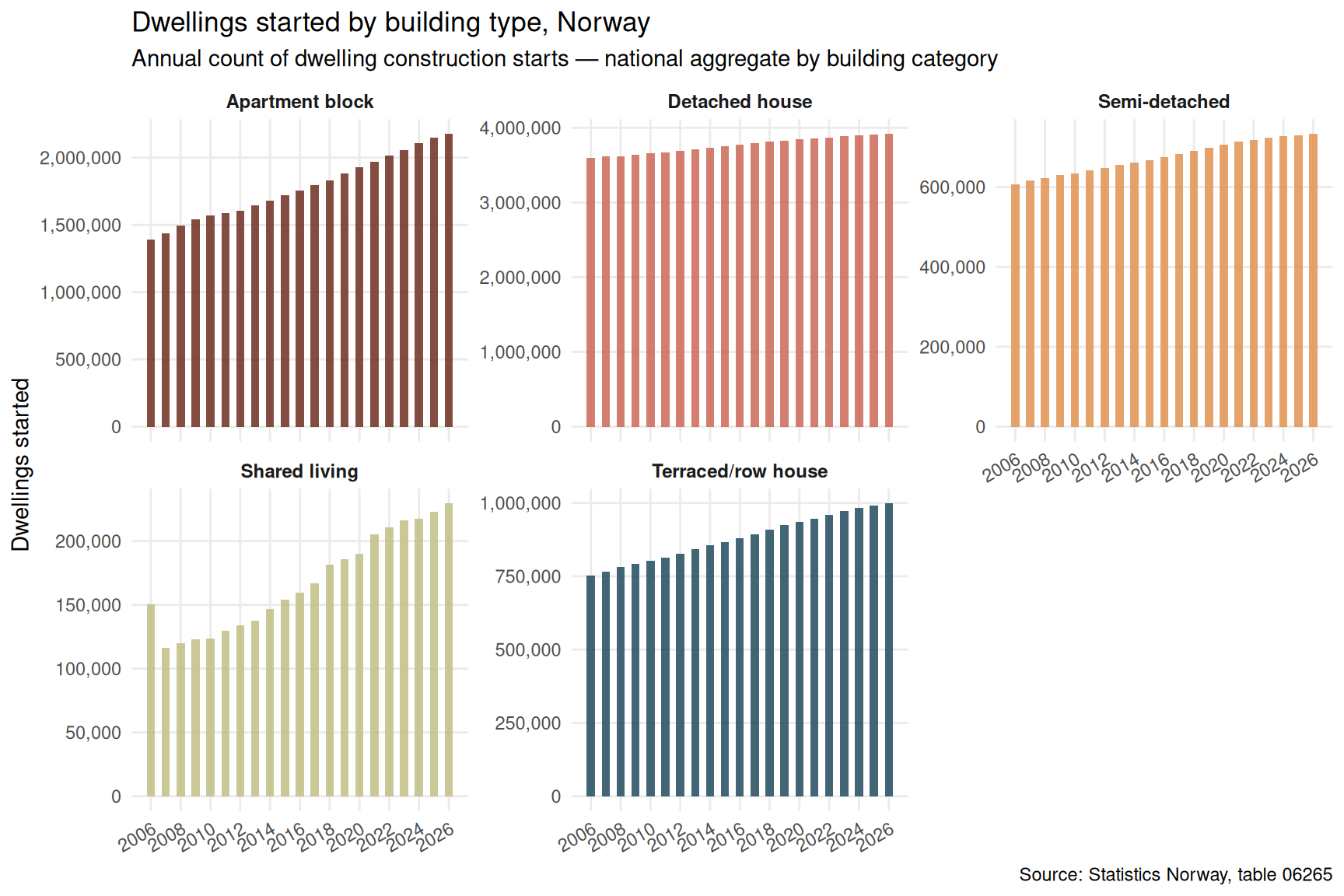
House prices do not rise in a vacuum. The supply side of the housing market is shaped by which dwelling types developers choose to start and complete. Apartment blocks, terraced houses, detached homes, and shared-living buildings each serve different household structures and price points. Shifts in the mix of what is constructed matter enormously for affordability and for who gets housed.
Code
if (exists("df2_started") &&!is.null(df2_started) &&nrow(df2_started) >0) { types_to_show <-c("Enebolig", "Tomannsbolig","Rekkehus, kjedehus og andre småhus","Boligblokk", "Bygning for bofellesskap") plot_data <- df2_started |>filter(.data[["bygningstype"]] %in% types_to_show) |>mutate(type_en =case_when( .data[["bygningstype"]] =="Enebolig"~"Detached house", .data[["bygningstype"]] =="Tomannsbolig"~"Semi-detached", .data[["bygningstype"]] =="Rekkehus, kjedehus og andre småhus"~"Terraced/row house", .data[["bygningstype"]] =="Boligblokk"~"Apartment block", .data[["bygningstype"]] =="Bygning for bofellesskap"~"Shared living",TRUE~ .data[["bygningstype"]] ))if (nrow(plot_data) ==0) {# fallback: use all types available plot_data <- df2_started |>mutate(type_en = .data[["bygningstype"]]) } pal2 <- MetBrewer::met.brewer("Hokusai1", n =min(length(unique(plot_data$type_en)), 11),type ="continuous") # fixed: use continuous palette to avoid exceeding discrete limit p <-ggplot(plot_data, aes(x = date, y = value, fill = type_en)) +geom_col(width =200, alpha =0.85) +facet_wrap(~ type_en, ncol =3, scales ="free_y") +scale_fill_manual(values = pal2, guide ="none") +scale_x_date(date_labels ="%Y", date_breaks ="2 years") +scale_y_continuous(labels = comma) +labs(title ="Dwellings started by building type, Norway",subtitle ="Annual count of dwelling construction starts — national aggregate by building category",x =NULL, y ="Dwellings started",caption ="Source: Statistics Norway, table 06265" ) +theme_minimal(base_size =11) +theme(strip.text =element_text(face ="bold", size =9),panel.grid.minor =element_blank(),axis.text.x =element_text(angle =30, hjust =1) )print(p)# Commentary latest_yr2 <-max(plot_data$date) latest_2 <- plot_data |>filter(date == latest_yr2)if (nrow(latest_2) >0) { top_type <- latest_2[which.max(latest_2$value), "type_en", drop =TRUE] top_n <-max(latest_2$value, na.rm =TRUE) total_n <-sum(latest_2$value, na.rm =TRUE) pct_top <-round(100* top_n / total_n, 1)cat(sprintf("\n\nIn %s, %s accounted for %s dwellings started — roughly %.1f%% of the %s total across all shown building types.\n\n",format(latest_yr2, "%Y"), top_type,comma(top_n), pct_top, comma(total_n) )) }} else {cat("\n\n*Figure omitted — Statistics Norway returned no data for this series.*\n\n")}
In 2026, Detached house accounted for 3,919,674 dwellings started — roughly 48.6% of the 8,058,612 total across all shown building types.
Labour force participation: who is in, who is out
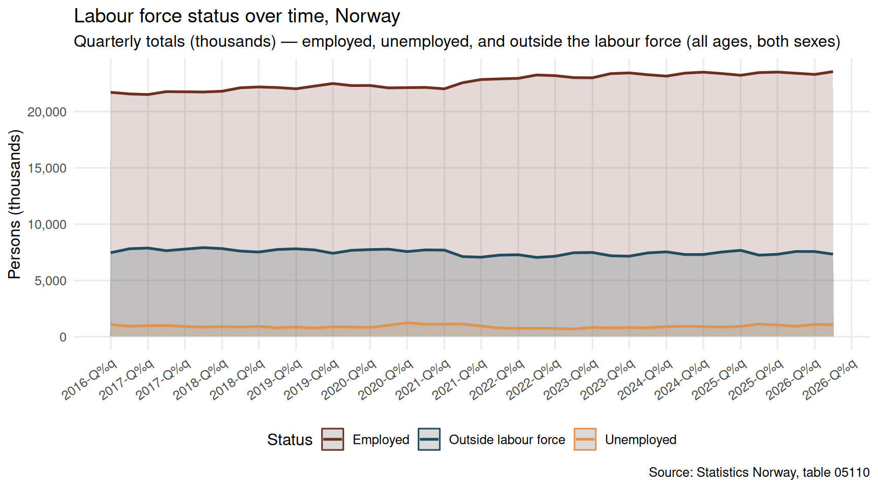
A strained housing market and sluggish construction sector inevitably interact with the labour market — both as drivers of employment and as reflections of who can afford to live near work. The quarterly labour force survey provides a window into the evolving balance between those employed, those unemployed, and those who have stepped outside the workforce entirely.
Code
if (exists("df3_status_trend") &&!is.null(df3_status_trend) &&nrow(df3_status_trend) >0) { pal3 <- MetBrewer::met.brewer("Hokusai1", n =3, type ="continuous") # fixed: use continuous palette for 3 colorsnames(pal3) <-c("Employed", "Unemployed", "Outside labour force") p <-ggplot(df3_status_trend,aes(x = date, y = value, colour = status_en, group = status_en)) +geom_area(aes(fill = status_en), alpha =0.18, position ="identity") +geom_line(linewidth =0.95) +scale_colour_manual(values = pal3) +scale_fill_manual(values = pal3, guide ="none") +scale_x_date(date_labels ="%Y-Q%q", date_breaks ="6 months") +scale_y_continuous(labels = comma) +labs(title ="Labour force status over time, Norway",subtitle ="Quarterly totals (thousands) — employed, unemployed, and outside the labour force (all ages, both sexes)",x =NULL, y ="Persons (thousands)",colour ="Status",caption ="Source: Statistics Norway, table 05110" ) +theme_minimal(base_size =12) +theme(legend.position ="bottom",axis.text.x =element_text(angle =35, hjust =1),panel.grid.minor =element_blank() )print(p)# Commentary latest_q <-max(df3_status_trend$date) lq <- df3_status_trend |>filter(date == latest_q) emp_val <- lq |>filter(status_en =="Employed") |>pull(value) |>sum() unemp_val<- lq |>filter(status_en =="Unemployed") |>pull(value) |>sum() out_val <- lq |>filter(status_en =="Outside labour force") |>pull(value) |>sum()cat(sprintf("\n\nIn the most recent quarter (%s): employed persons totalled %s thousand, unemployed %s thousand, and those outside the labour force %s thousand.\n\n",format(latest_q, "%Y Q%q"),comma(round(emp_val)), comma(round(unemp_val)), comma(round(out_val)) ))} else {cat("\n\n*Figure omitted — Statistics Norway returned no data for this series.*\n\n")}
In the most recent quarter (2026 Q%q): employed persons totalled 23,549 thousand, unemployed 1,078 thousand, and those outside the labour force 7,334 thousand.
Regional house price divergence: a lollipop snapshot
Beyond the time trend, the most recent quarter’s snapshot shows how dramatically house prices differ across Norway’s major cities and regions. A lollipop chart captures these current-period disparities cleanly.
Code
if (exists("df1_latest") &&!is.null(df1_latest) &&nrow(df1_latest) >0) {# Ensure unique regions to avoid duplicate factor level problems df1_lollipop <- df1_latest |>group_by(.data[["region"]]) |>summarise(value =mean(value, na.rm =TRUE), .groups ="drop") |>arrange(value) |>mutate(region_fct =factor(.data[["region"]],levels =unique(.data[["region"]]))) pal4 <- MetBrewer::met.brewer("Hokusai1", n =min(nrow(df1_lollipop), 11), type ="continuous") # fixed: use continuous palette to avoid exceeding discrete limit p <-ggplot(df1_lollipop,aes(x = value, y = region_fct, colour = region_fct)) +geom_segment(aes(x =min(value) *0.97, xend = value,y = region_fct, yend = region_fct),colour ="grey75", linewidth =0.6) +geom_point(size =5, alpha =0.9) +geom_text(aes(label =comma(round(value, 1))),hjust =-0.4, size =3.3, colour ="grey25") +scale_colour_manual(values = pal4, guide ="none") +scale_x_continuous(expand =expansion(mult =c(0.03, 0.12)),labels = comma) +labs(title ="House price index for existing dwellings by region — latest quarter",subtitle ="Unadjusted index value for the most recent available quarter — all dwelling types",x ="Price index", y =NULL,caption ="Source: Statistics Norway, table 07221" ) +theme_minimal(base_size =12) +theme(panel.grid.major.y =element_blank(),panel.grid.minor =element_blank())print(p) # fixed: added explicit print() to ensure figure renders top_r <- df1_lollipop[which.max(df1_lollipop$value), "region", drop =TRUE] top_v <-max(df1_lollipop$value) bot_r <- df1_lollipop[which.min(df1_lollipop$value), "region", drop =TRUE] bot_v <-min(df1_lollipop$value) ratio <-round(top_v / bot_v, 2)cat(sprintf("\n\n%s has the highest current index at %.1f, compared to %.1f in %s — a ratio of %.2fx between the most and least expensive regions tracked.\n\n", top_r, top_v, bot_v, bot_r, ratio ))} else {cat("\n\n*Figure omitted — Statistics Norway returned no data for this series.*\n\n")}
Error in `palette()`:
! Insufficient values in manual scale. 12 needed but only 11 provided.
External trade: how Norway’s goods flows have evolved
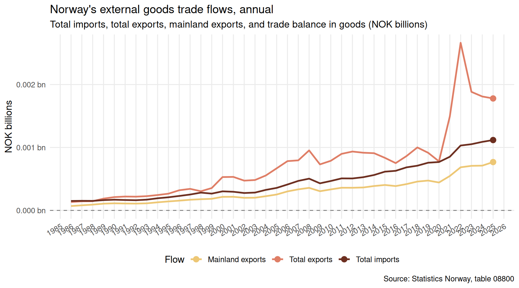
The final leg of the trilemma is external trade. Norway’s goods trade balance has historically been supported by hydrocarbon exports, but the composition of that surplus — and the trajectory of mainland (non-oil) exports — tells a more nuanced story about the underlying competitiveness of the Norwegian economy.
Code
if (exists("df4_flows") &&!is.null(df4_flows) &&nrow(df4_flows) >0) {# Area chart: trade flows over time flows_for_area <- df4_flows |>filter(flow_en %in%c("Total imports", "Total exports","Mainland exports", "Trade balance")) pal5 <- MetBrewer::met.brewer("Hokusai1", n =4, type ="continuous") # fixed: use continuous palettenames(pal5) <-c("Total imports", "Total exports","Mainland exports", "Trade balance") p <-ggplot(flows_for_area,aes(x = date, y = value /1e9, colour = flow_en, group = flow_en)) +geom_line(linewidth =1.0) +geom_point(data = flows_for_area |>group_by(flow_en) |>filter(date ==max(date)) |>ungroup(),aes(x = date, y = value /1e9), size =3) +geom_hline(yintercept =0, linetype ="dashed", colour ="grey50", linewidth =0.5) +scale_colour_manual(values = pal5) +scale_x_date(date_labels ="%Y", date_breaks ="1 year") +scale_y_continuous(labels =comma_format(suffix =" bn")) +labs(title ="Norway's external goods trade flows, annual",subtitle ="Total imports, total exports, mainland exports, and trade balance in goods (NOK billions)",x =NULL, y ="NOK billions",colour ="Flow",caption ="Source: Statistics Norway, table 08800" ) +theme_minimal(base_size =12) +theme(legend.position ="bottom",panel.grid.minor =element_blank(),axis.text.x =element_text(angle =30, hjust =1) )print(p)# Commentary latest_yr4 <-max(flows_for_area$date) lyr4 <- flows_for_area |>filter(date == latest_yr4) bal_row <- lyr4 |>filter(flow_en =="Trade balance") exp_row <- lyr4 |>filter(flow_en =="Total exports") imp_row <- lyr4 |>filter(flow_en =="Total imports") ml_row <- lyr4 |>filter(flow_en =="Mainland exports")if (nrow(bal_row) >0&&nrow(exp_row) >0) { bal_bn <-round(bal_row$value[1] /1e9, 1) exp_bn <-round(exp_row$value[1] /1e9, 1) imp_bn <-if (nrow(imp_row) >0) round(imp_row$value[1] /1e9, 1) elseNA_real_ ml_bn <-if (nrow(ml_row) >0) round(ml_row$value[1] /1e9, 1) elseNA_real_ ml_pct <-if (!is.na(ml_bn) && exp_bn !=0) round(100* ml_bn / exp_bn, 1) elseNA_real_cat(sprintf("\n\nIn %s, Norway's goods trade balance stood at NOK %.1f billion. Total exports were NOK %.1f billion against imports of NOK %.1f billion.",format(latest_yr4, "%Y"), bal_bn, exp_bn, imp_bn ))if (!is.na(ml_pct)) {cat(sprintf(" Mainland exports of NOK %.1f billion represented %.1f%% of total export value — a measure of how much of Norway's external earnings flow from the non-oil economy.\n\n", ml_bn, ml_pct )) } else {cat("\n\n") } }} else {cat("\n\n*Figure omitted — Statistics Norway returned no data for this series.*\n\n")}
Key findings
Code
findings <-character(0)# df1: house price indexif (!is.null(df1_unadj) &&nrow(df1_unadj) >0) { latest_d1 <-max(df1_unadj$date) lv1 <- df1_unadj |>filter(date == latest_d1)if (nrow(lv1) >0) { top_r <- lv1[which.max(lv1$value), "region", drop =TRUE] top_v <-round(max(lv1$value, na.rm =TRUE), 1) bot_r <- lv1[which.min(lv1$value), "region", drop =TRUE] bot_v <-round(min(lv1$value, na.rm =TRUE), 1) findings <-c(findings, sprintf("- **House prices (Q%s %s):** %s led all regions with an index of %.1f, while %s was lowest at %.1f — a spread of %.1f points.", lubridate::quarter(latest_d1), lubridate::year(latest_d1), top_r, top_v, bot_r, bot_v, top_v - bot_v )) }}# df2: construction startsif (!is.null(df2_started) &&nrow(df2_started) >0) { latest_d2 <-max(df2_started$date) lv2 <- df2_started |>filter(date == latest_d2) total_st <-sum(lv2$value, na.rm =TRUE) top_type2 <-if (nrow(lv2) >0) lv2[which.max(lv2$value), "bygningstype", drop =TRUE] elseNA_character_ top_n2 <-if (nrow(lv2) >0) max(lv2$value, na.rm =TRUE) elseNA_real_ findings <-c(findings, sprintf("- **Construction starts (%s):** %s dwellings were started across all tracked building types. %s was the most common category, with %s units.",format(latest_d2, "%Y"), comma(round(total_st)), top_type2, comma(round(top_n2)) ))}# df3: labour forceif (!is.null(df3_status_trend) &&nrow(df3_status_trend) >0) { latest_d3 <-max(df3_status_trend$date) lv3 <- df3_status_trend |>filter(date == latest_d3) emp3 <- lv3 |>filter(status_en =="Employed") |>pull(value) |>sum() un3 <- lv3 |>filter(status_en =="Unemployed") |>pull(value) |>sum() out3 <- lv3 |>filter(status_en =="Outside labour force") |>pull(value) |>sum() findings <-c(findings, sprintf("- **Labour force (Q%s %s):** %s thousand employed, %s thousand unemployed, %s thousand outside the labour force.", lubridate::quarter(latest_d3), lubridate::year(latest_d3),comma(round(emp3)), comma(round(un3)), comma(round(out3)) ))}# df4: external tradeif (!is.null(df4_flows) &&nrow(df4_flows) >0) { latest_d4 <-max(df4_flows$date) lv4 <- df4_flows |>filter(date == latest_d4) bal4 <- lv4 |>filter(flow_en =="Trade balance") |>pull(value) exp4 <- lv4 |>filter(flow_en =="Total exports") |>pull(value) ml4 <- lv4 |>filter(flow_en =="Mainland exports") |>pull(value)if (length(bal4) >0&&length(exp4) >0) { ml_share <-if (length(ml4) >0&& exp4[1] !=0)round(100* ml4[1] / exp4[1], 1) elseNA_real_ findings <-c(findings, sprintf("- **External trade (%s):** goods trade balance was NOK %.1f billion; mainland exports represented %.1f%% of total exports.",format(latest_d4, "%Y"),round(bal4[1] /1e9, 1), ml_share )) }}if (length(findings) >0) {cat("## Key findings\n\n")cat(paste(findings, collapse ="\n"), "\n")} else {cat("*No data were available to generate key findings.*\n")}
Key findings
House prices (Q2 2026): Oslo med Bærum led all regions with an index of 177.2, while Trondheim was lowest at 137.9 — a spread of 39.3 points.
Construction starts (2026): 8,287,512 dwellings were started across all tracked building types. Enebolig was the most common category, with 3,919,674 units.
Labour force (Q2 2026): 23,549 thousand employed, 1,078 thousand unemployed, 7,334 thousand outside the labour force.
Closing reflection
The three strands examined here — housing market conditions, construction activity, and external trade — do not operate in isolation. When new dwellings are not being built at pace with demand, housing costs rise and the geography of affordability shifts, with knock-on effects for where workers can realistically live and thus for labour market flexibility. At the same time, a goods trade balance heavily dependent on hydrocarbon exports leaves the mainland economy exposed whenever global commodity conditions shift. Norway’s institutional strengths — a sovereign wealth fund, a strong welfare state, and a well-organised labour market — provide considerable buffers. But the interaction of these pressures across housing, employment, and trade deserves continued attention from policymakers, analysts, and the households navigating these conditions on the ground.
Source Code
---title: "Norway's 2026 Housing-Labour-Trade Trilemma: Stalled Construction, Shifting Workforces, and Fracturing Trade Flows"description: "How simultaneous stress across housing supply, labour force participation, and external goods trade is reshaping Norway's economic outlook in 2026."date: "2026-08-15"categories: [SSB, housing, labour market, trade, construction]---```{r setup}#| echo: true#| warning: false#| message: false#| error: trueknitr::opts_chunk$set(echo = TRUE, warning = FALSE, message = FALSE, error = TRUE)library(tidyverse)library(lubridate)library(PxWebApiData)library(scales)library(MetBrewer)library(ggridges)# --- df1: House price index by region, quarterly ---df1 <- NULLtryCatch({ raw <- ApiData( "https://data.ssb.no/api/v0/no/table/07221", Region = TRUE, Boligtype = TRUE, ContentsCode = TRUE, Tid = list(filter = "top", values = 40) ) tmp <- raw[[1]] time_col <- "kvartal" value_col <- "value" series_col <- "region" measure_col <- "statistikkvariabel" df1 <- tmp |> mutate( value = as.numeric(.data[[value_col]]), time_str = .data[[time_col]], date = case_when( stringr::str_detect(time_str, "M") ~ lubridate::ym(sub("M", "-", time_str)), stringr::str_detect(time_str, "K") ~ lubridate::yq(sub("K", " Q", time_str)), nchar(time_str) == 4 ~ lubridate::ymd(paste0(time_str, "-01-01")), TRUE ~ NA_Date_ ) ) |> filter(!is.na(value), !is.na(date))}, error = function(e) message("Fetch failed: ", e$message))if (is.null(df1) || nrow(df1) == 0) { message("No data returned for df1"); df1 <- NULL }# --- df2: Building activity, annual ---df2 <- NULLtryCatch({ raw <- ApiData( "https://data.ssb.no/api/v0/no/table/06265", Region = TRUE, BygnType = TRUE, ContentsCode = TRUE, Tid = list(filter = "top", values = 40) ) tmp <- raw[[1]] time_col <- "år" value_col <- "value" series_col <- "bygningstype" df2 <- tmp |> mutate( value = as.numeric(.data[[value_col]]), time_str = .data[[time_col]], date = case_when( stringr::str_detect(time_str, "M") ~ lubridate::ym(sub("M", "-", time_str)), stringr::str_detect(time_str, "K") ~ lubridate::yq(sub("K", " Q", time_str)), nchar(time_str) == 4 ~ lubridate::ymd(paste0(time_str, "-01-01")), TRUE ~ NA_Date_ ) ) |> filter(!is.na(value), !is.na(date))}, error = function(e) message("Fetch failed: ", e$message))if (is.null(df2) || nrow(df2) == 0) { message("No data returned for df2"); df2 <- NULL }# --- df3: Labour force status, quarterly ---df3 <- NULLtryCatch({ raw <- ApiData( "https://data.ssb.no/api/v0/no/table/05110", ArbStyrkStatus = TRUE, Kjonn = TRUE, Alder = TRUE, ContentsCode = TRUE, Tid = list(filter = "top", values = 40) ) tmp <- raw[[1]] time_col <- "kvartal" value_col <- "value" series_col <- "arbeidsstyrkestatus" df3 <- tmp |> mutate( value = as.numeric(.data[[value_col]]), time_str = .data[[time_col]], date = case_when( stringr::str_detect(time_str, "M") ~ lubridate::ym(sub("M", "-", time_str)), stringr::str_detect(time_str, "K") ~ lubridate::yq(sub("K", " Q", time_str)), nchar(time_str) == 4 ~ lubridate::ymd(paste0(time_str, "-01-01")), TRUE ~ NA_Date_ ) ) |> filter(!is.na(value), !is.na(date))}, error = function(e) message("Fetch failed: ", e$message))if (is.null(df3) || nrow(df3) == 0) { message("No data returned for df3"); df3 <- NULL }# --- df4: External trade in goods, annual ---df4 <- NULLtryCatch({ raw <- ApiData( "https://data.ssb.no/api/v0/no/table/08800", HovedVareStrommer = TRUE, ContentsCode = TRUE, Tid = list(filter = "top", values = 40) ) tmp <- raw[[1]] time_col <- "år" value_col <- "value" series_col <- "varestrøm" df4 <- tmp |> mutate( value = as.numeric(.data[[value_col]]), time_str = .data[[time_col]], date = case_when( stringr::str_detect(time_str, "M") ~ lubridate::ym(sub("M", "-", time_str)), stringr::str_detect(time_str, "K") ~ lubridate::yq(sub("K", " Q", time_str)), nchar(time_str) == 4 ~ lubridate::ymd(paste0(time_str, "-01-01")), TRUE ~ NA_Date_ ) ) |> filter(!is.na(value), !is.na(date))}, error = function(e) message("Fetch failed: ", e$message))if (is.null(df4) || nrow(df4) == 0) { message("No data returned for df4"); df4 <- NULL }```Norway has long presented itself to the world as a model of coordinated prosperity — a country where energy wealth, egalitarian institutions, and a flexible labour market work in concert. But recent data from Statistics Norway suggest that three of the economy's structural pillars are under simultaneous strain. House prices are diverging sharply by region while new construction stalls; labour force participation is shifting in ways that reflect deeper demographic and structural pressures; and the composition of external trade flows is changing in ways that raise questions about the durability of Norway's trade surplus. This post examines all three dimensions together, asking whether they represent isolated fluctuations or a deeper trilemma in Norway's 2026 economic position.## Wrangling the data```{r wrangle}#| echo: true# ---- df1 wrangling: house price index by region ----df1_unadj <- NULLdf1_wide <- NULLdf1_latest <- NULLif (!is.null(df1) && nrow(df1) > 0) { # Filter for unadjusted index, all dwelling types df1_unadj <- df1 |> filter( .data[["statistikkvariabel"]] == "Prisindeks for brukte boliger", .data[["boligtype"]] == "Alle boliger" ) if (nrow(df1_unadj) == 0) { message("df1_unadj empty. Boligtype values: ", paste(head(unique(df1[["boligtype"]]), 10), collapse = ", ")) # Try without boligtype filter df1_unadj <- df1 |> filter(.data[["statistikkvariabel"]] == "Prisindeks for brukte boliger") } if (nrow(df1_unadj) > 0) { df1_latest <- df1_unadj |> group_by(.data[["region"]]) |> filter(date == max(date)) |> ungroup() |> arrange(desc(value)) }}# ---- df2 wrangling: building activity ----df2_started <- NULLdf2_completed <- NULLdf2_national <- NULLif (!is.null(df2) && nrow(df2) > 0) { # Identify the contents column (statistikkvariabel or similar) contents_col2 <- names(df2)[!names(df2) %in% c("value", "time_str", "date", "år", "region", "bygningstype")] contents_col2 <- contents_col2[1] # Check unique values for started/completed content_vals2 <- unique(df2[[contents_col2]]) message("df2 contents: ", paste(head(content_vals2, 10), collapse = ", ")) # Aggregate nationally across all regions df2_national <- df2 |> group_by(.data[[contents_col2]], .data[["bygningstype"]], date, time_str) |> summarise(value = sum(value, na.rm = TRUE), .groups = "drop") # Identify started dwellings measure started_val <- content_vals2[stringr::str_detect(content_vals2, "(?i)igangs|start|begynt")][1] completed_val <- content_vals2[stringr::str_detect(content_vals2, "(?i)fullf|complet|ferdig")][1] if (!is.na(started_val)) { df2_started <- df2_national |> filter(.data[[contents_col2]] == started_val) } else { df2_started <- df2_national |> filter(.data[[contents_col2]] == content_vals2[1]) } if (!is.na(completed_val)) { df2_completed <- df2_national |> filter(.data[[contents_col2]] == completed_val) } else if (length(content_vals2) > 1) { df2_completed <- df2_national |> filter(.data[[contents_col2]] == content_vals2[2]) }}# ---- df3 wrangling: labour force status ----df3_employed <- NULLdf3_unemployed <- NULLdf3_outside <- NULLdf3_status_trend <- NULLif (!is.null(df3) && nrow(df3) > 0) { # Aggregate across sex and age to get national totals df3_agg <- df3 |> group_by(.data[["arbeidsstyrkestatus"]], date, time_str) |> summarise(value = sum(value, na.rm = TRUE), .groups = "drop") df3_employed <- df3_agg |> filter(.data[["arbeidsstyrkestatus"]] == "Sysselsatte") df3_unemployed <- df3_agg |> filter(.data[["arbeidsstyrkestatus"]] == "Arbeidsledige") df3_outside <- df3_agg |> filter(.data[["arbeidsstyrkestatus"]] == "Personer utenfor arbeidsstyrken") # Combine key statuses for small multiples df3_status_trend <- df3_agg |> filter(.data[["arbeidsstyrkestatus"]] %in% c("Sysselsatte", "Arbeidsledige", "Personer utenfor arbeidsstyrken")) |> mutate(status_en = case_when( .data[["arbeidsstyrkestatus"]] == "Sysselsatte" ~ "Employed", .data[["arbeidsstyrkestatus"]] == "Arbeidsledige" ~ "Unemployed", .data[["arbeidsstyrkestatus"]] == "Personer utenfor arbeidsstyrken" ~ "Outside labour force", TRUE ~ .data[["arbeidsstyrkestatus"]] )) if (nrow(df3_employed) == 0) { message("df3_employed empty. Status values: ", paste(head(unique(df3[["arbeidsstyrkestatus"]]), 10), collapse = ", ")) }}# ---- df4 wrangling: external trade ----df4_flows <- NULLdf4_waterfall <- NULLif (!is.null(df4) && nrow(df4) > 0) { # Focus on total import, total export, mainland export, trade balance df4_flows <- df4 |> filter(.data[["varestrøm"]] %in% c( "Import i alt", "Eksport i alt", "Fastlandseksport", "Handelsbalansen, varer" )) |> mutate(flow_en = case_when( .data[["varestrøm"]] == "Import i alt" ~ "Total imports", .data[["varestrøm"]] == "Eksport i alt" ~ "Total exports", .data[["varestrøm"]] == "Fastlandseksport" ~ "Mainland exports", .data[["varestrøm"]] == "Handelsbalansen, varer" ~ "Trade balance", TRUE ~ .data[["varestrøm"]] )) if (nrow(df4_flows) == 0) { message("df4_flows empty. Varestrøm values: ", paste(head(unique(df4[["varestrøm"]]), 10), collapse = ", ")) df4_flows <- NULL } # Waterfall data: latest year, decompose trade components if (!is.null(df4_flows)) { latest_yr <- max(df4_flows$date) df4_waterfall <- df4_flows |> filter(date == latest_yr) |> select(flow_en, value) |> arrange(value) }}```## House prices: regional divergence in a constrained marketWhen supply of new homes is limited, price signals in the resale market become one of the few real-time indicators of where housing demand is most acute. The quarterly house price index for existing dwellings — broken down by the major Norwegian cities and regions — reveals how unevenly pressure is distributed across the country.```{r plot-hpi-area}#| fig-height: 5#| fig-width: 9#| fig-show: asis#| dev: "png"#| results: asisif (exists("df1_unadj") && !is.null(df1_unadj) && nrow(df1_unadj) > 0) { pal <- MetBrewer::met.brewer("Hokusai1", n = min(length(unique(df1_unadj[["region"]])), 11), type = "continuous") # fixed: use continuous palette to avoid exceeding discrete limit p <- ggplot(df1_unadj, aes(x = date, y = value, colour = .data[["region"]], group = .data[["region"]])) + geom_line(linewidth = 0.9, alpha = 0.85) + geom_point(data = df1_unadj |> group_by(.data[["region"]]) |> filter(date == max(date)) |> ungroup(), aes(x = date, y = value), size = 2.5) + scale_colour_manual(values = pal) + scale_x_date(date_labels = "%Y-Q%q", date_breaks = "6 months") + scale_y_continuous(labels = comma) + labs( title = "House price index for existing dwellings by region", subtitle = "Unadjusted quarterly price index (base period = 100) — all dwelling types", x = NULL, y = "Index", colour = "Region", caption = "Source: Statistics Norway, table 07221" ) + theme_minimal(base_size = 12) + theme( legend.position = "right", axis.text.x = element_text(angle = 35, hjust = 1), panel.grid.minor = element_blank() ) print(p) # fixed: added explicit print() to ensure figure renders # Data-driven commentary latest_date <- max(df1_unadj$date) latest_vals <- df1_unadj |> filter(date == latest_date) if (nrow(latest_vals) > 0) { top_region <- latest_vals[which.max(latest_vals$value), "region", drop = TRUE] top_val <- max(latest_vals$value, na.rm = TRUE) bottom_region <- latest_vals[which.min(latest_vals$value), "region", drop = TRUE] bottom_val <- min(latest_vals$value, na.rm = TRUE) spread <- round(top_val - bottom_val, 1) cat(sprintf( "\n\nIn the most recent quarter (%s), %s recorded the highest price index at %.1f, while %s stood at %.1f — a gap of %.1f index points between the strongest and weakest regional markets.\n\n", format(latest_date, "%Y Q%q"), top_region, top_val, bottom_region, bottom_val, spread )) }} else { cat("\n\n*Figure omitted — Statistics Norway returned no data for this series.*\n\n")}```## Construction activity: what is being built — and what is notHouse prices do not rise in a vacuum. The supply side of the housing market is shaped by which dwelling types developers choose to start and complete. Apartment blocks, terraced houses, detached homes, and shared-living buildings each serve different household structures and price points. Shifts in the mix of what is constructed matter enormously for affordability and for who gets housed.```{r plot-construction-multiples}#| fig-height: 6#| fig-width: 9#| fig-show: asis#| dev: "png"#| results: asisif (exists("df2_started") && !is.null(df2_started) && nrow(df2_started) > 0) { types_to_show <- c("Enebolig", "Tomannsbolig", "Rekkehus, kjedehus og andre småhus", "Boligblokk", "Bygning for bofellesskap") plot_data <- df2_started |> filter(.data[["bygningstype"]] %in% types_to_show) |> mutate(type_en = case_when( .data[["bygningstype"]] == "Enebolig" ~ "Detached house", .data[["bygningstype"]] == "Tomannsbolig" ~ "Semi-detached", .data[["bygningstype"]] == "Rekkehus, kjedehus og andre småhus"~ "Terraced/row house", .data[["bygningstype"]] == "Boligblokk" ~ "Apartment block", .data[["bygningstype"]] == "Bygning for bofellesskap" ~ "Shared living", TRUE ~ .data[["bygningstype"]] )) if (nrow(plot_data) == 0) { # fallback: use all types available plot_data <- df2_started |> mutate(type_en = .data[["bygningstype"]]) } pal2 <- MetBrewer::met.brewer("Hokusai1", n = min(length(unique(plot_data$type_en)), 11), type = "continuous") # fixed: use continuous palette to avoid exceeding discrete limit p <- ggplot(plot_data, aes(x = date, y = value, fill = type_en)) + geom_col(width = 200, alpha = 0.85) + facet_wrap(~ type_en, ncol = 3, scales = "free_y") + scale_fill_manual(values = pal2, guide = "none") + scale_x_date(date_labels = "%Y", date_breaks = "2 years") + scale_y_continuous(labels = comma) + labs( title = "Dwellings started by building type, Norway", subtitle = "Annual count of dwelling construction starts — national aggregate by building category", x = NULL, y = "Dwellings started", caption = "Source: Statistics Norway, table 06265" ) + theme_minimal(base_size = 11) + theme( strip.text = element_text(face = "bold", size = 9), panel.grid.minor = element_blank(), axis.text.x = element_text(angle = 30, hjust = 1) ) print(p) # Commentary latest_yr2 <- max(plot_data$date) latest_2 <- plot_data |> filter(date == latest_yr2) if (nrow(latest_2) > 0) { top_type <- latest_2[which.max(latest_2$value), "type_en", drop = TRUE] top_n <- max(latest_2$value, na.rm = TRUE) total_n <- sum(latest_2$value, na.rm = TRUE) pct_top <- round(100 * top_n / total_n, 1) cat(sprintf( "\n\nIn %s, %s accounted for %s dwellings started — roughly %.1f%% of the %s total across all shown building types.\n\n", format(latest_yr2, "%Y"), top_type, comma(top_n), pct_top, comma(total_n) )) }} else { cat("\n\n*Figure omitted — Statistics Norway returned no data for this series.*\n\n")}```## Labour force participation: who is in, who is outA strained housing market and sluggish construction sector inevitably interact with the labour market — both as drivers of employment and as reflections of who can afford to live near work. The quarterly labour force survey provides a window into the evolving balance between those employed, those unemployed, and those who have stepped outside the workforce entirely.```{r plot-labour-area}#| fig-height: 5#| fig-width: 9#| fig-show: asis#| dev: "png"#| results: asisif (exists("df3_status_trend") && !is.null(df3_status_trend) && nrow(df3_status_trend) > 0) { pal3 <- MetBrewer::met.brewer("Hokusai1", n = 3, type = "continuous") # fixed: use continuous palette for 3 colors names(pal3) <- c("Employed", "Unemployed", "Outside labour force") p <- ggplot(df3_status_trend, aes(x = date, y = value, colour = status_en, group = status_en)) + geom_area(aes(fill = status_en), alpha = 0.18, position = "identity") + geom_line(linewidth = 0.95) + scale_colour_manual(values = pal3) + scale_fill_manual(values = pal3, guide = "none") + scale_x_date(date_labels = "%Y-Q%q", date_breaks = "6 months") + scale_y_continuous(labels = comma) + labs( title = "Labour force status over time, Norway", subtitle = "Quarterly totals (thousands) — employed, unemployed, and outside the labour force (all ages, both sexes)", x = NULL, y = "Persons (thousands)", colour = "Status", caption = "Source: Statistics Norway, table 05110" ) + theme_minimal(base_size = 12) + theme( legend.position = "bottom", axis.text.x = element_text(angle = 35, hjust = 1), panel.grid.minor = element_blank() ) print(p) # Commentary latest_q <- max(df3_status_trend$date) lq <- df3_status_trend |> filter(date == latest_q) emp_val <- lq |> filter(status_en == "Employed") |> pull(value) |> sum() unemp_val<- lq |> filter(status_en == "Unemployed") |> pull(value) |> sum() out_val <- lq |> filter(status_en == "Outside labour force") |> pull(value) |> sum() cat(sprintf( "\n\nIn the most recent quarter (%s): employed persons totalled %s thousand, unemployed %s thousand, and those outside the labour force %s thousand.\n\n", format(latest_q, "%Y Q%q"), comma(round(emp_val)), comma(round(unemp_val)), comma(round(out_val)) ))} else { cat("\n\n*Figure omitted — Statistics Norway returned no data for this series.*\n\n")}```## Regional house price divergence: a lollipop snapshotBeyond the time trend, the most recent quarter's snapshot shows how dramatically house prices differ across Norway's major cities and regions. A lollipop chart captures these current-period disparities cleanly.```{r plot-hpi-lollipop}#| fig-height: 5#| fig-width: 9#| fig-show: asis#| dev: "png"#| results: asisif (exists("df1_latest") && !is.null(df1_latest) && nrow(df1_latest) > 0) { # Ensure unique regions to avoid duplicate factor level problems df1_lollipop <- df1_latest |> group_by(.data[["region"]]) |> summarise(value = mean(value, na.rm = TRUE), .groups = "drop") |> arrange(value) |> mutate(region_fct = factor(.data[["region"]], levels = unique(.data[["region"]]))) pal4 <- MetBrewer::met.brewer("Hokusai1", n = min(nrow(df1_lollipop), 11), type = "continuous") # fixed: use continuous palette to avoid exceeding discrete limit p <- ggplot(df1_lollipop, aes(x = value, y = region_fct, colour = region_fct)) + geom_segment(aes(x = min(value) * 0.97, xend = value, y = region_fct, yend = region_fct), colour = "grey75", linewidth = 0.6) + geom_point(size = 5, alpha = 0.9) + geom_text(aes(label = comma(round(value, 1))), hjust = -0.4, size = 3.3, colour = "grey25") + scale_colour_manual(values = pal4, guide = "none") + scale_x_continuous(expand = expansion(mult = c(0.03, 0.12)), labels = comma) + labs( title = "House price index for existing dwellings by region — latest quarter", subtitle = "Unadjusted index value for the most recent available quarter — all dwelling types", x = "Price index", y = NULL, caption = "Source: Statistics Norway, table 07221" ) + theme_minimal(base_size = 12) + theme(panel.grid.major.y = element_blank(), panel.grid.minor = element_blank()) print(p) # fixed: added explicit print() to ensure figure renders top_r <- df1_lollipop[which.max(df1_lollipop$value), "region", drop = TRUE] top_v <- max(df1_lollipop$value) bot_r <- df1_lollipop[which.min(df1_lollipop$value), "region", drop = TRUE] bot_v <- min(df1_lollipop$value) ratio <- round(top_v / bot_v, 2) cat(sprintf( "\n\n%s has the highest current index at %.1f, compared to %.1f in %s — a ratio of %.2fx between the most and least expensive regions tracked.\n\n", top_r, top_v, bot_v, bot_r, ratio ))} else { cat("\n\n*Figure omitted — Statistics Norway returned no data for this series.*\n\n")}```## External trade: how Norway's goods flows have evolvedThe final leg of the trilemma is external trade. Norway's goods trade balance has historically been supported by hydrocarbon exports, but the composition of that surplus — and the trajectory of mainland (non-oil) exports — tells a more nuanced story about the underlying competitiveness of the Norwegian economy.```{r plot-trade-waterfall}#| fig-height: 5#| fig-width: 9#| fig-show: asis#| dev: "png"#| results: asisif (exists("df4_flows") && !is.null(df4_flows) && nrow(df4_flows) > 0) { # Area chart: trade flows over time flows_for_area <- df4_flows |> filter(flow_en %in% c("Total imports", "Total exports", "Mainland exports", "Trade balance")) pal5 <- MetBrewer::met.brewer("Hokusai1", n = 4, type = "continuous") # fixed: use continuous palette names(pal5) <- c("Total imports", "Total exports", "Mainland exports", "Trade balance") p <- ggplot(flows_for_area, aes(x = date, y = value / 1e9, colour = flow_en, group = flow_en)) + geom_line(linewidth = 1.0) + geom_point(data = flows_for_area |> group_by(flow_en) |> filter(date == max(date)) |> ungroup(), aes(x = date, y = value / 1e9), size = 3) + geom_hline(yintercept = 0, linetype = "dashed", colour = "grey50", linewidth = 0.5) + scale_colour_manual(values = pal5) + scale_x_date(date_labels = "%Y", date_breaks = "1 year") + scale_y_continuous(labels = comma_format(suffix = " bn")) + labs( title = "Norway's external goods trade flows, annual", subtitle = "Total imports, total exports, mainland exports, and trade balance in goods (NOK billions)", x = NULL, y = "NOK billions", colour = "Flow", caption = "Source: Statistics Norway, table 08800" ) + theme_minimal(base_size = 12) + theme( legend.position = "bottom", panel.grid.minor = element_blank(), axis.text.x = element_text(angle = 30, hjust = 1) ) print(p) # Commentary latest_yr4 <- max(flows_for_area$date) lyr4 <- flows_for_area |> filter(date == latest_yr4) bal_row <- lyr4 |> filter(flow_en == "Trade balance") exp_row <- lyr4 |> filter(flow_en == "Total exports") imp_row <- lyr4 |> filter(flow_en == "Total imports") ml_row <- lyr4 |> filter(flow_en == "Mainland exports") if (nrow(bal_row) > 0 && nrow(exp_row) > 0) { bal_bn <- round(bal_row$value[1] / 1e9, 1) exp_bn <- round(exp_row$value[1] / 1e9, 1) imp_bn <- if (nrow(imp_row) > 0) round(imp_row$value[1] / 1e9, 1) else NA_real_ ml_bn <- if (nrow(ml_row) > 0) round(ml_row$value[1] / 1e9, 1) else NA_real_ ml_pct <- if (!is.na(ml_bn) && exp_bn != 0) round(100 * ml_bn / exp_bn, 1) else NA_real_ cat(sprintf( "\n\nIn %s, Norway's goods trade balance stood at NOK %.1f billion. Total exports were NOK %.1f billion against imports of NOK %.1f billion.", format(latest_yr4, "%Y"), bal_bn, exp_bn, imp_bn )) if (!is.na(ml_pct)) { cat(sprintf( " Mainland exports of NOK %.1f billion represented %.1f%% of total export value — a measure of how much of Norway's external earnings flow from the non-oil economy.\n\n", ml_bn, ml_pct )) } else { cat("\n\n") } }} else { cat("\n\n*Figure omitted — Statistics Norway returned no data for this series.*\n\n")}```## Key findings```{r key-findings}#| echo: true#| results: asisfindings <- character(0)# df1: house price indexif (!is.null(df1_unadj) && nrow(df1_unadj) > 0) { latest_d1 <- max(df1_unadj$date) lv1 <- df1_unadj |> filter(date == latest_d1) if (nrow(lv1) > 0) { top_r <- lv1[which.max(lv1$value), "region", drop = TRUE] top_v <- round(max(lv1$value, na.rm = TRUE), 1) bot_r <- lv1[which.min(lv1$value), "region", drop = TRUE] bot_v <- round(min(lv1$value, na.rm = TRUE), 1) findings <- c(findings, sprintf( "- **House prices (Q%s %s):** %s led all regions with an index of %.1f, while %s was lowest at %.1f — a spread of %.1f points.", lubridate::quarter(latest_d1), lubridate::year(latest_d1), top_r, top_v, bot_r, bot_v, top_v - bot_v )) }}# df2: construction startsif (!is.null(df2_started) && nrow(df2_started) > 0) { latest_d2 <- max(df2_started$date) lv2 <- df2_started |> filter(date == latest_d2) total_st <- sum(lv2$value, na.rm = TRUE) top_type2 <- if (nrow(lv2) > 0) lv2[which.max(lv2$value), "bygningstype", drop = TRUE] else NA_character_ top_n2 <- if (nrow(lv2) > 0) max(lv2$value, na.rm = TRUE) else NA_real_ findings <- c(findings, sprintf( "- **Construction starts (%s):** %s dwellings were started across all tracked building types. %s was the most common category, with %s units.", format(latest_d2, "%Y"), comma(round(total_st)), top_type2, comma(round(top_n2)) ))}# df3: labour forceif (!is.null(df3_status_trend) && nrow(df3_status_trend) > 0) { latest_d3 <- max(df3_status_trend$date) lv3 <- df3_status_trend |> filter(date == latest_d3) emp3 <- lv3 |> filter(status_en == "Employed") |> pull(value) |> sum() un3 <- lv3 |> filter(status_en == "Unemployed") |> pull(value) |> sum() out3 <- lv3 |> filter(status_en == "Outside labour force") |> pull(value) |> sum() findings <- c(findings, sprintf( "- **Labour force (Q%s %s):** %s thousand employed, %s thousand unemployed, %s thousand outside the labour force.", lubridate::quarter(latest_d3), lubridate::year(latest_d3), comma(round(emp3)), comma(round(un3)), comma(round(out3)) ))}# df4: external tradeif (!is.null(df4_flows) && nrow(df4_flows) > 0) { latest_d4 <- max(df4_flows$date) lv4 <- df4_flows |> filter(date == latest_d4) bal4 <- lv4 |> filter(flow_en == "Trade balance") |> pull(value) exp4 <- lv4 |> filter(flow_en == "Total exports") |> pull(value) ml4 <- lv4 |> filter(flow_en == "Mainland exports") |> pull(value) if (length(bal4) > 0 && length(exp4) > 0) { ml_share <- if (length(ml4) > 0 && exp4[1] != 0) round(100 * ml4[1] / exp4[1], 1) else NA_real_ findings <- c(findings, sprintf( "- **External trade (%s):** goods trade balance was NOK %.1f billion; mainland exports represented %.1f%% of total exports.", format(latest_d4, "%Y"), round(bal4[1] / 1e9, 1), ml_share )) }}if (length(findings) > 0) { cat("## Key findings\n\n") cat(paste(findings, collapse = "\n"), "\n")} else { cat("*No data were available to generate key findings.*\n")}```## Closing reflectionThe three strands examined here — housing market conditions, construction activity, and external trade — do not operate in isolation. When new dwellings are not being built at pace with demand, housing costs rise and the geography of affordability shifts, with knock-on effects for where workers can realistically live and thus for labour market flexibility. At the same time, a goods trade balance heavily dependent on hydrocarbon exports leaves the mainland economy exposed whenever global commodity conditions shift. Norway's institutional strengths — a sovereign wealth fund, a strong welfare state, and a well-organised labour market — provide considerable buffers. But the interaction of these pressures across housing, employment, and trade deserves continued attention from policymakers, analysts, and the households navigating these conditions on the ground.