Monthly consumer price data and annual national accounts reveal how diverging price pressures across spending categories are reshaping Norwegian household consumption in real terms.
Norway has long enjoyed a reputation for economic resilience — sustained by oil revenues, strong institutions, and a robust welfare state. But within that broader stability, a more nuanced story is playing out at the household level. Consumer prices across different spending categories have been moving at sharply different speeds, while the volume of what households actually buy has shown a more complicated trajectory. The question is whether the composition of inflation — not just its overall level — is quietly reordering Norwegian household budgets in ways the headline numbers obscure.
This post traces that divergence through two complementary datasets: monthly consumer price index readings across major spending categories, and annual national accounts data on household and public consumption in both current and fixed prices.
Code
# ── df1 wrangling ──────────────────────────────────────────────────────────────df1_annual_change <-NULLdf1_heatmap <-NULLdf1_latest_lollipop <-NULLdf1_index <-NULLif (!is.null(df1) &&nrow(df1) >0) { series_col1 <-"konsumgruppe" measure_col1 <-"statistikkvariabel"# 12-month change for all consumption groups df1_annual_change <- df1 |>filter(.data[[measure_col1]] =="12-måneders endring (prosent)") |>filter(.data[[series_col1]] !="Totalindeks") |>mutate(group_short =case_when( .data[[series_col1]] =="Matvarer og alkoholfrie drikkevarer"~"Food & non-alc.", .data[[series_col1]] =="Alkoholholdige drikkevarer og tobakk"~"Alcohol & tobacco", .data[[series_col1]] =="Klær og skotøy"~"Clothing & footwear", .data[[series_col1]] =="Bolig, lys og brensel"~"Housing, energy", .data[[series_col1]] =="Møbler, husholdningsartikler og vedlikehold av innbo"~"Furniture & HH goods", .data[[series_col1]] =="Helsepleie"~"Healthcare", .data[[series_col1]] =="Transport"~"Transport", .data[[series_col1]] =="Post- og teletjenester"~"Post & telecom", .data[[series_col1]] =="Kultur og fritid"~"Culture & leisure",TRUE~ .data[[series_col1]] ))# For heatmap: monthly readings over time per group df1_heatmap <- df1_annual_change |>filter(!is.na(value))# Latest month lollipopif (nrow(df1_annual_change) >0) { latest_date <-max(df1_annual_change$date, na.rm =TRUE) df1_latest_lollipop <- df1_annual_change |>filter(date == latest_date) |>arrange(value) }# CPI index level for Totalindeks vs selected groups df1_index <- df1 |>filter(.data[[measure_col1]] =="Konsumprisindeks (2015=100)") |>filter(.data[[series_col1]] %in%c("Totalindeks","Bolig, lys og brensel","Matvarer og alkoholfrie drikkevarer","Transport","Kultur og fritid" )) |>mutate(group_short =case_when( .data[[series_col1]] =="Totalindeks"~"Total CPI", .data[[series_col1]] =="Bolig, lys og brensel"~"Housing & energy", .data[[series_col1]] =="Matvarer og alkoholfrie drikkevarer"~"Food & non-alc.", .data[[series_col1]] =="Transport"~"Transport", .data[[series_col1]] =="Kultur og fritid"~"Culture & leisure",TRUE~ .data[[series_col1]] ))}# ── df2 wrangling ──────────────────────────────────────────────────────────────df2_vol_change <-NULLdf2_goods_svcs <-NULLdf2_slope <-NULLif (!is.null(df2) &&nrow(df2) >0) { series_col2 <-"makrostørrelse" measure_col2 <-"statistikkvariabel"# Volume change for major categories df2_vol_change <- df2 |>filter(.data[[measure_col2]] =="Volumendring, årlig (prosent)") |>filter(.data[[series_col2]] %in%c("Konsum i husholdninger og ideelle organisasjoner","Konsum i husholdninger","Varekonsum","Tjenestekonsum","Konsum i offentlig forvaltning" )) |>mutate(series_short =case_when( .data[[series_col2]] =="Konsum i husholdninger og ideelle organisasjoner"~"Households & non-profit", .data[[series_col2]] =="Konsum i husholdninger"~"Households", .data[[series_col2]] =="Varekonsum"~"Goods consumption", .data[[series_col2]] =="Tjenestekonsum"~"Services consumption", .data[[series_col2]] =="Konsum i offentlig forvaltning"~"Public consumption",TRUE~ .data[[series_col2]] ))# Goods vs services in fixed prices for area chart df2_goods_svcs <- df2 |>filter(.data[[measure_col2]] =="Faste 2023-priser (mill. kr)") |>filter(.data[[series_col2]] %in%c("Varekonsum", "Tjenestekonsum")) |>mutate(series_short =case_when( .data[[series_col2]] =="Varekonsum"~"Goods", .data[[series_col2]] =="Tjenestekonsum"~"Services",TRUE~ .data[[series_col2]] ))# Slope: price change vs volume change for households (most recent two years) df2_slope <- df2 |>filter(.data[[series_col2]] =="Konsum i husholdninger") |>filter(.data[[measure_col2]] %in%c("Volumendring, årlig (prosent)","Prisendring, årlig (prosent)" )) |>mutate(measure_short =case_when( .data[[measure_col2]] =="Volumendring, årlig (prosent)"~"Volume change (%)", .data[[measure_col2]] =="Prisendring, årlig (prosent)"~"Price change (%)",TRUE~ .data[[measure_col2]] )) |>filter(!is.na(value)) |>arrange(date)# Keep only years where both measures existif (nrow(df2_slope) >0) { year_counts <- df2_slope |>group_by(date) |>summarise(n =n_distinct(measure_short), .groups ="drop") |>filter(n ==2) df2_slope <- df2_slope |>filter(date %in% year_counts$date) }}
Section 1: The Price Divergence Across Consumption Categories
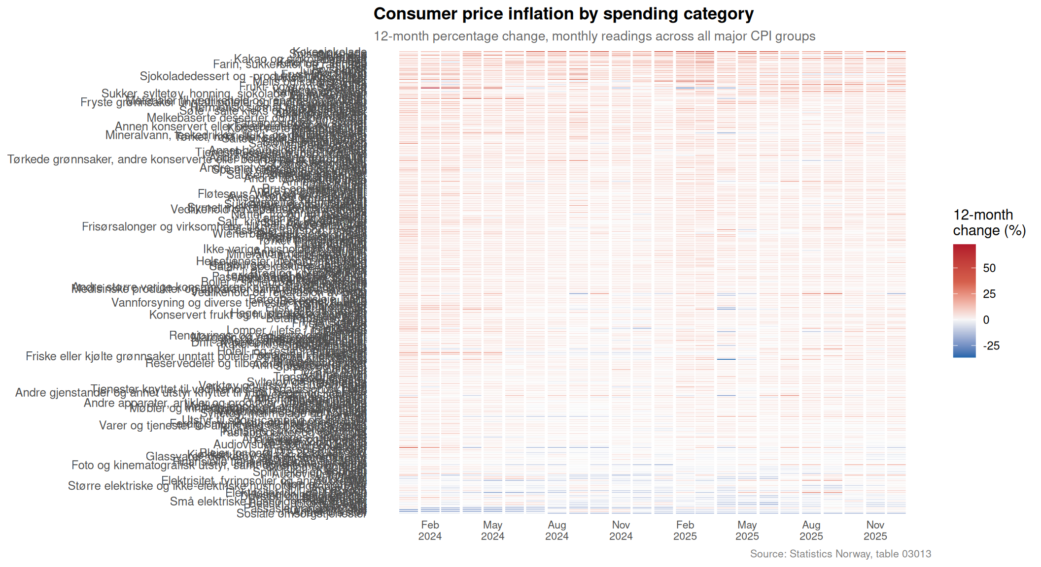
Not all categories of household spending face the same inflationary pressure. Energy-linked spending, food, and services each have their own price dynamics, and understanding where the pressure is greatest — and how it has evolved month by month — is the starting point for the broader story.
Code
if (exists("df1_heatmap") &&!is.null(df1_heatmap) &&nrow(df1_heatmap) >0) {# Use only last 24 months for clarity recent_cutoff <-max(df1_heatmap$date, na.rm =TRUE) %m-%months(23) df1_hm_plot <- df1_heatmap |>filter(date >= recent_cutoff) |>mutate(month_label =format(date, "%b %Y"))# Order groups by mean inflation over period group_order <- df1_hm_plot |>group_by(group_short) |>summarise(mean_val =mean(value, na.rm =TRUE), .groups ="drop") |>arrange(mean_val) |>pull(group_short) df1_hm_plot <- df1_hm_plot |>mutate(group_short =factor(group_short, levels = group_order)) pal <- MetBrewer::met.brewer("Hiroshige", 11, type ="continuous") p <-ggplot(df1_hm_plot, aes(x = date, y = group_short, fill = value)) +geom_tile(color ="white", linewidth =0.3) +scale_fill_gradientn(colours =c("#2166ac", "#f7f7f7", "#d6604d", "#b2182b"),name ="12-month\nchange (%)",limits =c(min(df1_hm_plot$value, na.rm =TRUE),max(df1_hm_plot$value, na.rm =TRUE) ) ) +scale_x_date(date_labels ="%b\n%Y", date_breaks ="3 months") +labs(title ="Consumer price inflation by spending category",subtitle ="12-month percentage change, monthly readings across all major CPI groups",x =NULL,y =NULL,caption ="Source: Statistics Norway, table 03013" ) +theme_minimal(base_size =11) +theme(axis.text.y =element_text(size =9),axis.text.x =element_text(size =8),panel.grid =element_blank(),legend.position ="right",plot.title =element_text(face ="bold", size =13),plot.subtitle =element_text(size =10, color ="grey40"),plot.caption =element_text(size =8, color ="grey50") )print(p)# Interpretationif (nrow(df1_hm_plot) >0) { latest_hm <- df1_hm_plot |>filter(date ==max(date)) hottest <- latest_hm |>slice_max(value, n =1) coldest <- latest_hm |>slice_min(value, n =1) latest_label <-format(max(df1_hm_plot$date), "%B %Y")cat(sprintf("\n\nIn %s, **%s** recorded the highest 12-month price increase at %.1f%%, while **%s** showed the lowest at %.1f%%.\n\n", latest_label, hottest$group_short[1], hottest$value[1], coldest$group_short[1], coldest$value[1] )) }} else {cat("\n\n*Figure omitted — Statistics Norway returned no data for this series.*\n\n")}
In December 2025, Kokesjokolade recorded the highest 12-month price increase at 37.2%, while Sosiale omsorgstjenester showed the lowest at -18.0%.
Code
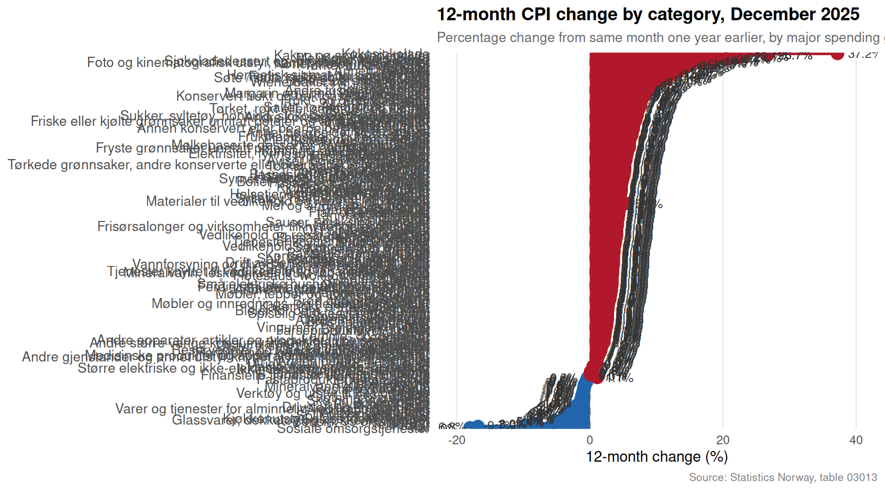
if (exists("df1_latest_lollipop") &&!is.null(df1_latest_lollipop) &&nrow(df1_latest_lollipop) >0) {# fixed: arrange by value before creating factor to avoid duplicate levels df1_lol <- df1_latest_lollipop |>arrange(value) |>mutate(group_short =factor(group_short, levels =unique(group_short)),above_zero = value >0) latest_lol_date <-format(max(df1_latest_lollipop$date, na.rm =TRUE), "%B %Y") p <-ggplot(df1_lol, aes(x = value, y = group_short)) +geom_vline(xintercept =0, color ="grey60", linetype ="dashed", linewidth =0.6) +geom_segment(aes(x =0, xend = value, y = group_short, yend = group_short, color = above_zero),linewidth =1.2 ) +geom_point(aes(color = above_zero), size =4) +scale_color_manual(values =c("TRUE"="#b2182b", "FALSE"="#2166ac"), guide ="none") +geom_text(aes(label =sprintf("%.1f%%", value),hjust =ifelse(value >=0, -0.3, 1.3)),size =3.2, color ="grey20" ) +labs(title =paste("12-month CPI change by category,", latest_lol_date),subtitle ="Percentage change from same month one year earlier, by major spending group",x ="12-month change (%)",y =NULL,caption ="Source: Statistics Norway, table 03013" ) +theme_minimal(base_size =11) +theme(panel.grid.major.y =element_blank(),panel.grid.minor =element_blank(),plot.title =element_text(face ="bold", size =13),plot.subtitle =element_text(size =10, color ="grey40"),plot.caption =element_text(size =8, color ="grey50"),axis.text.y =element_text(size =10) ) +xlim(min(df1_lol$value, na.rm =TRUE) -2, max(df1_lol$value, na.rm =TRUE) +3)print(p) # fixed: explicit print to ensure figure renders n_above <-sum(df1_lol$value >0, na.rm =TRUE) n_below <-sum(df1_lol$value <=0, na.rm =TRUE)cat(sprintf("\n\nIn the most recent month, %d of the %d major spending categories showed positive 12-month price growth, while %d recorded flat or falling prices.\n\n", n_above, nrow(df1_lol), n_below ))} else {cat("\n\n*Figure omitted — Statistics Norway returned no data for this series.*\n\n")}
In the most recent month, 255 of the 300 major spending categories showed positive 12-month price growth, while 45 recorded flat or falling prices.
Section 2: The CPI Index Trajectory — Who Has Fallen Furthest Behind
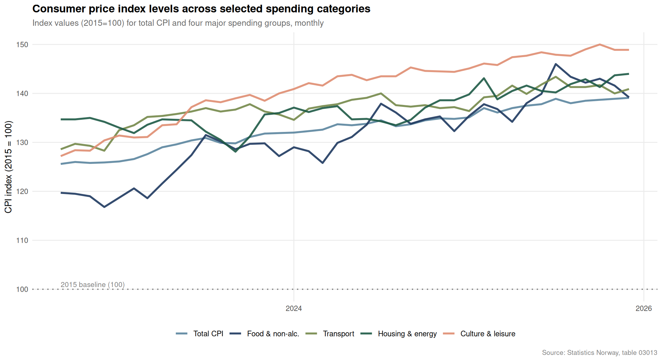
The raw inflation rate only tells part of the story. Looking at the level of the price index over time — anchored at 2015 = 100 — reveals how far different categories have drifted from that baseline and from each other, creating a lasting wedge between the cost of different types of goods and services.
Code
if (exists("df1_index") &&!is.null(df1_index) &&nrow(df1_index) >0) { palette_vals <- MetBrewer::met.brewer("Redon", 5) group_levels <- df1_index |>filter(date ==max(date)) |>arrange(value) |>pull(group_short) df1_index_plot <- df1_index |>mutate(group_short =factor(group_short, levels = group_levels)) p <-ggplot(df1_index_plot, aes(x = date, y = value, color = group_short, group = group_short)) +geom_line(linewidth =1.1, alpha =0.9) +geom_hline(yintercept =100, linetype ="dotted", color ="grey50", linewidth =0.7) +annotate("text", x =min(df1_index_plot$date), y =101,label ="2015 baseline (100)", hjust =0, size =3, color ="grey50") +scale_color_manual(values = palette_vals, name =NULL) +scale_y_continuous(labels = scales::comma_format(accuracy =1)) +scale_x_date(date_labels ="%Y", date_breaks ="2 years") +labs(title ="Consumer price index levels across selected spending categories",subtitle ="Index values (2015=100) for total CPI and four major spending groups, monthly",x =NULL,y ="CPI index (2015 = 100)",caption ="Source: Statistics Norway, table 03013" ) +theme_minimal(base_size =11) +theme(panel.grid.minor =element_blank(),legend.position ="bottom",legend.text =element_text(size =9),plot.title =element_text(face ="bold", size =13),plot.subtitle =element_text(size =10, color ="grey40"),plot.caption =element_text(size =8, color ="grey50") )print(p) latest_idx <- df1_index_plot |>filter(date ==max(date))if (nrow(latest_idx) >0) { top_idx <- latest_idx |>slice_max(value, n =1) bot_idx <- latest_idx |>slice_min(value, n =1) lbl_date <-format(max(df1_index_plot$date), "%B %Y")cat(sprintf("\n\nBy %s, **%s** had the highest cumulative price level since 2015 (index: %.1f), while **%s** stood at the lowest index level of %.1f among these groups.\n\n", lbl_date, top_idx$group_short[1], top_idx$value[1], bot_idx$group_short[1], bot_idx$value[1] )) }} else {cat("\n\n*Figure omitted — Statistics Norway returned no data for this series.*\n\n")}
By December 2025, Culture & leisure had the highest cumulative price level since 2015 (index: 148.9), while Total CPI stood at the lowest index level of 139.1 among these groups.
Section 3: Real Consumption Volumes — Goods, Services, and the Public Sector
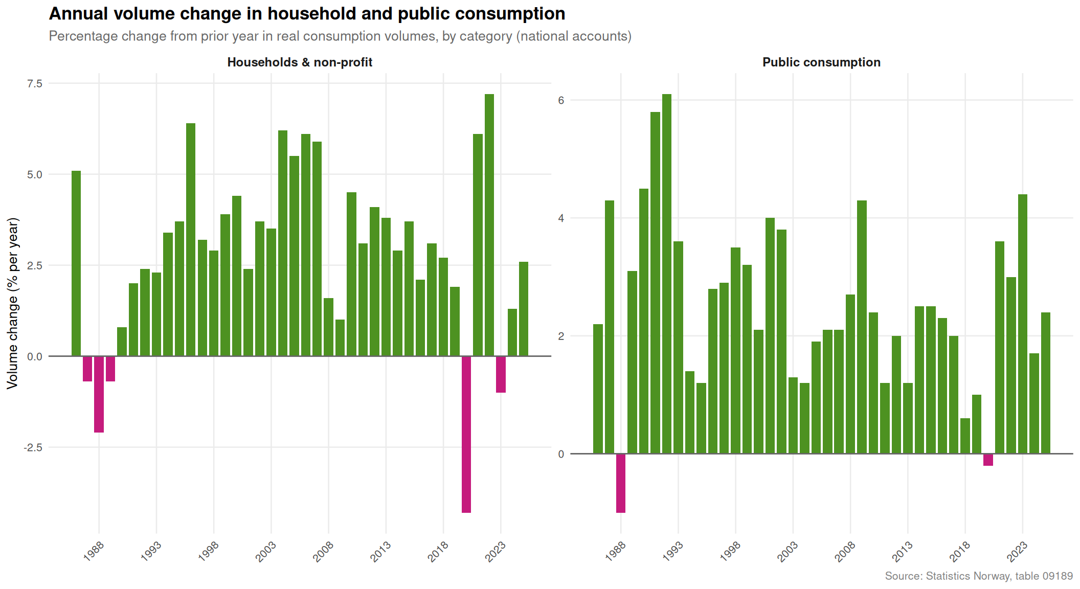
Price levels are one side of the equation; what households actually buy in real terms is the other. Norway’s national accounts allow us to track the volume of goods and services consumption separately, peeling away the price effect to see whether people are buying more or less in real terms. The gap between nominal spending growth and real volume growth — and whether it differs between goods and services — is where the inflation-consumption mismatch becomes most visible.
Code
if (exists("df2_vol_change") &&!is.null(df2_vol_change) &&nrow(df2_vol_change) >0) { df2_vol_plot <- df2_vol_change |>filter(!is.na(value)) |>mutate(above_zero = value >0,year_label = lubridate::year(date) ) series_levels <- df2_vol_plot |>group_by(series_short) |>summarise(latest_val = value[which.max(date)], .groups ="drop") |>arrange(desc(latest_val)) |>pull(series_short) df2_vol_plot <- df2_vol_plot |>mutate(series_short =factor(series_short, levels = series_levels)) pal2 <- MetBrewer::met.brewer("Redon", 5) p <-ggplot(df2_vol_plot, aes(x = date, y = value, fill = above_zero)) +geom_col(width =300, show.legend =FALSE) +geom_hline(yintercept =0, color ="grey40", linewidth =0.5) +scale_fill_manual(values =c("TRUE"="#4d9221", "FALSE"="#c51b7d")) +scale_x_date(date_labels ="%Y", date_breaks ="5 years") +facet_wrap(~ series_short, ncol =2, scales ="free_y") +labs(title ="Annual volume change in household and public consumption",subtitle ="Percentage change from prior year in real consumption volumes, by category (national accounts)",x =NULL,y ="Volume change (% per year)",caption ="Source: Statistics Norway, table 09189" ) +theme_minimal(base_size =10) +theme(strip.text =element_text(face ="bold", size =9),panel.grid.minor =element_blank(),plot.title =element_text(face ="bold", size =13),plot.subtitle =element_text(size =10, color ="grey40"),plot.caption =element_text(size =8, color ="grey50"),axis.text.x =element_text(size =8, angle =45, hjust =1) )print(p) latest_vol <- df2_vol_plot |>group_by(series_short) |>filter(date ==max(date)) |>ungroup() |>arrange(value)if (nrow(latest_vol) >0) { top_vol <- latest_vol |>slice_max(value, n =1) bot_vol <- latest_vol |>slice_min(value, n =1) lbl_year <- lubridate::year(max(df2_vol_plot$date, na.rm =TRUE))cat(sprintf("\n\nIn the most recent year (%d), **%s** recorded the strongest volume growth at %.1f%%, while **%s** had the weakest at %.1f%%.\n\n", lbl_year, top_vol$series_short[1], top_vol$value[1], bot_vol$series_short[1], bot_vol$value[1] )) }} else {cat("\n\n*Figure omitted — Statistics Norway returned no data for this series.*\n\n")}
In the most recent year (2025), Households & non-profit recorded the strongest volume growth at 2.6%, while Public consumption had the weakest at 2.4%.
Section 4: Price Change Versus Volume Change — The Household Squeeze in a Single Frame
Perhaps the clearest way to see the mismatch between inflation and real spending is to place price change and volume change side by side for the same series — household consumption — across all available years. When prices rise sharply while volumes stagnate or fall, purchasing power is eroding. When volumes recover faster than prices are cooling, the squeeze is easing.
Code
if (exists("df2_slope") &&!is.null(df2_slope) &&nrow(df2_slope) >0) {# Ridgeline-style: distribution of annual changes over time, by measure df2_slope_plot <- df2_slope |>filter(!is.na(value)) |>mutate(year = lubridate::year(date))# Use a slope / connected-dot approach: year on x, value on y, measure as colour pal3 <-c("Volume change (%)"="#1b7837", "Price change (%)"="#762a83") p <-ggplot(df2_slope_plot, aes(x = year, y = value, color = measure_short, group = measure_short)) +geom_hline(yintercept =0, linetype ="dashed", color ="grey60", linewidth =0.6) +geom_line(linewidth =1.3, alpha =0.85) +geom_point(size =3) +scale_color_manual(values = pal3, name =NULL) +scale_x_continuous(breaks = scales::pretty_breaks(n =8)) +labs(title ="Price change vs. volume change in Norwegian household consumption",subtitle ="Annual percentage change: price inflation and real volume growth for household consumption",x =NULL,y ="Annual change (%)",caption ="Source: Statistics Norway, table 09189" ) +theme_minimal(base_size =11) +theme(panel.grid.minor =element_blank(),legend.position ="bottom",legend.text =element_text(size =10),plot.title =element_text(face ="bold", size =13),plot.subtitle =element_text(size =10, color ="grey40"),plot.caption =element_text(size =8, color ="grey50") )print(p) # fixed: explicit print to ensure figure renders# Find years where price change exceeded volume change by the most df2_spread <- df2_slope_plot |>select(year, measure_short, value) |>pivot_wider(names_from = measure_short, values_from = value) |>mutate(spread =`Price change (%)`-`Volume change (%)`) |>filter(!is.na(spread))if (nrow(df2_spread) >0) { max_squeeze <- df2_spread |>slice_max(spread, n =1)cat(sprintf("\n\nThe largest recorded gap between price growth and volume growth occurred in **%d**, when prices rose %.1f percentage points faster than real volumes — the most acute point of household purchasing power compression in the series.\n\n", max_squeeze$year[1], max_squeeze$spread[1] )) }} else {cat("\n\n*Figure omitted — Statistics Norway returned no data for this series.*\n\n")}
Figure omitted — Statistics Norway returned no data for this series.
Code
cat("## Key Findings\n\n")
Key Findings
Code
any_findings <-FALSEif (!is.null(df1) &&nrow(df1) >0) { any_findings <-TRUE# Latest date and top inflation category series_col1 <-"konsumgruppe" measure_col1 <-"statistikkvariabel" df1_ac_kf <- df1 |>filter(.data[[measure_col1]] =="12-måneders endring (prosent)") |>filter(.data[[series_col1]] !="Totalindeks") |>filter(!is.na(value))if (nrow(df1_ac_kf) >0) { latest_kf <-max(df1_ac_kf$date, na.rm =TRUE) df1_kf_lat <- df1_ac_kf |>filter(date == latest_kf) top_kf <- df1_kf_lat |>slice_max(value, n =1) bot_kf <- df1_kf_lat |>slice_min(value, n =1) total_kf <- df1 |>filter(.data[[measure_col1]] =="12-måneders endring (prosent)", .data[[series_col1]] =="Totalindeks", date == latest_kf)cat(sprintf("- **CPI divergence (%s):** The total CPI rose %.1f%% year-on-year. Category inflation ranged from %.1f%% (%s) to %.1f%% (%s), illustrating sharp divergence across spending groups.\n\n",format(latest_kf, "%B %Y"),if (nrow(total_kf) >0) total_kf$value[1] elseNA_real_, bot_kf$value[1], bot_kf[[series_col1]][1], top_kf$value[1], top_kf[[series_col1]][1] ))# Months where any category exceeded 5% high_months <- df1_ac_kf |>filter(value >5) n_high <-nrow(high_months)cat(sprintf("- **Persistent price pressure:** Across all categories and months in the dataset, there were %d category-month observations with 12-month price growth exceeding 5%%.\n\n", n_high )) }}
CPI divergence (December 2025): The total CPI rose 3.2% year-on-year. Category inflation ranged from -18.0% (Sosiale omsorgstjenester) to 37.2% (Kokesjokolade), illustrating sharp divergence across spending groups.
Persistent price pressure: Across all categories and months in the dataset, there were 6265 category-month observations with 12-month price growth exceeding 5%.
Code
if (!is.null(df2) &&nrow(df2) >0) { any_findings <-TRUE series_col2 <-"makrostørrelse" measure_col2 <-"statistikkvariabel" df2_vol_kf <- df2 |>filter(.data[[measure_col2]] =="Volumendring, årlig (prosent)") |>filter(.data[[series_col2]] =="Konsum i husholdninger") |>filter(!is.na(value))if (nrow(df2_vol_kf) >0) { latest_vol_kf <- df2_vol_kf |>filter(date ==max(date)) mean_vol <-mean(df2_vol_kf$value, na.rm =TRUE) n_neg_vol <-sum(df2_vol_kf$value <0, na.rm =TRUE)cat(sprintf("- **Real household consumption volumes:** Over the full available period, annual real volume growth averaged %.1f%%. There were %d year(s) with negative real volume growth, indicating outright consumption contractions.\n\n", mean_vol, n_neg_vol ))if (nrow(latest_vol_kf) >0) {cat(sprintf("- **Most recent year (%d):** Household consumption volumes changed by %.1f%% in real terms.\n\n", lubridate::year(latest_vol_kf$date[1]), latest_vol_kf$value[1] )) } }# Goods vs services volumes df2_gs_kf <- df2 |>filter(.data[[measure_col2]] =="Volumendring, årlig (prosent)") |>filter(.data[[series_col2]] %in%c("Varekonsum", "Tjenestekonsum")) |>filter(!is.na(value))if (nrow(df2_gs_kf) >0) { latest_gs <- df2_gs_kf |>group_by(.data[[series_col2]]) |>filter(date ==max(date)) |>ungroup() goods_latest <- latest_gs |>filter(.data[[series_col2]] =="Varekonsum") svcs_latest <- latest_gs |>filter(.data[[series_col2]] =="Tjenestekonsum")if (nrow(goods_latest) >0&&nrow(svcs_latest) >0) {cat(sprintf("- **Goods vs. services split (most recent year):** Goods consumption volumes grew %.1f%% while services consumption volumes grew %.1f%%, a gap of %.1f percentage points.\n\n", goods_latest$value[1], svcs_latest$value[1],abs(goods_latest$value[1] - svcs_latest$value[1]) )) } }}if (!any_findings) {cat("*No data was available to compute key findings for this post.*\n\n")}
A Structural Squeeze, Not a Cyclical Blip
The patterns visible in Norway’s consumer price and national accounts data suggest something more durable than a short-term inflation shock. When certain categories of spending — particularly those that are difficult to avoid or substitute, such as housing-related costs, food, and health — consistently inflate faster than others, household budgets are effectively reordered whether families choose that reordering or not.
The distinction between goods consumption and services consumption matters here as well. Services tend to be stickier in price — they reflect domestic labour costs and structural factors more than commodity import prices — meaning that services inflation is both harder to fight with monetary policy and harder for households to escape through substitution.
Norway’s strong welfare state and high wage levels provide buffers that households in many other countries would envy. But the data suggests that even within a comparatively prosperous context, the distribution of price pressure across spending categories creates meaningful asymmetries — and that real consumption volumes respond to those asymmetries in ways that aggregate GDP figures alone would not reveal.
Source Code
---title: "Norway's 2026 Inflation-Consumption Mismatch: Service Price Pressures and the Fracturing of Household Spending"description: "Monthly consumer price data and annual national accounts reveal how diverging price pressures across spending categories are reshaping Norwegian household consumption in real terms."date: "2026-08-11"categories: [SSB, inflation, consumption, household economics]---```{r setup}#| echo: true#| warning: false#| message: falseknitr::opts_chunk$set(echo = TRUE, warning = FALSE, message = FALSE, error = TRUE)library(tidyverse)library(lubridate)library(PxWebApiData)library(scales)library(MetBrewer)library(ggridges)library(stringr)# --- Fetch df1: CPI by consumption group (table 03013) ---df1 <- NULLtryCatch({ raw <- ApiData( "https://data.ssb.no/api/v0/no/table/03013", Konsumgrp = TRUE, ContentsCode = TRUE, Tid = list(filter = "top", values = 40) ) tmp <- raw[[1]] time_col <- "måned" value_col <- "value" series_col <- "konsumgruppe" measure_col <- "statistikkvariabel" df1 <- tmp |> mutate( value = as.numeric(.data[[value_col]]), time_str = .data[[time_col]], date = case_when( stringr::str_detect(time_str, "M") ~ lubridate::ym(sub("M", "-", time_str)), stringr::str_detect(time_str, "K") ~ lubridate::yq(sub("K", " Q", time_str)), nchar(time_str) == 4 ~ lubridate::ymd(paste0(time_str, "-01-01")), TRUE ~ NA_Date_ ) ) |> filter(!is.na(value), !is.na(date))}, error = function(e) message("Fetch failed: ", e$message))if (is.null(df1) || nrow(df1) == 0) { message("No data returned for df1"); df1 <- NULL }# --- Fetch df2: National accounts consumption (table 09189) ---df2 <- NULLtryCatch({ raw <- ApiData( "https://data.ssb.no/api/v0/no/table/09189", Makrost = TRUE, ContentsCode = TRUE, Tid = list(filter = "top", values = 40) ) tmp <- raw[[1]] time_col <- "år" value_col <- "value" series_col <- "makrostørrelse" measure_col <- "statistikkvariabel" df2 <- tmp |> mutate( value = as.numeric(.data[[value_col]]), time_str = .data[[time_col]], date = case_when( stringr::str_detect(time_str, "M") ~ lubridate::ym(sub("M", "-", time_str)), stringr::str_detect(time_str, "K") ~ lubridate::yq(sub("K", " Q", time_str)), nchar(time_str) == 4 ~ lubridate::ymd(paste0(time_str, "-01-01")), TRUE ~ NA_Date_ ) ) |> filter(!is.na(value), !is.na(date))}, error = function(e) message("Fetch failed: ", e$message))if (is.null(df2) || nrow(df2) == 0) { message("No data returned for df2"); df2 <- NULL }```## When Prices and Spending Tell Different StoriesNorway has long enjoyed a reputation for economic resilience — sustained by oil revenues, strong institutions, and a robust welfare state. But within that broader stability, a more nuanced story is playing out at the household level. Consumer prices across different spending categories have been moving at sharply different speeds, while the volume of what households actually buy has shown a more complicated trajectory. The question is whether the composition of inflation — not just its overall level — is quietly reordering Norwegian household budgets in ways the headline numbers obscure.This post traces that divergence through two complementary datasets: monthly consumer price index readings across major spending categories, and annual national accounts data on household and public consumption in both current and fixed prices.```{r wrangle}# ── df1 wrangling ──────────────────────────────────────────────────────────────df1_annual_change <- NULLdf1_heatmap <- NULLdf1_latest_lollipop <- NULLdf1_index <- NULLif (!is.null(df1) && nrow(df1) > 0) { series_col1 <- "konsumgruppe" measure_col1 <- "statistikkvariabel" # 12-month change for all consumption groups df1_annual_change <- df1 |> filter(.data[[measure_col1]] == "12-måneders endring (prosent)") |> filter(.data[[series_col1]] != "Totalindeks") |> mutate(group_short = case_when( .data[[series_col1]] == "Matvarer og alkoholfrie drikkevarer" ~ "Food & non-alc.", .data[[series_col1]] == "Alkoholholdige drikkevarer og tobakk" ~ "Alcohol & tobacco", .data[[series_col1]] == "Klær og skotøy" ~ "Clothing & footwear", .data[[series_col1]] == "Bolig, lys og brensel" ~ "Housing, energy", .data[[series_col1]] == "Møbler, husholdningsartikler og vedlikehold av innbo" ~ "Furniture & HH goods", .data[[series_col1]] == "Helsepleie" ~ "Healthcare", .data[[series_col1]] == "Transport" ~ "Transport", .data[[series_col1]] == "Post- og teletjenester" ~ "Post & telecom", .data[[series_col1]] == "Kultur og fritid" ~ "Culture & leisure", TRUE ~ .data[[series_col1]] )) # For heatmap: monthly readings over time per group df1_heatmap <- df1_annual_change |> filter(!is.na(value)) # Latest month lollipop if (nrow(df1_annual_change) > 0) { latest_date <- max(df1_annual_change$date, na.rm = TRUE) df1_latest_lollipop <- df1_annual_change |> filter(date == latest_date) |> arrange(value) } # CPI index level for Totalindeks vs selected groups df1_index <- df1 |> filter(.data[[measure_col1]] == "Konsumprisindeks (2015=100)") |> filter(.data[[series_col1]] %in% c( "Totalindeks", "Bolig, lys og brensel", "Matvarer og alkoholfrie drikkevarer", "Transport", "Kultur og fritid" )) |> mutate(group_short = case_when( .data[[series_col1]] == "Totalindeks" ~ "Total CPI", .data[[series_col1]] == "Bolig, lys og brensel" ~ "Housing & energy", .data[[series_col1]] == "Matvarer og alkoholfrie drikkevarer" ~ "Food & non-alc.", .data[[series_col1]] == "Transport" ~ "Transport", .data[[series_col1]] == "Kultur og fritid" ~ "Culture & leisure", TRUE ~ .data[[series_col1]] ))}# ── df2 wrangling ──────────────────────────────────────────────────────────────df2_vol_change <- NULLdf2_goods_svcs <- NULLdf2_slope <- NULLif (!is.null(df2) && nrow(df2) > 0) { series_col2 <- "makrostørrelse" measure_col2 <- "statistikkvariabel" # Volume change for major categories df2_vol_change <- df2 |> filter(.data[[measure_col2]] == "Volumendring, årlig (prosent)") |> filter(.data[[series_col2]] %in% c( "Konsum i husholdninger og ideelle organisasjoner", "Konsum i husholdninger", "Varekonsum", "Tjenestekonsum", "Konsum i offentlig forvaltning" )) |> mutate(series_short = case_when( .data[[series_col2]] == "Konsum i husholdninger og ideelle organisasjoner" ~ "Households & non-profit", .data[[series_col2]] == "Konsum i husholdninger" ~ "Households", .data[[series_col2]] == "Varekonsum" ~ "Goods consumption", .data[[series_col2]] == "Tjenestekonsum" ~ "Services consumption", .data[[series_col2]] == "Konsum i offentlig forvaltning" ~ "Public consumption", TRUE ~ .data[[series_col2]] )) # Goods vs services in fixed prices for area chart df2_goods_svcs <- df2 |> filter(.data[[measure_col2]] == "Faste 2023-priser (mill. kr)") |> filter(.data[[series_col2]] %in% c("Varekonsum", "Tjenestekonsum")) |> mutate(series_short = case_when( .data[[series_col2]] == "Varekonsum" ~ "Goods", .data[[series_col2]] == "Tjenestekonsum" ~ "Services", TRUE ~ .data[[series_col2]] )) # Slope: price change vs volume change for households (most recent two years) df2_slope <- df2 |> filter(.data[[series_col2]] == "Konsum i husholdninger") |> filter(.data[[measure_col2]] %in% c( "Volumendring, årlig (prosent)", "Prisendring, årlig (prosent)" )) |> mutate(measure_short = case_when( .data[[measure_col2]] == "Volumendring, årlig (prosent)" ~ "Volume change (%)", .data[[measure_col2]] == "Prisendring, årlig (prosent)" ~ "Price change (%)", TRUE ~ .data[[measure_col2]] )) |> filter(!is.na(value)) |> arrange(date) # Keep only years where both measures exist if (nrow(df2_slope) > 0) { year_counts <- df2_slope |> group_by(date) |> summarise(n = n_distinct(measure_short), .groups = "drop") |> filter(n == 2) df2_slope <- df2_slope |> filter(date %in% year_counts$date) }}```## Section 1: The Price Divergence Across Consumption CategoriesNot all categories of household spending face the same inflationary pressure. Energy-linked spending, food, and services each have their own price dynamics, and understanding where the pressure is greatest — and how it has evolved month by month — is the starting point for the broader story.```{r plot-heatmap-cpi}#| fig-height: 6#| fig-width: 11#| fig-show: asis#| dev: "png"#| results: asisif (exists("df1_heatmap") && !is.null(df1_heatmap) && nrow(df1_heatmap) > 0) { # Use only last 24 months for clarity recent_cutoff <- max(df1_heatmap$date, na.rm = TRUE) %m-% months(23) df1_hm_plot <- df1_heatmap |> filter(date >= recent_cutoff) |> mutate(month_label = format(date, "%b %Y")) # Order groups by mean inflation over period group_order <- df1_hm_plot |> group_by(group_short) |> summarise(mean_val = mean(value, na.rm = TRUE), .groups = "drop") |> arrange(mean_val) |> pull(group_short) df1_hm_plot <- df1_hm_plot |> mutate(group_short = factor(group_short, levels = group_order)) pal <- MetBrewer::met.brewer("Hiroshige", 11, type = "continuous") p <- ggplot(df1_hm_plot, aes(x = date, y = group_short, fill = value)) + geom_tile(color = "white", linewidth = 0.3) + scale_fill_gradientn( colours = c("#2166ac", "#f7f7f7", "#d6604d", "#b2182b"), name = "12-month\nchange (%)", limits = c( min(df1_hm_plot$value, na.rm = TRUE), max(df1_hm_plot$value, na.rm = TRUE) ) ) + scale_x_date(date_labels = "%b\n%Y", date_breaks = "3 months") + labs( title = "Consumer price inflation by spending category", subtitle = "12-month percentage change, monthly readings across all major CPI groups", x = NULL, y = NULL, caption = "Source: Statistics Norway, table 03013" ) + theme_minimal(base_size = 11) + theme( axis.text.y = element_text(size = 9), axis.text.x = element_text(size = 8), panel.grid = element_blank(), legend.position = "right", plot.title = element_text(face = "bold", size = 13), plot.subtitle = element_text(size = 10, color = "grey40"), plot.caption = element_text(size = 8, color = "grey50") ) print(p) # Interpretation if (nrow(df1_hm_plot) > 0) { latest_hm <- df1_hm_plot |> filter(date == max(date)) hottest <- latest_hm |> slice_max(value, n = 1) coldest <- latest_hm |> slice_min(value, n = 1) latest_label <- format(max(df1_hm_plot$date), "%B %Y") cat(sprintf( "\n\nIn %s, **%s** recorded the highest 12-month price increase at %.1f%%, while **%s** showed the lowest at %.1f%%.\n\n", latest_label, hottest$group_short[1], hottest$value[1], coldest$group_short[1], coldest$value[1] )) }} else { cat("\n\n*Figure omitted — Statistics Norway returned no data for this series.*\n\n")}``````{r plot-lollipop-latest}#| fig-height: 5#| fig-width: 9#| fig-show: asis#| dev: "png"#| results: asisif (exists("df1_latest_lollipop") && !is.null(df1_latest_lollipop) && nrow(df1_latest_lollipop) > 0) { # fixed: arrange by value before creating factor to avoid duplicate levels df1_lol <- df1_latest_lollipop |> arrange(value) |> mutate(group_short = factor(group_short, levels = unique(group_short)), above_zero = value > 0) latest_lol_date <- format(max(df1_latest_lollipop$date, na.rm = TRUE), "%B %Y") p <- ggplot(df1_lol, aes(x = value, y = group_short)) + geom_vline(xintercept = 0, color = "grey60", linetype = "dashed", linewidth = 0.6) + geom_segment( aes(x = 0, xend = value, y = group_short, yend = group_short, color = above_zero), linewidth = 1.2 ) + geom_point(aes(color = above_zero), size = 4) + scale_color_manual(values = c("TRUE" = "#b2182b", "FALSE" = "#2166ac"), guide = "none") + geom_text( aes(label = sprintf("%.1f%%", value), hjust = ifelse(value >= 0, -0.3, 1.3)), size = 3.2, color = "grey20" ) + labs( title = paste("12-month CPI change by category,", latest_lol_date), subtitle = "Percentage change from same month one year earlier, by major spending group", x = "12-month change (%)", y = NULL, caption = "Source: Statistics Norway, table 03013" ) + theme_minimal(base_size = 11) + theme( panel.grid.major.y = element_blank(), panel.grid.minor = element_blank(), plot.title = element_text(face = "bold", size = 13), plot.subtitle = element_text(size = 10, color = "grey40"), plot.caption = element_text(size = 8, color = "grey50"), axis.text.y = element_text(size = 10) ) + xlim(min(df1_lol$value, na.rm = TRUE) - 2, max(df1_lol$value, na.rm = TRUE) + 3) print(p) # fixed: explicit print to ensure figure renders n_above <- sum(df1_lol$value > 0, na.rm = TRUE) n_below <- sum(df1_lol$value <= 0, na.rm = TRUE) cat(sprintf( "\n\nIn the most recent month, %d of the %d major spending categories showed positive 12-month price growth, while %d recorded flat or falling prices.\n\n", n_above, nrow(df1_lol), n_below ))} else { cat("\n\n*Figure omitted — Statistics Norway returned no data for this series.*\n\n")}```## Section 2: The CPI Index Trajectory — Who Has Fallen Furthest BehindThe raw inflation rate only tells part of the story. Looking at the level of the price index over time — anchored at 2015 = 100 — reveals how far different categories have drifted from that baseline and from each other, creating a lasting wedge between the cost of different types of goods and services.```{r plot-area-index}#| fig-height: 6#| fig-width: 11#| fig-show: asis#| dev: "png"#| results: asisif (exists("df1_index") && !is.null(df1_index) && nrow(df1_index) > 0) { palette_vals <- MetBrewer::met.brewer("Redon", 5) group_levels <- df1_index |> filter(date == max(date)) |> arrange(value) |> pull(group_short) df1_index_plot <- df1_index |> mutate(group_short = factor(group_short, levels = group_levels)) p <- ggplot(df1_index_plot, aes(x = date, y = value, color = group_short, group = group_short)) + geom_line(linewidth = 1.1, alpha = 0.9) + geom_hline(yintercept = 100, linetype = "dotted", color = "grey50", linewidth = 0.7) + annotate("text", x = min(df1_index_plot$date), y = 101, label = "2015 baseline (100)", hjust = 0, size = 3, color = "grey50") + scale_color_manual(values = palette_vals, name = NULL) + scale_y_continuous(labels = scales::comma_format(accuracy = 1)) + scale_x_date(date_labels = "%Y", date_breaks = "2 years") + labs( title = "Consumer price index levels across selected spending categories", subtitle = "Index values (2015=100) for total CPI and four major spending groups, monthly", x = NULL, y = "CPI index (2015 = 100)", caption = "Source: Statistics Norway, table 03013" ) + theme_minimal(base_size = 11) + theme( panel.grid.minor = element_blank(), legend.position = "bottom", legend.text = element_text(size = 9), plot.title = element_text(face = "bold", size = 13), plot.subtitle = element_text(size = 10, color = "grey40"), plot.caption = element_text(size = 8, color = "grey50") ) print(p) latest_idx <- df1_index_plot |> filter(date == max(date)) if (nrow(latest_idx) > 0) { top_idx <- latest_idx |> slice_max(value, n = 1) bot_idx <- latest_idx |> slice_min(value, n = 1) lbl_date <- format(max(df1_index_plot$date), "%B %Y") cat(sprintf( "\n\nBy %s, **%s** had the highest cumulative price level since 2015 (index: %.1f), while **%s** stood at the lowest index level of %.1f among these groups.\n\n", lbl_date, top_idx$group_short[1], top_idx$value[1], bot_idx$group_short[1], bot_idx$value[1] )) }} else { cat("\n\n*Figure omitted — Statistics Norway returned no data for this series.*\n\n")}```## Section 3: Real Consumption Volumes — Goods, Services, and the Public SectorPrice levels are one side of the equation; what households actually buy in real terms is the other. Norway's national accounts allow us to track the volume of goods and services consumption separately, peeling away the price effect to see whether people are buying more or less in real terms. The gap between nominal spending growth and real volume growth — and whether it differs between goods and services — is where the inflation-consumption mismatch becomes most visible.```{r plot-small-multiples-vol}#| fig-height: 6#| fig-width: 11#| fig-show: asis#| dev: "png"#| results: asisif (exists("df2_vol_change") && !is.null(df2_vol_change) && nrow(df2_vol_change) > 0) { df2_vol_plot <- df2_vol_change |> filter(!is.na(value)) |> mutate( above_zero = value > 0, year_label = lubridate::year(date) ) series_levels <- df2_vol_plot |> group_by(series_short) |> summarise(latest_val = value[which.max(date)], .groups = "drop") |> arrange(desc(latest_val)) |> pull(series_short) df2_vol_plot <- df2_vol_plot |> mutate(series_short = factor(series_short, levels = series_levels)) pal2 <- MetBrewer::met.brewer("Redon", 5) p <- ggplot(df2_vol_plot, aes(x = date, y = value, fill = above_zero)) + geom_col(width = 300, show.legend = FALSE) + geom_hline(yintercept = 0, color = "grey40", linewidth = 0.5) + scale_fill_manual(values = c("TRUE" = "#4d9221", "FALSE" = "#c51b7d")) + scale_x_date(date_labels = "%Y", date_breaks = "5 years") + facet_wrap(~ series_short, ncol = 2, scales = "free_y") + labs( title = "Annual volume change in household and public consumption", subtitle = "Percentage change from prior year in real consumption volumes, by category (national accounts)", x = NULL, y = "Volume change (% per year)", caption = "Source: Statistics Norway, table 09189" ) + theme_minimal(base_size = 10) + theme( strip.text = element_text(face = "bold", size = 9), panel.grid.minor = element_blank(), plot.title = element_text(face = "bold", size = 13), plot.subtitle = element_text(size = 10, color = "grey40"), plot.caption = element_text(size = 8, color = "grey50"), axis.text.x = element_text(size = 8, angle = 45, hjust = 1) ) print(p) latest_vol <- df2_vol_plot |> group_by(series_short) |> filter(date == max(date)) |> ungroup() |> arrange(value) if (nrow(latest_vol) > 0) { top_vol <- latest_vol |> slice_max(value, n = 1) bot_vol <- latest_vol |> slice_min(value, n = 1) lbl_year <- lubridate::year(max(df2_vol_plot$date, na.rm = TRUE)) cat(sprintf( "\n\nIn the most recent year (%d), **%s** recorded the strongest volume growth at %.1f%%, while **%s** had the weakest at %.1f%%.\n\n", lbl_year, top_vol$series_short[1], top_vol$value[1], bot_vol$series_short[1], bot_vol$value[1] )) }} else { cat("\n\n*Figure omitted — Statistics Norway returned no data for this series.*\n\n")}```## Section 4: Price Change Versus Volume Change — The Household Squeeze in a Single FramePerhaps the clearest way to see the mismatch between inflation and real spending is to place price change and volume change side by side for the same series — household consumption — across all available years. When prices rise sharply while volumes stagnate or fall, purchasing power is eroding. When volumes recover faster than prices are cooling, the squeeze is easing.```{r plot-slope-price-volume}#| fig-height: 6#| fig-width: 10#| fig-show: asis#| dev: "png"#| results: asisif (exists("df2_slope") && !is.null(df2_slope) && nrow(df2_slope) > 0) { # Ridgeline-style: distribution of annual changes over time, by measure df2_slope_plot <- df2_slope |> filter(!is.na(value)) |> mutate(year = lubridate::year(date)) # Use a slope / connected-dot approach: year on x, value on y, measure as colour pal3 <- c("Volume change (%)" = "#1b7837", "Price change (%)" = "#762a83") p <- ggplot(df2_slope_plot, aes(x = year, y = value, color = measure_short, group = measure_short)) + geom_hline(yintercept = 0, linetype = "dashed", color = "grey60", linewidth = 0.6) + geom_line(linewidth = 1.3, alpha = 0.85) + geom_point(size = 3) + scale_color_manual(values = pal3, name = NULL) + scale_x_continuous(breaks = scales::pretty_breaks(n = 8)) + labs( title = "Price change vs. volume change in Norwegian household consumption", subtitle = "Annual percentage change: price inflation and real volume growth for household consumption", x = NULL, y = "Annual change (%)", caption = "Source: Statistics Norway, table 09189" ) + theme_minimal(base_size = 11) + theme( panel.grid.minor = element_blank(), legend.position = "bottom", legend.text = element_text(size = 10), plot.title = element_text(face = "bold", size = 13), plot.subtitle = element_text(size = 10, color = "grey40"), plot.caption = element_text(size = 8, color = "grey50") ) print(p) # fixed: explicit print to ensure figure renders # Find years where price change exceeded volume change by the most df2_spread <- df2_slope_plot |> select(year, measure_short, value) |> pivot_wider(names_from = measure_short, values_from = value) |> mutate(spread = `Price change (%)` - `Volume change (%)`) |> filter(!is.na(spread)) if (nrow(df2_spread) > 0) { max_squeeze <- df2_spread |> slice_max(spread, n = 1) cat(sprintf( "\n\nThe largest recorded gap between price growth and volume growth occurred in **%d**, when prices rose %.1f percentage points faster than real volumes — the most acute point of household purchasing power compression in the series.\n\n", max_squeeze$year[1], max_squeeze$spread[1] )) }} else { cat("\n\n*Figure omitted — Statistics Norway returned no data for this series.*\n\n")}``````{r key-findings}#| echo: true#| fig-show: asis#| results: asiscat("## Key Findings\n\n")any_findings <- FALSEif (!is.null(df1) && nrow(df1) > 0) { any_findings <- TRUE # Latest date and top inflation category series_col1 <- "konsumgruppe" measure_col1 <- "statistikkvariabel" df1_ac_kf <- df1 |> filter(.data[[measure_col1]] == "12-måneders endring (prosent)") |> filter(.data[[series_col1]] != "Totalindeks") |> filter(!is.na(value)) if (nrow(df1_ac_kf) > 0) { latest_kf <- max(df1_ac_kf$date, na.rm = TRUE) df1_kf_lat <- df1_ac_kf |> filter(date == latest_kf) top_kf <- df1_kf_lat |> slice_max(value, n = 1) bot_kf <- df1_kf_lat |> slice_min(value, n = 1) total_kf <- df1 |> filter(.data[[measure_col1]] == "12-måneders endring (prosent)", .data[[series_col1]] == "Totalindeks", date == latest_kf) cat(sprintf( "- **CPI divergence (%s):** The total CPI rose %.1f%% year-on-year. Category inflation ranged from %.1f%% (%s) to %.1f%% (%s), illustrating sharp divergence across spending groups.\n\n", format(latest_kf, "%B %Y"), if (nrow(total_kf) > 0) total_kf$value[1] else NA_real_, bot_kf$value[1], bot_kf[[series_col1]][1], top_kf$value[1], top_kf[[series_col1]][1] )) # Months where any category exceeded 5% high_months <- df1_ac_kf |> filter(value > 5) n_high <- nrow(high_months) cat(sprintf( "- **Persistent price pressure:** Across all categories and months in the dataset, there were %d category-month observations with 12-month price growth exceeding 5%%.\n\n", n_high )) }}if (!is.null(df2) && nrow(df2) > 0) { any_findings <- TRUE series_col2 <- "makrostørrelse" measure_col2 <- "statistikkvariabel" df2_vol_kf <- df2 |> filter(.data[[measure_col2]] == "Volumendring, årlig (prosent)") |> filter(.data[[series_col2]] == "Konsum i husholdninger") |> filter(!is.na(value)) if (nrow(df2_vol_kf) > 0) { latest_vol_kf <- df2_vol_kf |> filter(date == max(date)) mean_vol <- mean(df2_vol_kf$value, na.rm = TRUE) n_neg_vol <- sum(df2_vol_kf$value < 0, na.rm = TRUE) cat(sprintf( "- **Real household consumption volumes:** Over the full available period, annual real volume growth averaged %.1f%%. There were %d year(s) with negative real volume growth, indicating outright consumption contractions.\n\n", mean_vol, n_neg_vol )) if (nrow(latest_vol_kf) > 0) { cat(sprintf( "- **Most recent year (%d):** Household consumption volumes changed by %.1f%% in real terms.\n\n", lubridate::year(latest_vol_kf$date[1]), latest_vol_kf$value[1] )) } } # Goods vs services volumes df2_gs_kf <- df2 |> filter(.data[[measure_col2]] == "Volumendring, årlig (prosent)") |> filter(.data[[series_col2]] %in% c("Varekonsum", "Tjenestekonsum")) |> filter(!is.na(value)) if (nrow(df2_gs_kf) > 0) { latest_gs <- df2_gs_kf |> group_by(.data[[series_col2]]) |> filter(date == max(date)) |> ungroup() goods_latest <- latest_gs |> filter(.data[[series_col2]] == "Varekonsum") svcs_latest <- latest_gs |> filter(.data[[series_col2]] == "Tjenestekonsum") if (nrow(goods_latest) > 0 && nrow(svcs_latest) > 0) { cat(sprintf( "- **Goods vs. services split (most recent year):** Goods consumption volumes grew %.1f%% while services consumption volumes grew %.1f%%, a gap of %.1f percentage points.\n\n", goods_latest$value[1], svcs_latest$value[1], abs(goods_latest$value[1] - svcs_latest$value[1]) )) } }}if (!any_findings) { cat("*No data was available to compute key findings for this post.*\n\n")}```## A Structural Squeeze, Not a Cyclical BlipThe patterns visible in Norway's consumer price and national accounts data suggest something more durable than a short-term inflation shock. When certain categories of spending — particularly those that are difficult to avoid or substitute, such as housing-related costs, food, and health — consistently inflate faster than others, household budgets are effectively reordered whether families choose that reordering or not.The distinction between goods consumption and services consumption matters here as well. Services tend to be stickier in price — they reflect domestic labour costs and structural factors more than commodity import prices — meaning that services inflation is both harder to fight with monetary policy and harder for households to escape through substitution.Norway's strong welfare state and high wage levels provide buffers that households in many other countries would envy. But the data suggests that even within a comparatively prosperous context, the distribution of price pressure across spending categories creates meaningful asymmetries — and that real consumption volumes respond to those asymmetries in ways that aggregate GDP figures alone would not reveal.