Norway’s 2026 Consumption Divergence: How Services Inflation Stalled Spending While Retail Shelves Held Firm

SSB

consumption

inflation

services

household spending

Quarterly household spending, monthly service-sector turnover, and annual consumer price indices reveal how Norwegian consumers are navigating a fractured cost landscape.

Published

August 8, 2026

Norwegian households are caught between two forces pulling in opposite directions: persistent price pressures in services and housing that erode purchasing power, and a goods market that has shown surprising resilience. Understanding how these dynamics interact across spending categories, service industries, and consumer price baskets is essential for reading the state of Norway’s economy in 2026. This post draws on three SSB datasets — quarterly national accounts consumption data, monthly service-sector turnover indices, and annual consumer price index components — to trace the divergence.

Code

knitr::opts_chunk$set(echo = TRUE, warning = FALSE, message = FALSE, error = TRUE)

library(tidyverse)
library(lubridate)
library(PxWebApiData)
library(scales)
library(ggridges)
library(MetBrewer)

df1 <- NULL
tryCatch({
  raw <- ApiData(
    "https://data.ssb.no/api/v0/no/table/09190",
    Makrost = TRUE,
    Tid = list(filter = "top", values = 40)
  )
  tmp          <- raw[[1]]
  time_col     <- "kvartal"
  value_col    <- "value"
  series_col   <- "makrostørrelse"
  measure_col  <- "statistikkvariabel"
  df1 <- tmp |>
    mutate(
      value    = as.numeric(.data[[value_col]]),
      time_str = .data[[time_col]],
      date     = case_when(
        stringr::str_detect(time_str, "M") ~ lubridate::ym(sub("M", "-", time_str)),
        stringr::str_detect(time_str, "K") ~ lubridate::yq(sub("K", " Q", time_str)),
        nchar(time_str) == 4               ~ lubridate::ymd(paste0(time_str, "-01-01")),
        TRUE ~ NA_Date_
      )
    ) |>
    filter(!is.na(value), !is.na(date))
}, error = function(e) message("Fetch failed: ", e$message))

if (is.null(df1) || nrow(df1) == 0) { message("No data returned"); df1 <- NULL }

df2 <- NULL
tryCatch({
  raw <- ApiData(
    "https://data.ssb.no/api/v0/no/table/13863",
    NACE = TRUE,
    ContentsCode = TRUE,
    Tid = list(filter = "top", values = 40)
  )
  tmp          <- raw[[1]]
  time_col     <- "måned"
  value_col    <- "value"
  series_col   <- "næring"
  measure_col  <- "statistikkvariabel"
  df2 <- tmp |>
    mutate(
      value    = as.numeric(.data[[value_col]]),
      time_str = .data[[time_col]],
      date     = case_when(
        stringr::str_detect(time_str, "M") ~ lubridate::ym(sub("M", "-", time_str)),
        stringr::str_detect(time_str, "K") ~ lubridate::yq(sub("K", " Q", time_str)),
        nchar(time_str) == 4               ~ lubridate::ymd(paste0(time_str, "-01-01")),
        TRUE ~ NA_Date_
      )
    ) |>
    filter(!is.na(value), !is.na(date))
}, error = function(e) message("Fetch failed: ", e$message))

if (is.null(df2) || nrow(df2) == 0) { message("No data returned"); df2 <- NULL }

df3 <- NULL
tryCatch({
  raw <- ApiData(
    "https://data.ssb.no/api/v0/no/table/14705",
    KPIavledetSerie = TRUE,
    VareTjenesteGrp = TRUE,
    Tid = list(filter = "top", values = 40)
  )
  tmp          <- raw[[1]]
  time_col     <- "år"
  value_col    <- "value"
  series_col   <- "vare- og tjenestegruppe"
  measure_col  <- "statistikkvariabel"
  df3 <- tmp |>
    mutate(
      value    = as.numeric(.data[[value_col]]),
      time_str = .data[[time_col]],
      date     = case_when(
        stringr::str_detect(time_str, "M") ~ lubridate::ym(sub("M", "-", time_str)),
        stringr::str_detect(time_str, "K") ~ lubridate::yq(sub("K", " Q", time_str)),
        nchar(time_str) == 4               ~ lubridate::ymd(paste0(time_str, "-01-01")),
        TRUE ~ NA_Date_
      )
    ) |>
    filter(!is.na(value), !is.na(date))
}, error = function(e) message("Fetch failed: ", e$message))

if (is.null(df3) || nrow(df3) == 0) { message("No data returned"); df3 <- NULL }

Household Consumption: Goods vs. Services in the National Accounts

Norway’s quarterly national accounts distinguish sharply between what households spend on physical goods and what they pay for services. In an environment of persistent services inflation, this split carries growing analytical weight. The area chart below plots real-terms consumption for goods and services over the most recent ten years of quarterly data, tracking how the two components have moved relative to each other.

Code

# All derived data frames initialised up front
df1_vol         <- NULL
df1_area        <- NULL
df1_yoy         <- NULL
df1_yoy_latest  <- NULL

if (!is.null(df1) && nrow(df1) > 0) {
  # Fixed-price volume for goods vs services consumption
  df1_vol <- df1 |>
    filter(
      .data[["makrostørrelse"]] %in% c("Varekonsum", "Tjenestekonsum"),
      .data[["statistikkvariabel"]] == "Faste 2023-priser (mill. kr)"
    )

  if (nrow(df1_vol) == 0) {
    message("df1_vol empty. series values: ",
            paste(head(unique(df1[["makrostørrelse"]]), 15), collapse = ", "))
    df1_vol <- NULL
  }

  # For area chart: keep last 40 quarters, both components
  df1_area <- if (!is.null(df1_vol) && nrow(df1_vol) > 0) {
    df1_vol |>
      arrange(date) |>
      group_by(.data[["makrostørrelse"]]) |>
      slice_tail(n = 40) |>
      ungroup()
  } else NULL

  # Year-over-year volume change
  df1_yoy <- df1 |>
    filter(
      .data[["makrostørrelse"]] %in% c("Varekonsum", "Tjenestekonsum",
                                        "Konsum i husholdninger"),
      .data[["statistikkvariabel"]] == "Volumendring fra samme periode året før (prosent)"
    )

  df1_yoy_latest <- if (!is.null(df1_yoy) && nrow(df1_yoy) > 0) {
    df1_yoy |>
      filter(date == max(date))
  } else NULL
}

Code

if (exists("df1_area") && !is.null(df1_area) && nrow(df1_area) > 0) {

  pal <- met.brewer("Hokusai2", n = 2)

  series_labels <- c(
    "Varekonsum"      = "Goods consumption",
    "Tjenestekonsum"  = "Services consumption"
  )

  df1_area_plot <- df1_area |>
    mutate(series_en = recode(.data[["makrostørrelse"]], !!!series_labels))

  p <- ggplot(df1_area_plot,
              aes(x = date, y = value / 1000,
                  fill = series_en, colour = series_en)) +
    geom_area(alpha = 0.55, position = "identity") +
    geom_line(linewidth = 0.7) +
    scale_fill_manual(values = pal) +
    scale_colour_manual(values = pal) +
    scale_x_date(date_breaks = "2 years", date_labels = "%Y") +
    scale_y_continuous(labels = comma_format(suffix = " bn kr")) +
    labs(
      title    = "Household goods and services consumption, fixed 2023 prices",
      subtitle = "Quarterly volume of goods and services spending, national accounts (billion NOK)",
      caption  = "Source: Statistics Norway, table 09190",
      x = NULL, y = "Billion NOK (fixed 2023 prices)",
      fill = NULL, colour = NULL
    ) +
    theme_minimal(base_size = 13) +
    theme(
      legend.position   = "top",
      panel.grid.minor  = element_blank(),
      plot.title        = element_text(face = "bold"),
      plot.subtitle     = element_text(colour = "grey40"),
      plot.caption      = element_text(colour = "grey50", size = 9)
    )

  print(p) # fixed: explicit print to ensure figure renders

  # Data-driven commentary
  latest_date <- max(df1_area_plot$date)
  latest_vals <- df1_area_plot |> filter(date == latest_date)
  goods_val   <- latest_vals |> filter(.data[["makrostørrelse"]] == "Varekonsum") |> pull(value)
  svc_val     <- latest_vals |> filter(.data[["makrostørrelse"]] == "Tjenestekonsum") |> pull(value)

  if (length(goods_val) > 0 && length(svc_val) > 0) {
    cat(sprintf(
      "\n\nIn the most recent quarter (%s), goods consumption stood at NOK %.1f billion and services consumption at NOK %.1f billion (both in fixed 2023 prices).\n\n",
      format(latest_date, "%Y Q%q"),
      goods_val / 1000,
      svc_val / 1000
    ))
  }

} else {
  cat("\n\n*Figure omitted — Statistics Norway returned no data for this series.*\n\n")
}

Figure omitted — Statistics Norway returned no data for this series.

Code

# Service-sector turnover wrangling — all derived frames initialised first
df2_trend      <- NULL
df2_sector4    <- NULL
df2_unadj      <- NULL

if (!is.null(df2) && nrow(df2) > 0) {

  # Trend series for small-multiples facet
  df2_trend <- df2 |>
    filter(
      .data[["næring"]] %in% c(
        "Tjenester ekskl. finansieringsvirksomhet",
        "Transport og lagring",
        "Overnattings- og serveringsvirksomhet",
        "Post og distribusjonsvirksomhet"
      ),
      .data[["statistikkvariabel"]] == "Omsetningsindeks. Trend"
    )

  if (nrow(df2_trend) == 0) {
    message("df2_trend empty. n.ring values: ",
            paste(head(unique(df2[["næring"]]), 15), collapse = ", "))
    message("statistikkvariabel values: ",
            paste(head(unique(df2[["statistikkvariabel"]]), 15), collapse = ", "))
    df2_trend <- NULL
  }

  # Unadjusted for ridgeline
  df2_unadj <- df2 |>
    filter(
      .data[["næring"]] %in% c(
        "Tjenester ekskl. finansieringsvirksomhet",
        "Transport og lagring",
        "Overnattings- og serveringsvirksomhet",
        "Post og distribusjonsvirksomhet"
      ),
      .data[["statistikkvariabel"]] == "Omsetningsindeks. Ujustert"
    )

  if (nrow(df2_unadj) == 0) {
    df2_unadj <- NULL
  }
}

Service-Sector Turnover: Where the Pressure Lives

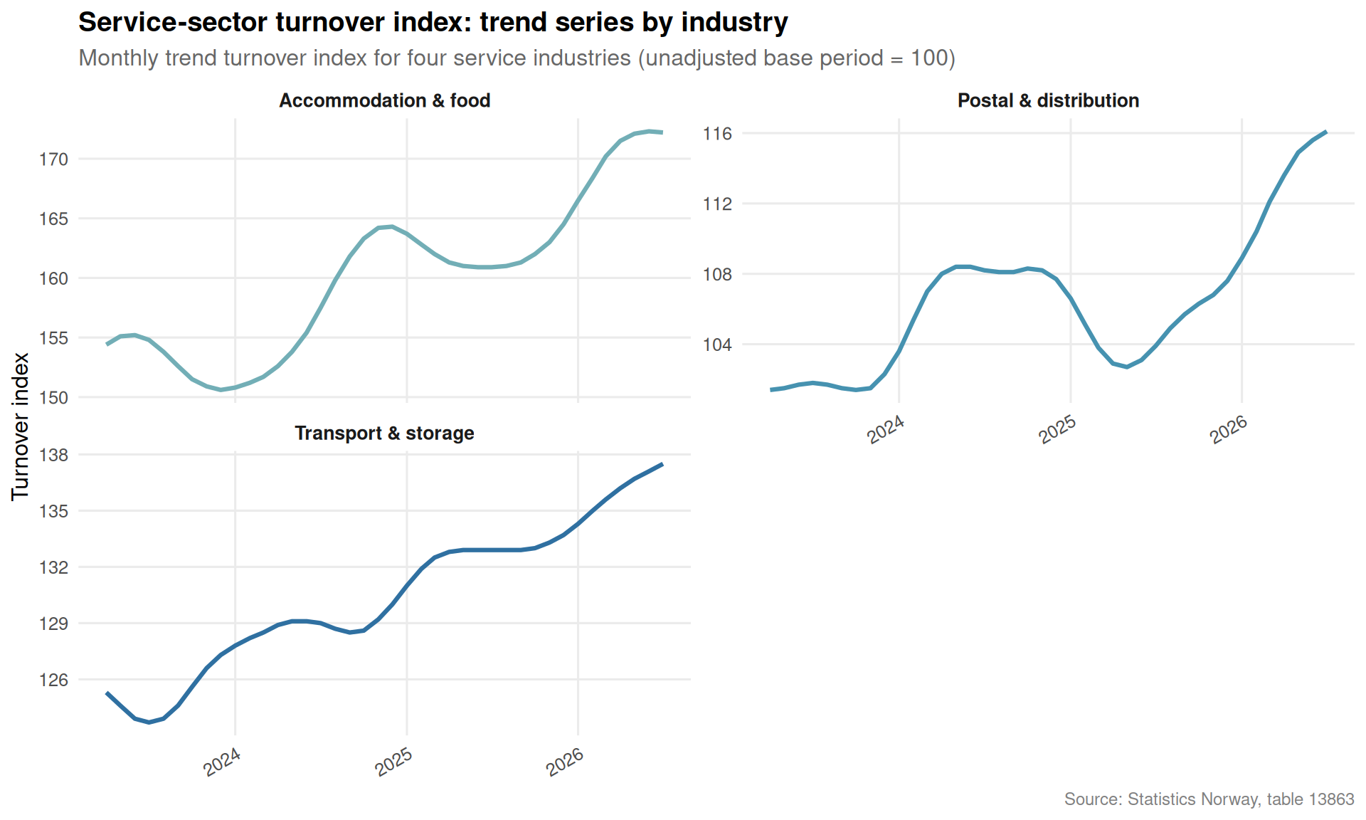
Monthly turnover indices from SSB’s service-sector statistics capture how different industries have fared in real terms. The small-multiples chart below plots the trend series for four key sectors — total services (ex. finance), transport and storage, accommodation and food service, and postal distribution — allowing direct visual comparison of their trajectories.

Code

if (exists("df2_trend") && !is.null(df2_trend) && nrow(df2_trend) > 0) {

  sector_labels <- c(
    "Tjenester ekskl. finansieringsvirksomhet" = "Services excl. finance",
    "Transport og lagring"                     = "Transport & storage",
    "Overnattings- og serveringsvirksomhet"    = "Accommodation & food",
    "Post og distribusjonsvirksomhet"          = "Postal & distribution"
  )

  df2_trend_plot <- df2_trend |>
    mutate(sector_en = recode(.data[["næring"]], !!!sector_labels))

  pal4 <- met.brewer("Hokusai2", n = 4)

  p <- ggplot(df2_trend_plot, aes(x = date, y = value, colour = sector_en)) +
    geom_line(linewidth = 1.1) +
    facet_wrap(~ sector_en, scales = "free_y", ncol = 2) +
    scale_colour_manual(values = pal4) +
    scale_x_date(date_breaks = "1 year", date_labels = "%Y") +
    labs(
      title    = "Service-sector turnover index: trend series by industry",
      subtitle = "Monthly trend turnover index for four service industries (unadjusted base period = 100)",
      caption  = "Source: Statistics Norway, table 13863",
      x = NULL, y = "Turnover index",
      colour = NULL
    ) +
    theme_minimal(base_size = 12) +
    theme(
      legend.position   = "none",
      strip.text        = element_text(face = "bold", size = 10),
      panel.grid.minor  = element_blank(),
      axis.text.x       = element_text(angle = 30, hjust = 1),
      plot.title        = element_text(face = "bold"),
      plot.subtitle     = element_text(colour = "grey40"),
      plot.caption      = element_text(colour = "grey50", size = 9)
    )

  print(p)

  # Data-driven commentary
  latest_date2 <- max(df2_trend_plot$date)
  latest_t2    <- df2_trend_plot |> filter(date == latest_date2)
  top_sector   <- latest_t2[which.max(latest_t2$value), ]
  bot_sector   <- latest_t2[which.min(latest_t2$value), ]

  cat(sprintf(
    "\n\nIn %s, the highest turnover index among the four sectors was recorded by '%s' (index: %.1f), while the lowest was '%s' (index: %.1f).\n\n",
    format(latest_date2, "%B %Y"),
    top_sector$sector_en,
    top_sector$value,
    bot_sector$sector_en,
    bot_sector$value
  ))

} else {
  cat("\n\n*Figure omitted — Statistics Norway returned no data for this series.*\n\n")
}

In July 2026, the highest turnover index among the four sectors was recorded by ‘Accommodation & food’ (index: 172.2), while the lowest was ‘Postal & distribution’ (index: 116.1).

Code

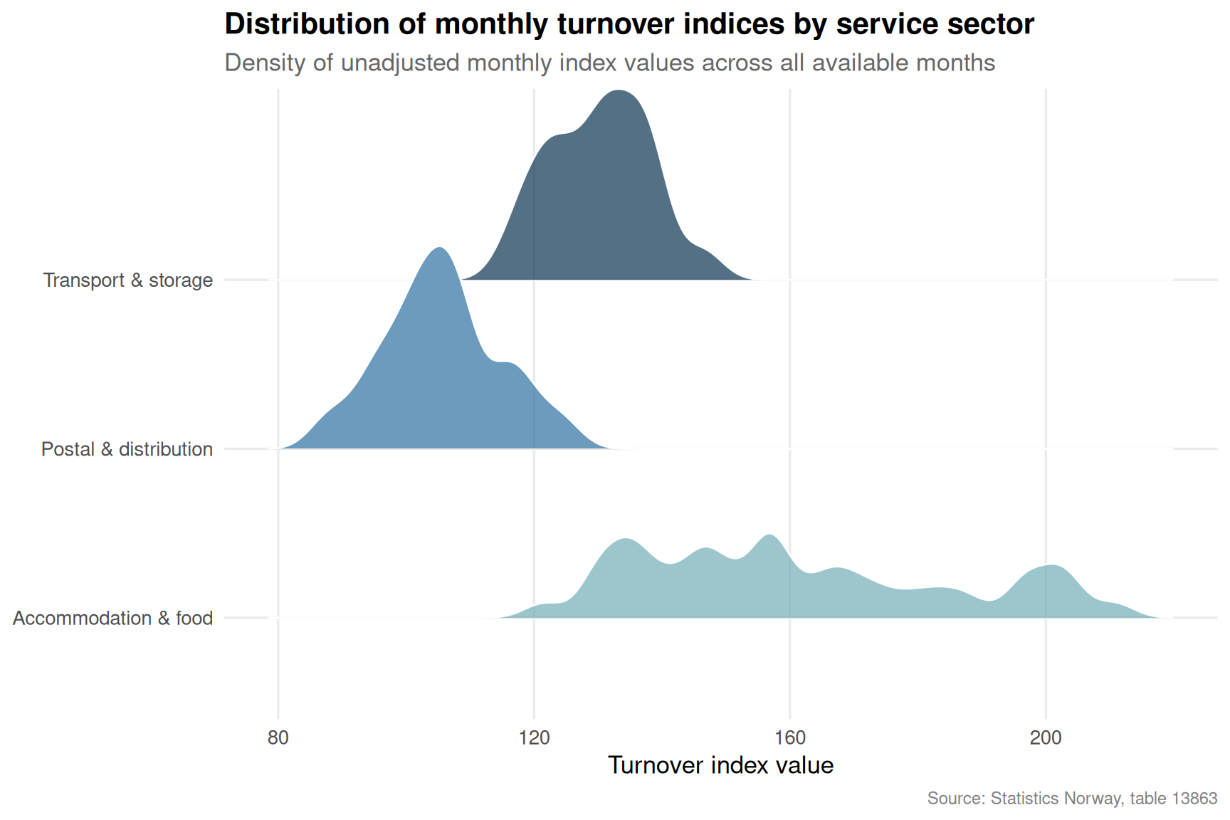
if (exists("df2_unadj") && !is.null(df2_unadj) && nrow(df2_unadj) > 0) {

  sector_labels <- c(
    "Tjenester ekskl. finansieringsvirksomhet" = "Services excl. finance",
    "Transport og lagring"                     = "Transport & storage",
    "Overnattings- og serveringsvirksomhet"    = "Accommodation & food",
    "Post og distribusjonsvirksomhet"          = "Postal & distribution"
  )

  df2_ridge <- df2_unadj |>
    mutate(
      sector_en = recode(.data[["næring"]], !!!sector_labels),
      year      = lubridate::year(date)
    ) |>
    filter(!is.na(value))

  pal_ridge <- met.brewer("Hokusai2", n = length(unique(df2_ridge$sector_en)))

  p <- ggplot(df2_ridge, aes(x = value, y = sector_en, fill = sector_en)) +
    geom_density_ridges(
      alpha       = 0.7,
      scale       = 1.2,
      bandwidth   = 3,
      colour      = "white"
    ) +
    scale_fill_manual(values = pal_ridge) +
    labs(
      title    = "Distribution of monthly turnover indices by service sector",
      subtitle = "Density of unadjusted monthly index values across all available months",
      caption  = "Source: Statistics Norway, table 13863",
      x = "Turnover index value", y = NULL,
      fill = NULL
    ) +
    theme_minimal(base_size = 13) +
    theme(
      legend.position  = "none",
      panel.grid.minor = element_blank(),
      plot.title       = element_text(face = "bold"),
      plot.subtitle    = element_text(colour = "grey40"),
      plot.caption     = element_text(colour = "grey50", size = 9)
    )

  print(p)

  # Data-driven commentary
  sector_stats <- df2_ridge |>
    group_by(sector_en) |>
    summarise(med_val = median(value, na.rm = TRUE), .groups = "drop") |>
    arrange(desc(med_val))

  cat(sprintf(
    "\n\nAcross all available months, '%s' shows the highest median unadjusted turnover index (%.1f), while '%s' records the lowest median (%.1f).\n\n",
    sector_stats$sector_en[1], sector_stats$med_val[1],
    sector_stats$sector_en[nrow(sector_stats)], sector_stats$med_val[nrow(sector_stats)]
  ))

} else {
  cat("\n\n*Figure omitted — Statistics Norway returned no data for this series.*\n\n")
}

Across all available months, ‘Accommodation & food’ shows the highest median unadjusted turnover index (157.0), while ‘Postal & distribution’ records the lowest median (105.1).

Consumer Price Divergence: Which Baskets Are Getting More Expensive

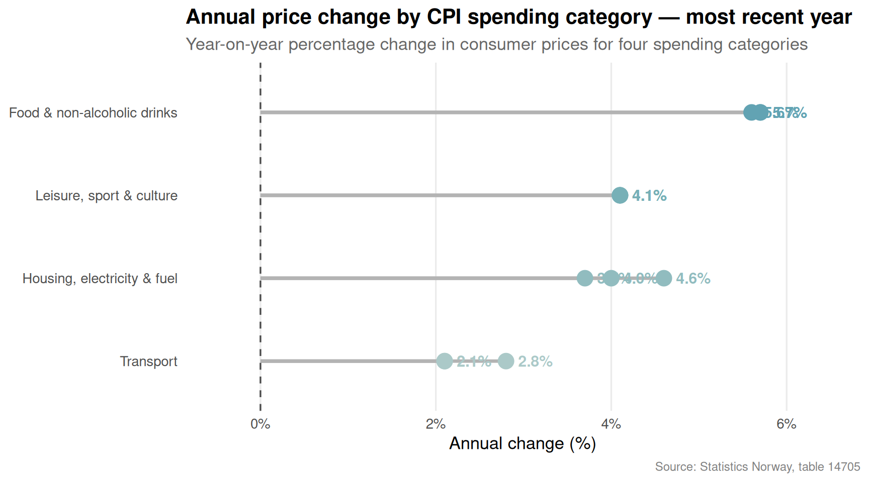
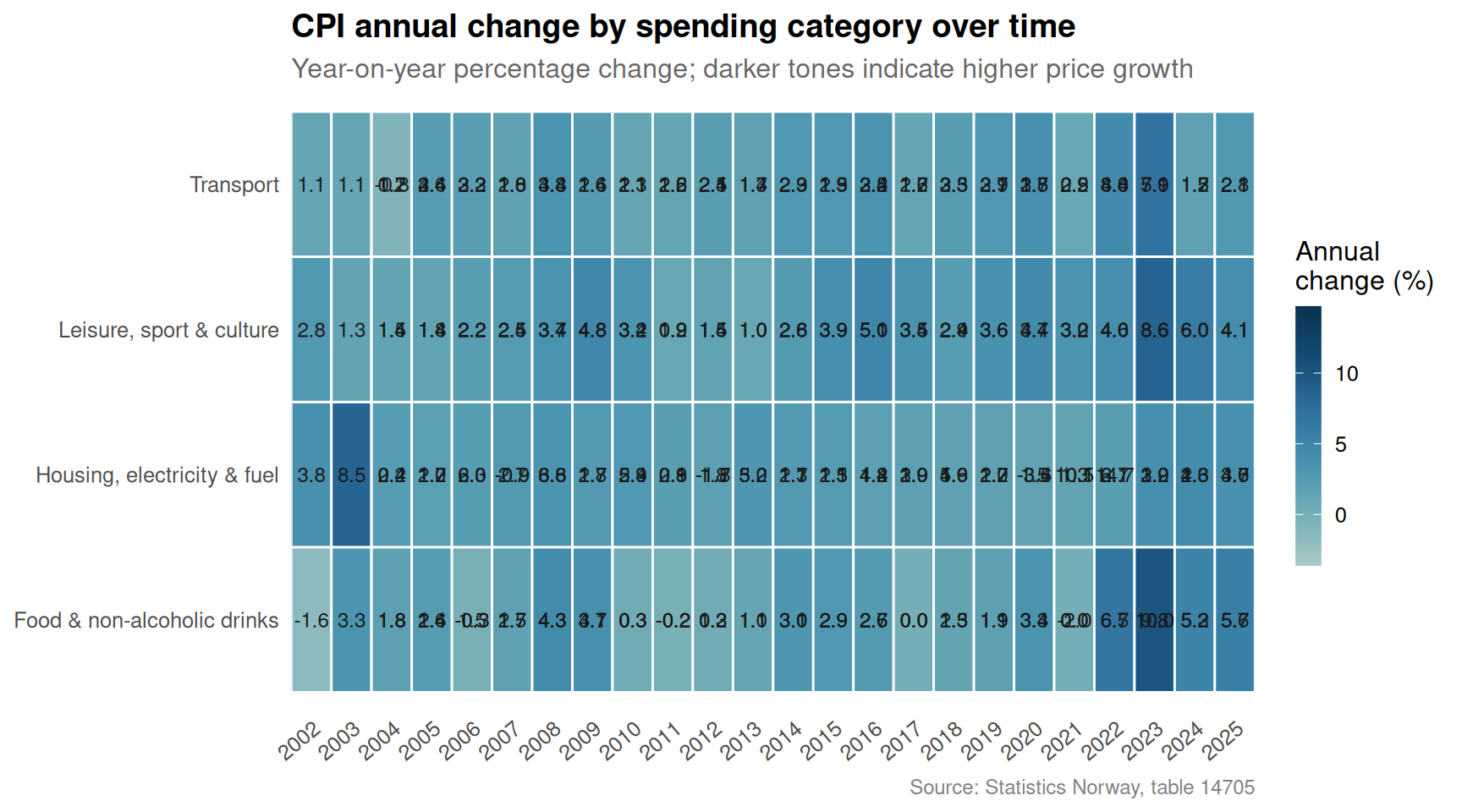
The consumer price index (CPI) broken down by spending category reveals whether the price pressure households feel is concentrated in specific areas of life — food, housing and energy, transport, or leisure and culture. The lollipop chart below shows the most recent annual rate of change for each category, and the heatmap tracks how those rates have evolved year by year.

Code

# CPI wrangling — all derived frames initialised first
df3_yoy        <- NULL
df3_yoy_plot   <- NULL
df3_lollipop   <- NULL
df3_heatmap    <- NULL
df3_index      <- NULL

if (!is.null(df3) && nrow(df3) > 0) {

  df3_yoy <- df3 |>
    filter(
      .data[["vare- og tjenestegruppe"]] %in% c(
        "Matvarer og alkoholfrie drikkevarer",
        "Bolig, elektrisitet og brensel",
        "Transport",
        "Fritid, sport og kultur"
      ),
      .data[["statistikkvariabel"]] == "Årsendring (prosent)"
    )

  if (nrow(df3_yoy) == 0) {
    message("df3_yoy empty. series values: ",
            paste(head(unique(df3[["vare- og tjenestegruppe"]]), 15), collapse = ", "))
    message("measure values: ",
            paste(head(unique(df3[["statistikkvariabel"]]), 15), collapse = ", "))
    df3_yoy <- NULL
  }

  cat_labels <- c(
    "Matvarer og alkoholfrie drikkevarer" = "Food & non-alcoholic drinks",
    "Bolig, elektrisitet og brensel"      = "Housing, electricity & fuel",
    "Transport"                           = "Transport",
    "Fritid, sport og kultur"             = "Leisure, sport & culture"
  )

  df3_yoy_plot <- if (!is.null(df3_yoy) && nrow(df3_yoy) > 0) {
    df3_yoy |>
      mutate(cat_en = recode(.data[["vare- og tjenestegruppe"]], !!!cat_labels))
  } else NULL

  # Lollipop: most recent year
  df3_lollipop <- if (!is.null(df3_yoy_plot) && nrow(df3_yoy_plot) > 0) {
    df3_yoy_plot |>
      filter(date == max(date))
  } else NULL

  # Heatmap: all years
  df3_heatmap <- df3_yoy_plot

  # Index series
  df3_index <- df3 |>
    filter(
      .data[["vare- og tjenestegruppe"]] %in% c(
        "Matvarer og alkoholfrie drikkevarer",
        "Bolig, elektrisitet og brensel",
        "Transport",
        "Fritid, sport og kultur"
      ),
      .data[["statistikkvariabel"]] == "Indeks (2025=100)"
    ) |>
    mutate(cat_en = recode(.data[["vare- og tjenestegruppe"]], !!!cat_labels))
}

Code

if (exists("df3_lollipop") && !is.null(df3_lollipop) && nrow(df3_lollipop) > 0) {

  pal_lol <- met.brewer("Hokusai2", n = nrow(df3_lollipop))

  df3_lol_ordered <- df3_lollipop |>
    arrange(value) |>
    mutate(cat_en = factor(cat_en, levels = unique(cat_en))) # fixed: use unique() to avoid duplicate factor levels

  p <- ggplot(df3_lol_ordered, aes(x = value, y = cat_en, colour = cat_en)) +
    geom_segment(aes(x = 0, xend = value, y = cat_en, yend = cat_en),
                 linewidth = 1.2, colour = "grey70") +
    geom_point(size = 5) +
    geom_vline(xintercept = 0, colour = "grey30", linewidth = 0.6, linetype = "dashed") +
    geom_text(aes(label = sprintf("%.1f%%", value)),
              hjust = ifelse(df3_lol_ordered$value >= 0, -0.35, 1.35),
              size = 4, fontface = "bold") +
    scale_colour_manual(values = pal_lol) +
    scale_x_continuous(
      labels = function(x) paste0(x, "%"),
      expand = expansion(mult = c(0.15, 0.2))
    ) +
    labs(
      title    = "Annual price change by CPI spending category — most recent year",
      subtitle = "Year-on-year percentage change in consumer prices for four spending categories",
      caption  = "Source: Statistics Norway, table 14705",
      x = "Annual change (%)", y = NULL
    ) +
    theme_minimal(base_size = 13) +
    theme(
      legend.position  = "none",
      panel.grid.major.y = element_blank(),
      panel.grid.minor   = element_blank(),
      plot.title         = element_text(face = "bold"),
      plot.subtitle      = element_text(colour = "grey40"),
      plot.caption       = element_text(colour = "grey50", size = 9)
    )

  print(p) # fixed: explicit print to ensure figure renders

  top_cat <- df3_lol_ordered[which.max(df3_lol_ordered$value), ]
  bot_cat <- df3_lol_ordered[which.min(df3_lol_ordered$value), ]
  yr_lol  <- format(max(df3_lollipop$date), "%Y")

  cat(sprintf(
    "\n\nIn %s, the sharpest annual price increase among the four categories was in '%s' (%.1f%%), while '%s' saw the smallest change (%.1f%%).\n\n",
    yr_lol,
    top_cat$cat_en, top_cat$value,
    bot_cat$cat_en, bot_cat$value
  ))

} else {
  cat("\n\n*Figure omitted — Statistics Norway returned no data for this series.*\n\n")
}

In 2025, the sharpest annual price increase among the four categories was in ‘Food & non-alcoholic drinks’ (5.7%), while ‘Transport’ saw the smallest change (2.1%).

Code

if (exists("df3_heatmap") && !is.null(df3_heatmap) && nrow(df3_heatmap) > 0) {

  df3_hm <- df3_heatmap |>
    mutate(year = lubridate::year(date)) |>
    filter(!is.na(value))

  p <- ggplot(df3_hm, aes(x = year, y = cat_en, fill = value)) +
    geom_tile(colour = "white", linewidth = 0.5) +
    geom_text(aes(label = sprintf("%.1f", value)),
              size = 3.2, colour = "grey10") +
    scale_fill_gradientn(
      colours  = met.brewer("Hokusai2", n = 9),
      name     = "Annual\nchange (%)",
      guide    = guide_colourbar(barwidth = 0.8, barheight = 8)
    ) +
    scale_x_continuous(breaks = unique(df3_hm$year), expand = expansion(0)) +
    labs(
      title    = "CPI annual change by spending category over time",
      subtitle = "Year-on-year percentage change; darker tones indicate higher price growth",
      caption  = "Source: Statistics Norway, table 14705",
      x = NULL, y = NULL
    ) +
    theme_minimal(base_size = 12) +
    theme(
      panel.grid   = element_blank(),
      axis.text.x  = element_text(angle = 40, hjust = 1),
      plot.title   = element_text(face = "bold"),
      plot.subtitle = element_text(colour = "grey40"),
      plot.caption = element_text(colour = "grey50", size = 9)
    )

  print(p)

  # Most volatile category
  cat_volatility <- df3_hm |>
    group_by(cat_en) |>
    summarise(sd_val = sd(value, na.rm = TRUE), .groups = "drop") |>
    arrange(desc(sd_val))

  cat(sprintf(
    "\n\nOver the full period, '%s' shows the highest year-to-year price volatility (standard deviation: %.1f percentage points), suggesting it has been the most unpredictable spending category for Norwegian households.\n\n",
    cat_volatility$cat_en[1], cat_volatility$sd_val[1]
  ))

} else {
  cat("\n\n*Figure omitted — Statistics Norway returned no data for this series.*\n\n")
}

Over the full period, ‘Housing, electricity & fuel’ shows the highest year-to-year price volatility (standard deviation: 3.0 percentage points), suggesting it has been the most unpredictable spending category for Norwegian households.

Key Findings

Code

bullets <- character(0)

# df1 findings
if (exists("df1_area") && !is.null(df1_area) && nrow(df1_area) > 0) {
  latest_d1 <- max(df1_area$date)
  row_g <- df1_area |>
    filter(.data[["makrostørrelse"]] == "Varekonsum", date == latest_d1)
  row_s <- df1_area |>
    filter(.data[["makrostørrelse"]] == "Tjenestekonsum", date == latest_d1)

  if (nrow(row_g) > 0 && nrow(row_s) > 0) {
    diff_pct <- (row_s$value - row_g$value) / row_g$value * 100
    bullets <- c(bullets, sprintf(
      "- **Household consumption (quarterly, fixed 2023 prices):** In %s, services consumption exceeded goods consumption by %.1f%% in volume terms (NOK %.1f bn vs NOK %.1f bn).",
      format(latest_d1, "%Y Q%q"),
      diff_pct,
      row_s$value / 1000,
      row_g$value / 1000
    ))
  }
}

# df2 findings
if (exists("df2_trend") && !is.null(df2_trend) && nrow(df2_trend) > 0) {
  sector_labels_f <- c(
    "Tjenester ekskl. finansieringsvirksomhet" = "Services excl. finance",
    "Transport og lagring"                     = "Transport & storage",
    "Overnattings- og serveringsvirksomhet"    = "Accommodation & food",
    "Post og distribusjonsvirksomhet"          = "Postal & distribution"
  )
  df2_latest <- df2_trend |>
    filter(date == max(date)) |>
    mutate(sector_en = recode(.data[["næring"]], !!!sector_labels_f))

  if (nrow(df2_latest) > 0) {
    top_s <- df2_latest[which.max(df2_latest$value), ]
    bot_s <- df2_latest[which.min(df2_latest$value), ]
    bullets <- c(bullets, sprintf(
      "- **Service-sector turnover (monthly trend index):** As of %s, '%s' posted the highest trend turnover index (%.1f) while '%s' recorded the lowest (%.1f).",
      format(max(df2_trend$date), "%B %Y"),
      top_s$sector_en, top_s$value,
      bot_s$sector_en, bot_s$value
    ))
  }
}

# df3 findings
if (exists("df3_lollipop") && !is.null(df3_lollipop) && nrow(df3_lollipop) > 0) {
  top3 <- df3_lollipop[which.max(df3_lollipop$value), ]
  bot3 <- df3_lollipop[which.min(df3_lollipop$value), ]
  bullets <- c(bullets, sprintf(
    "- **Consumer price changes by spending category (%s):** The steepest annual price rise was in '%s' (+%.1f%%) and the most moderate in '%s' (%.1f%%).",
    format(max(df3_lollipop$date), "%Y"),
    top3$cat_en, top3$value,
    bot3$cat_en, bot3$value
  ))
}

if (length(bullets) > 0) {
  cat("### Key findings\n\n")
  cat(paste(bullets, collapse = "\n\n"))
  cat("\n\n")
}

Key findings

Service-sector turnover (monthly trend index): As of July 2026, ‘Accommodation & food’ posted the highest trend turnover index (172.2) while ‘Postal & distribution’ recorded the lowest (116.1).
Consumer price changes by spending category (2025): The steepest annual price rise was in ‘Food & non-alcoholic drinks’ (+5.7%) and the most moderate in ‘Transport’ (2.1%).

Closing Reflection

The picture that emerges from these three datasets is one of structural divergence rather than a single narrative of boom or bust. Norwegian household spending is shaped by forces that do not move in unison: quarterly national accounts capture the volume of what people actually buy; monthly turnover indices reveal how individual service industries are holding up in practice; and annual consumer price breakdowns show where the cost squeeze is concentrated. Together, they suggest that the Norwegian consumer story in 2026 is a story of segmentation — different sectors, different price paths, and different pressures bearing down on different kinds of spending. Policy responses that treat household consumption as a monolithic aggregate risk misreading the underlying dynamics entirely.

--- title: "Norway's 2026 Consumption Divergence: How Services Inflation Stalled Spending While Retail Shelves Held Firm" description: "Quarterly household spending, monthly service-sector turnover, and annual consumer price indices reveal how Norwegian consumers are navigating a fractured cost landscape." date: "2026-08-08" categories: [SSB, consumption, inflation, services, household spending] --- Norwegian households are caught between two forces pulling in opposite directions: persistent price pressures in services and housing that erode purchasing power, and a goods market that has shown surprising resilience. Understanding how these dynamics interact across spending categories, service industries, and consumer price baskets is essential for reading the state of Norway's economy in 2026. This post draws on three SSB datasets — quarterly national accounts consumption data, monthly service-sector turnover indices, and annual consumer price index components — to trace the divergence. ```{r setup} knitr::opts_chunk$set(echo = TRUE, warning = FALSE, message = FALSE, error = TRUE) library(tidyverse) library(lubridate) library(PxWebApiData) library(scales) library(ggridges) library(MetBrewer) df1 <- NULL tryCatch({ raw <- ApiData( "https://data.ssb.no/api/v0/no/table/09190", Makrost = TRUE, Tid = list(filter = "top", values = 40) ) tmp <- raw[[1]] time_col <- "kvartal" value_col <- "value" series_col <- "makrostørrelse" measure_col <- "statistikkvariabel" df1 <- tmp |> mutate( value = as.numeric(.data[[value_col]]), time_str = .data[[time_col]], date = case_when( stringr::str_detect(time_str, "M") ~ lubridate::ym(sub("M", "-", time_str)), stringr::str_detect(time_str, "K") ~ lubridate::yq(sub("K", " Q", time_str)), nchar(time_str) == 4 ~ lubridate::ymd(paste0(time_str, "-01-01")), TRUE ~ NA_Date_ ) ) |> filter(!is.na(value), !is.na(date)) }, error = function(e) message("Fetch failed: ", e$message)) if (is.null(df1) || nrow(df1) == 0) { message("No data returned"); df1 <- NULL } df2 <- NULL tryCatch({ raw <- ApiData( "https://data.ssb.no/api/v0/no/table/13863", NACE = TRUE, ContentsCode = TRUE, Tid = list(filter = "top", values = 40) ) tmp <- raw[[1]] time_col <- "måned" value_col <- "value" series_col <- "næring" measure_col <- "statistikkvariabel" df2 <- tmp |> mutate( value = as.numeric(.data[[value_col]]), time_str = .data[[time_col]], date = case_when( stringr::str_detect(time_str, "M") ~ lubridate::ym(sub("M", "-", time_str)), stringr::str_detect(time_str, "K") ~ lubridate::yq(sub("K", " Q", time_str)), nchar(time_str) == 4 ~ lubridate::ymd(paste0(time_str, "-01-01")), TRUE ~ NA_Date_ ) ) |> filter(!is.na(value), !is.na(date)) }, error = function(e) message("Fetch failed: ", e$message)) if (is.null(df2) || nrow(df2) == 0) { message("No data returned"); df2 <- NULL } df3 <- NULL tryCatch({ raw <- ApiData( "https://data.ssb.no/api/v0/no/table/14705", KPIavledetSerie = TRUE, VareTjenesteGrp = TRUE, Tid = list(filter = "top", values = 40) ) tmp <- raw[[1]] time_col <- "år" value_col <- "value" series_col <- "vare- og tjenestegruppe" measure_col <- "statistikkvariabel" df3 <- tmp |> mutate( value = as.numeric(.data[[value_col]]), time_str = .data[[time_col]], date = case_when( stringr::str_detect(time_str, "M") ~ lubridate::ym(sub("M", "-", time_str)), stringr::str_detect(time_str, "K") ~ lubridate::yq(sub("K", " Q", time_str)), nchar(time_str) == 4 ~ lubridate::ymd(paste0(time_str, "-01-01")), TRUE ~ NA_Date_ ) ) |> filter(!is.na(value), !is.na(date)) }, error = function(e) message("Fetch failed: ", e$message)) if (is.null(df3) || nrow(df3) == 0) { message("No data returned"); df3 <- NULL } ``` ## Household Consumption: Goods vs. Services in the National Accounts Norway's quarterly national accounts distinguish sharply between what households spend on physical goods and what they pay for services. In an environment of persistent services inflation, this split carries growing analytical weight. The area chart below plots real-terms consumption for goods and services over the most recent ten years of quarterly data, tracking how the two components have moved relative to each other. ```{r wrangle-df1} # All derived data frames initialised up front df1_vol <- NULL df1_area <- NULL df1_yoy <- NULL df1_yoy_latest <- NULL if (!is.null(df1) && nrow(df1) > 0) { # Fixed-price volume for goods vs services consumption df1_vol <- df1 |> filter( .data[["makrostørrelse"]] %in% c("Varekonsum", "Tjenestekonsum"), .data[["statistikkvariabel"]] == "Faste 2023-priser (mill. kr)" ) if (nrow(df1_vol) == 0) { message("df1_vol empty. series values: ", paste(head(unique(df1[["makrostørrelse"]]), 15), collapse = ", ")) df1_vol <- NULL } # For area chart: keep last 40 quarters, both components df1_area <- if (!is.null(df1_vol) && nrow(df1_vol) > 0) { df1_vol |> arrange(date) |> group_by(.data[["makrostørrelse"]]) |> slice_tail(n = 40) |> ungroup() } else NULL # Year-over-year volume change df1_yoy <- df1 |> filter( .data[["makrostørrelse"]] %in% c("Varekonsum", "Tjenestekonsum", "Konsum i husholdninger"), .data[["statistikkvariabel"]] == "Volumendring fra samme periode året før (prosent)" ) df1_yoy_latest <- if (!is.null(df1_yoy) && nrow(df1_yoy) > 0) { df1_yoy |> filter(date == max(date)) } else NULL } ``` ```{r plot-area-consumption} #| fig-height: 5 #| fig-width: 9 #| fig-show: asis #| dev: "png" #| results: asis if (exists("df1_area") && !is.null(df1_area) && nrow(df1_area) > 0) { pal <- met.brewer("Hokusai2", n = 2) series_labels <- c( "Varekonsum" = "Goods consumption", "Tjenestekonsum" = "Services consumption" ) df1_area_plot <- df1_area |> mutate(series_en = recode(.data[["makrostørrelse"]], !!!series_labels)) p <- ggplot(df1_area_plot, aes(x = date, y = value / 1000, fill = series_en, colour = series_en)) + geom_area(alpha = 0.55, position = "identity") + geom_line(linewidth = 0.7) + scale_fill_manual(values = pal) + scale_colour_manual(values = pal) + scale_x_date(date_breaks = "2 years", date_labels = "%Y") + scale_y_continuous(labels = comma_format(suffix = " bn kr")) + labs( title = "Household goods and services consumption, fixed 2023 prices", subtitle = "Quarterly volume of goods and services spending, national accounts (billion NOK)", caption = "Source: Statistics Norway, table 09190", x = NULL, y = "Billion NOK (fixed 2023 prices)", fill = NULL, colour = NULL ) + theme_minimal(base_size = 13) + theme( legend.position = "top", panel.grid.minor = element_blank(), plot.title = element_text(face = "bold"), plot.subtitle = element_text(colour = "grey40"), plot.caption = element_text(colour = "grey50", size = 9) ) print(p) # fixed: explicit print to ensure figure renders # Data-driven commentary latest_date <- max(df1_area_plot$date) latest_vals <- df1_area_plot |> filter(date == latest_date) goods_val <- latest_vals |> filter(.data[["makrostørrelse"]] == "Varekonsum") |> pull(value) svc_val <- latest_vals |> filter(.data[["makrostørrelse"]] == "Tjenestekonsum") |> pull(value) if (length(goods_val) > 0 && length(svc_val) > 0) { cat(sprintf( "\n\nIn the most recent quarter (%s), goods consumption stood at NOK %.1f billion and services consumption at NOK %.1f billion (both in fixed 2023 prices).\n\n", format(latest_date, "%Y Q%q"), goods_val / 1000, svc_val / 1000 )) } } else { cat("\n\n*Figure omitted — Statistics Norway returned no data for this series.*\n\n") } ``` ```{r wrangle-df2} # Service-sector turnover wrangling — all derived frames initialised first df2_trend <- NULL df2_sector4 <- NULL df2_unadj <- NULL if (!is.null(df2) && nrow(df2) > 0) { # Trend series for small-multiples facet df2_trend <- df2 |> filter( .data[["næring"]] %in% c( "Tjenester ekskl. finansieringsvirksomhet", "Transport og lagring", "Overnattings- og serveringsvirksomhet", "Post og distribusjonsvirksomhet" ), .data[["statistikkvariabel"]] == "Omsetningsindeks. Trend" ) if (nrow(df2_trend) == 0) { message("df2_trend empty. n.ring values: ", paste(head(unique(df2[["næring"]]), 15), collapse = ", ")) message("statistikkvariabel values: ", paste(head(unique(df2[["statistikkvariabel"]]), 15), collapse = ", ")) df2_trend <- NULL } # Unadjusted for ridgeline df2_unadj <- df2 |> filter( .data[["næring"]] %in% c( "Tjenester ekskl. finansieringsvirksomhet", "Transport og lagring", "Overnattings- og serveringsvirksomhet", "Post og distribusjonsvirksomhet" ), .data[["statistikkvariabel"]] == "Omsetningsindeks. Ujustert" ) if (nrow(df2_unadj) == 0) { df2_unadj <- NULL } } ``` ## Service-Sector Turnover: Where the Pressure Lives Monthly turnover indices from SSB's service-sector statistics capture how different industries have fared in real terms. The small-multiples chart below plots the trend series for four key sectors — total services (ex. finance), transport and storage, accommodation and food service, and postal distribution — allowing direct visual comparison of their trajectories. ```{r plot-small-multiples-services} #| fig-height: 6 #| fig-width: 10 #| fig-show: asis #| dev: "png" #| results: asis if (exists("df2_trend") && !is.null(df2_trend) && nrow(df2_trend) > 0) { sector_labels <- c( "Tjenester ekskl. finansieringsvirksomhet" = "Services excl. finance", "Transport og lagring" = "Transport & storage", "Overnattings- og serveringsvirksomhet" = "Accommodation & food", "Post og distribusjonsvirksomhet" = "Postal & distribution" ) df2_trend_plot <- df2_trend |> mutate(sector_en = recode(.data[["næring"]], !!!sector_labels)) pal4 <- met.brewer("Hokusai2", n = 4) p <- ggplot(df2_trend_plot, aes(x = date, y = value, colour = sector_en)) + geom_line(linewidth = 1.1) + facet_wrap(~ sector_en, scales = "free_y", ncol = 2) + scale_colour_manual(values = pal4) + scale_x_date(date_breaks = "1 year", date_labels = "%Y") + labs( title = "Service-sector turnover index: trend series by industry", subtitle = "Monthly trend turnover index for four service industries (unadjusted base period = 100)", caption = "Source: Statistics Norway, table 13863", x = NULL, y = "Turnover index", colour = NULL ) + theme_minimal(base_size = 12) + theme( legend.position = "none", strip.text = element_text(face = "bold", size = 10), panel.grid.minor = element_blank(), axis.text.x = element_text(angle = 30, hjust = 1), plot.title = element_text(face = "bold"), plot.subtitle = element_text(colour = "grey40"), plot.caption = element_text(colour = "grey50", size = 9) ) print(p) # Data-driven commentary latest_date2 <- max(df2_trend_plot$date) latest_t2 <- df2_trend_plot |> filter(date == latest_date2) top_sector <- latest_t2[which.max(latest_t2$value), ] bot_sector <- latest_t2[which.min(latest_t2$value), ] cat(sprintf( "\n\nIn %s, the highest turnover index among the four sectors was recorded by '%s' (index: %.1f), while the lowest was '%s' (index: %.1f).\n\n", format(latest_date2, "%B %Y"), top_sector$sector_en, top_sector$value, bot_sector$sector_en, bot_sector$value )) } else { cat("\n\n*Figure omitted — Statistics Norway returned no data for this series.*\n\n") } ``` ```{r plot-ridgeline-services} #| fig-height: 6 #| fig-width: 9 #| fig-show: asis #| dev: "png" #| results: asis if (exists("df2_unadj") && !is.null(df2_unadj) && nrow(df2_unadj) > 0) { sector_labels <- c( "Tjenester ekskl. finansieringsvirksomhet" = "Services excl. finance", "Transport og lagring" = "Transport & storage", "Overnattings- og serveringsvirksomhet" = "Accommodation & food", "Post og distribusjonsvirksomhet" = "Postal & distribution" ) df2_ridge <- df2_unadj |> mutate( sector_en = recode(.data[["næring"]], !!!sector_labels), year = lubridate::year(date) ) |> filter(!is.na(value)) pal_ridge <- met.brewer("Hokusai2", n = length(unique(df2_ridge$sector_en))) p <- ggplot(df2_ridge, aes(x = value, y = sector_en, fill = sector_en)) + geom_density_ridges( alpha = 0.7, scale = 1.2, bandwidth = 3, colour = "white" ) + scale_fill_manual(values = pal_ridge) + labs( title = "Distribution of monthly turnover indices by service sector", subtitle = "Density of unadjusted monthly index values across all available months", caption = "Source: Statistics Norway, table 13863", x = "Turnover index value", y = NULL, fill = NULL ) + theme_minimal(base_size = 13) + theme( legend.position = "none", panel.grid.minor = element_blank(), plot.title = element_text(face = "bold"), plot.subtitle = element_text(colour = "grey40"), plot.caption = element_text(colour = "grey50", size = 9) ) print(p) # Data-driven commentary sector_stats <- df2_ridge |> group_by(sector_en) |> summarise(med_val = median(value, na.rm = TRUE), .groups = "drop") |> arrange(desc(med_val)) cat(sprintf( "\n\nAcross all available months, '%s' shows the highest median unadjusted turnover index (%.1f), while '%s' records the lowest median (%.1f).\n\n", sector_stats$sector_en[1], sector_stats$med_val[1], sector_stats$sector_en[nrow(sector_stats)], sector_stats$med_val[nrow(sector_stats)] )) } else { cat("\n\n*Figure omitted — Statistics Norway returned no data for this series.*\n\n") } ``` ## Consumer Price Divergence: Which Baskets Are Getting More Expensive The consumer price index (CPI) broken down by spending category reveals whether the price pressure households feel is concentrated in specific areas of life — food, housing and energy, transport, or leisure and culture. The lollipop chart below shows the most recent annual rate of change for each category, and the heatmap tracks how those rates have evolved year by year. ```{r wrangle-df3} # CPI wrangling — all derived frames initialised first df3_yoy <- NULL df3_yoy_plot <- NULL df3_lollipop <- NULL df3_heatmap <- NULL df3_index <- NULL if (!is.null(df3) && nrow(df3) > 0) { df3_yoy <- df3 |> filter( .data[["vare- og tjenestegruppe"]] %in% c( "Matvarer og alkoholfrie drikkevarer", "Bolig, elektrisitet og brensel", "Transport", "Fritid, sport og kultur" ), .data[["statistikkvariabel"]] == "Årsendring (prosent)" ) if (nrow(df3_yoy) == 0) { message("df3_yoy empty. series values: ", paste(head(unique(df3[["vare- og tjenestegruppe"]]), 15), collapse = ", ")) message("measure values: ", paste(head(unique(df3[["statistikkvariabel"]]), 15), collapse = ", ")) df3_yoy <- NULL } cat_labels <- c( "Matvarer og alkoholfrie drikkevarer" = "Food & non-alcoholic drinks", "Bolig, elektrisitet og brensel" = "Housing, electricity & fuel", "Transport" = "Transport", "Fritid, sport og kultur" = "Leisure, sport & culture" ) df3_yoy_plot <- if (!is.null(df3_yoy) && nrow(df3_yoy) > 0) { df3_yoy |> mutate(cat_en = recode(.data[["vare- og tjenestegruppe"]], !!!cat_labels)) } else NULL # Lollipop: most recent year df3_lollipop <- if (!is.null(df3_yoy_plot) && nrow(df3_yoy_plot) > 0) { df3_yoy_plot |> filter(date == max(date)) } else NULL # Heatmap: all years df3_heatmap <- df3_yoy_plot # Index series df3_index <- df3 |> filter( .data[["vare- og tjenestegruppe"]] %in% c( "Matvarer og alkoholfrie drikkevarer", "Bolig, elektrisitet og brensel", "Transport", "Fritid, sport og kultur" ), .data[["statistikkvariabel"]] == "Indeks (2025=100)" ) |> mutate(cat_en = recode(.data[["vare- og tjenestegruppe"]], !!!cat_labels)) } ``` ```{r plot-lollipop-cpi} #| fig-height: 5 #| fig-width: 9 #| fig-show: asis #| dev: "png" #| results: asis if (exists("df3_lollipop") && !is.null(df3_lollipop) && nrow(df3_lollipop) > 0) { pal_lol <- met.brewer("Hokusai2", n = nrow(df3_lollipop)) df3_lol_ordered <- df3_lollipop |> arrange(value) |> mutate(cat_en = factor(cat_en, levels = unique(cat_en))) # fixed: use unique() to avoid duplicate factor levels p <- ggplot(df3_lol_ordered, aes(x = value, y = cat_en, colour = cat_en)) + geom_segment(aes(x = 0, xend = value, y = cat_en, yend = cat_en), linewidth = 1.2, colour = "grey70") + geom_point(size = 5) + geom_vline(xintercept = 0, colour = "grey30", linewidth = 0.6, linetype = "dashed") + geom_text(aes(label = sprintf("%.1f%%", value)), hjust = ifelse(df3_lol_ordered$value >= 0, -0.35, 1.35), size = 4, fontface = "bold") + scale_colour_manual(values = pal_lol) + scale_x_continuous( labels = function(x) paste0(x, "%"), expand = expansion(mult = c(0.15, 0.2)) ) + labs( title = "Annual price change by CPI spending category — most recent year", subtitle = "Year-on-year percentage change in consumer prices for four spending categories", caption = "Source: Statistics Norway, table 14705", x = "Annual change (%)", y = NULL ) + theme_minimal(base_size = 13) + theme( legend.position = "none", panel.grid.major.y = element_blank(), panel.grid.minor = element_blank(), plot.title = element_text(face = "bold"), plot.subtitle = element_text(colour = "grey40"), plot.caption = element_text(colour = "grey50", size = 9) ) print(p) # fixed: explicit print to ensure figure renders top_cat <- df3_lol_ordered[which.max(df3_lol_ordered$value), ] bot_cat <- df3_lol_ordered[which.min(df3_lol_ordered$value), ] yr_lol <- format(max(df3_lollipop$date), "%Y") cat(sprintf( "\n\nIn %s, the sharpest annual price increase among the four categories was in '%s' (%.1f%%), while '%s' saw the smallest change (%.1f%%).\n\n", yr_lol, top_cat$cat_en, top_cat$value, bot_cat$cat_en, bot_cat$value )) } else { cat("\n\n*Figure omitted — Statistics Norway returned no data for this series.*\n\n") } ``` ```{r plot-heatmap-cpi} #| fig-height: 5 #| fig-width: 9 #| fig-show: asis #| dev: "png" #| results: asis if (exists("df3_heatmap") && !is.null(df3_heatmap) && nrow(df3_heatmap) > 0) { df3_hm <- df3_heatmap |> mutate(year = lubridate::year(date)) |> filter(!is.na(value)) p <- ggplot(df3_hm, aes(x = year, y = cat_en, fill = value)) + geom_tile(colour = "white", linewidth = 0.5) + geom_text(aes(label = sprintf("%.1f", value)), size = 3.2, colour = "grey10") + scale_fill_gradientn( colours = met.brewer("Hokusai2", n = 9), name = "Annual\nchange (%)", guide = guide_colourbar(barwidth = 0.8, barheight = 8) ) + scale_x_continuous(breaks = unique(df3_hm$year), expand = expansion(0)) + labs( title = "CPI annual change by spending category over time", subtitle = "Year-on-year percentage change; darker tones indicate higher price growth", caption = "Source: Statistics Norway, table 14705", x = NULL, y = NULL ) + theme_minimal(base_size = 12) + theme( panel.grid = element_blank(), axis.text.x = element_text(angle = 40, hjust = 1), plot.title = element_text(face = "bold"), plot.subtitle = element_text(colour = "grey40"), plot.caption = element_text(colour = "grey50", size = 9) ) print(p) # Most volatile category cat_volatility <- df3_hm |> group_by(cat_en) |> summarise(sd_val = sd(value, na.rm = TRUE), .groups = "drop") |> arrange(desc(sd_val)) cat(sprintf( "\n\nOver the full period, '%s' shows the highest year-to-year price volatility (standard deviation: %.1f percentage points), suggesting it has been the most unpredictable spending category for Norwegian households.\n\n", cat_volatility$cat_en[1], cat_volatility$sd_val[1] )) } else { cat("\n\n*Figure omitted — Statistics Norway returned no data for this series.*\n\n") } ``` ## Key Findings ```{r key-findings} #| results: asis bullets <- character(0) # df1 findings if (exists("df1_area") && !is.null(df1_area) && nrow(df1_area) > 0) { latest_d1 <- max(df1_area$date) row_g <- df1_area |> filter(.data[["makrostørrelse"]] == "Varekonsum", date == latest_d1) row_s <- df1_area |> filter(.data[["makrostørrelse"]] == "Tjenestekonsum", date == latest_d1) if (nrow(row_g) > 0 && nrow(row_s) > 0) { diff_pct <- (row_s$value - row_g$value) / row_g$value * 100 bullets <- c(bullets, sprintf( "- **Household consumption (quarterly, fixed 2023 prices):** In %s, services consumption exceeded goods consumption by %.1f%% in volume terms (NOK %.1f bn vs NOK %.1f bn).", format(latest_d1, "%Y Q%q"), diff_pct, row_s$value / 1000, row_g$value / 1000 )) } } # df2 findings if (exists("df2_trend") && !is.null(df2_trend) && nrow(df2_trend) > 0) { sector_labels_f <- c( "Tjenester ekskl. finansieringsvirksomhet" = "Services excl. finance", "Transport og lagring" = "Transport & storage", "Overnattings- og serveringsvirksomhet" = "Accommodation & food", "Post og distribusjonsvirksomhet" = "Postal & distribution" ) df2_latest <- df2_trend |> filter(date == max(date)) |> mutate(sector_en = recode(.data[["næring"]], !!!sector_labels_f)) if (nrow(df2_latest) > 0) { top_s <- df2_latest[which.max(df2_latest$value), ] bot_s <- df2_latest[which.min(df2_latest$value), ] bullets <- c(bullets, sprintf( "- **Service-sector turnover (monthly trend index):** As of %s, '%s' posted the highest trend turnover index (%.1f) while '%s' recorded the lowest (%.1f).", format(max(df2_trend$date), "%B %Y"), top_s$sector_en, top_s$value, bot_s$sector_en, bot_s$value )) } } # df3 findings if (exists("df3_lollipop") && !is.null(df3_lollipop) && nrow(df3_lollipop) > 0) { top3 <- df3_lollipop[which.max(df3_lollipop$value), ] bot3 <- df3_lollipop[which.min(df3_lollipop$value), ] bullets <- c(bullets, sprintf( "- **Consumer price changes by spending category (%s):** The steepest annual price rise was in '%s' (+%.1f%%) and the most moderate in '%s' (%.1f%%).", format(max(df3_lollipop$date), "%Y"), top3$cat_en, top3$value, bot3$cat_en, bot3$value )) } if (length(bullets) > 0) { cat("### Key findings\n\n") cat(paste(bullets, collapse = "\n\n")) cat("\n\n") } ``` ## Closing Reflection The picture that emerges from these three datasets is one of structural divergence rather than a single narrative of boom or bust. Norwegian household spending is shaped by forces that do not move in unison: quarterly national accounts capture the volume of what people actually buy; monthly turnover indices reveal how individual service industries are holding up in practice; and annual consumer price breakdowns show where the cost squeeze is concentrated. Together, they suggest that the Norwegian consumer story in 2026 is a story of segmentation — different sectors, different price paths, and different pressures bearing down on different kinds of spending. Policy responses that treat household consumption as a monolithic aggregate risk misreading the underlying dynamics entirely.