How banking system balance sheets, commodity trade fragility, and shifting oil investment estimates expose structural pressures in the Norwegian economy.
Published
August 5, 2026
Norway’s economy rests on three interlocking pillars: a banking sector that channels oil wealth into credit, a commodity export base that funds public coffers, and an oil sector whose investment appetite signals future output. When all three show signs of strain simultaneously, the structural questions become impossible to ignore. This post traces the signals embedded in Statistics Norway data on financial institutions’ balance sheets, goods trade flows, and petroleum investment estimates — and asks what, together, they suggest about Norway’s economic trajectory.
# ---- df1 wrangling: banking balance sheet items over time ----df1_area <-NULLdf1_loans <-NULLdf1_heatmap <-NULLif (!is.null(df1) &&nrow(df1) >0) {# Keep the five main balance sheet items keep_items <-c("Kontanter og fordringer på sentralbanker","Utlån til og fordringer på kunder","Sertifikater og obligasjoner","Aksjer, andeler, egenkapitalbevis mv.","Finansielle derivater" ) df1_area <- df1 |>filter(.data[["balansepost"]] %in% keep_items) |>rename(series = balansepost) |>arrange(series, date) |>mutate(series_short =case_when( series =="Kontanter og fordringer på sentralbanker"~"Central bank claims", series =="Utlån til og fordringer på kunder"~"Customer loans", series =="Sertifikater og obligasjoner"~"Bonds & certificates", series =="Aksjer, andeler, egenkapitalbevis mv."~"Equities", series =="Finansielle derivater"~"Financial derivatives",TRUE~ series ))if (nrow(df1_area) ==0) {message("df1_area empty. Values: ",paste(head(unique(df1[["balansepost"]]), 15), collapse =", ")) df1_area <-NULL }# Loans series only df1_loans <- df1 |>filter(.data[["balansepost"]] =="Utlån til og fordringer på kunder") |>rename(series = balansepost)if (nrow(df1_loans) ==0) {message("df1_loans empty.") df1_loans <-NULL }# Heatmap: monthly value indexed to first obs per seriesif (!is.null(df1_area)) { df1_heatmap <- df1_area |>group_by(series) |>mutate(base_val =first(value[order(date)]),index =ifelse(base_val !=0, (value / base_val -1) *100, NA_real_),yr = lubridate::year(date),mo = lubridate::month(date, label =TRUE, abbr =TRUE) ) |>ungroup() }}# ---- df2 wrangling: goods trade ----df2_all <-NULLdf2_oil <-NULLdf2_slope <-NULLif (!is.null(df2) &&nrow(df2) >0) {# Retrieve column names set by fetch s2 <-"vareslag"# All-goods totals df2_all <- df2 |>filter(.data[[s2]] =="Alle varer") |>rename(series = .data[[s2]])if (nrow(df2_all) ==0) {message("df2_all empty. Values: ",paste(head(unique(df2[[s2]]), 15), collapse =", ")) df2_all <-NULL }# Commodity breakdown for slope/lollipop df2_slope <- df2 |>filter(.data[[s2]] %in%c("Alle varer","Råolje og naturgass","Malm og andre produkter fra bryting","Kjemikalier og kjemiske produkter","Papirmasse og papir" )) |>rename(series = .data[[s2]])if (nrow(df2_slope) ==0) {message("df2_slope empty.") df2_slope <-NULL }# Oil and gas only df2_oil <- df2 |>filter(.data[[s2]] =="Råolje og naturgass") |>rename(series = .data[[s2]])if (nrow(df2_oil) ==0) {message("df2_oil empty.") df2_oil <-NULL }}# ---- df3 wrangling: petroleum investment estimates ----df3_total <-NULLdf3_components <-NULLdf3_dumbbell <-NULLif (!is.null(df3) &&nrow(df3) >0) { s3 <-"investeringsområde" m3 <-"anslagstidspunkt/påløpt"# Total investment, all estimate vintages df3_total <- df3 |>filter(.data[[s3]] =="I alt") |>rename(series = .data[[s3]],measure = .data[[m3]])if (nrow(df3_total) ==0) {message("df3_total empty. Values: ",paste(head(unique(df3[[s3]]), 15), collapse =", ")) df3_total <-NULL }# Component breakdown, accrued only df3_components <- df3 |>filter( .data[[s3]] %in%c("Utvinning av råolje og naturgass i alt","Leting og konseptstudier","Feltutbygging og felt i drift","Produksjonsboring" ), .data[[m3]] =="Påløpte investeringer" ) |>rename(series = .data[[s3]],measure = .data[[m3]])if (nrow(df3_components) ==0) {message("df3_components empty.") df3_components <-NULL }# Dumbbell: compare February-year-before estimate vs accrued, for "I alt"if (!is.null(df3_total)) { df3_dumbbell <- df3_total |>filter(.data[["measure"]] %in%c("Antatte investeringer februar året før","Påløpte investeringer" )) |>select(date, measure, value) |>pivot_wider(names_from = measure, values_from = value) |>rename(estimate =`Antatte investeringer februar året før`,accrued =`Påløpte investeringer` ) |>filter(!is.na(estimate), !is.na(accrued)) |>mutate(yr = lubridate::year(date))if (nrow(df3_dumbbell) ==0) {message("df3_dumbbell empty.") df3_dumbbell <-NULL } }}
The Banking Balance Sheet: Where Money Sits and What It Signals
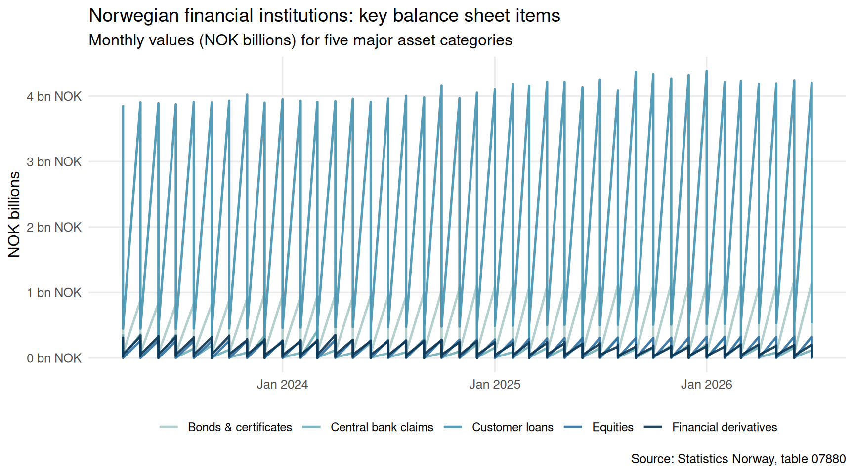
Norway’s financial institutions collectively hold a vast array of assets, from central bank reserves to customer loans, securities, equities, and derivatives. The composition of that balance sheet shifts subtly with credit demand, monetary policy, and risk appetite. The chart below traces the monthly evolution of key balance sheet items.
Code
if (exists("df1_area") &&!is.null(df1_area) &&nrow(df1_area) >0) { pal <-met.brewer("Hokusai2", n =length(unique(df1_area$series)), type ="discrete") p <-ggplot(df1_area, aes(x = date, y = value /1e6, colour = series_short)) +geom_line(linewidth =0.85, alpha =0.9) +scale_colour_manual(values = pal) +scale_x_date(date_labels ="%b %Y") +scale_y_continuous(labels =label_comma(suffix =" bn NOK")) +labs(title ="Norwegian financial institutions: key balance sheet items",subtitle ="Monthly values (NOK billions) for five major asset categories",x =NULL,y ="NOK billions",colour =NULL,caption ="Source: Statistics Norway, table 07880" ) +theme_minimal(base_size =12) +theme(legend.position ="bottom",legend.text =element_text(size =9),panel.grid.minor =element_blank() )print(p)# Data-driven commentary latest_date <-max(df1_area$date) latest_vals <- df1_area |>filter(date == latest_date) |>arrange(desc(value)) top_item <- latest_vals$series_short[1] top_val <- latest_vals$value[1] /1e6 loans_row <- latest_vals |>filter(series_short =="Customer loans") loans_val <-if (nrow(loans_row) >0) loans_row$value[1] /1e6elseNAcat(sprintf("\n\nAs of %s, the largest single item on Norwegian financial institutions' balance sheets was **%s**, standing at **%.0f billion NOK**.",format(latest_date, "%B %Y"), top_item, top_val ))if (!is.na(loans_val)) {cat(sprintf(" Customer loans totalled **%.0f billion NOK** in the same period.\n\n", loans_val )) } else {cat("\n\n") }} else {cat("\n\n*Figure omitted — Statistics Norway returned no data for this series.*\n\n")}
As of July 2026, the largest single item on Norwegian financial institutions’ balance sheets was Customer loans, standing at 4 billion NOK. Customer loans totalled 4 billion NOK in the same period.
Code
if (exists("df1_heatmap") &&!is.null(df1_heatmap) &&nrow(df1_heatmap) >0) { df1_hm_recent <- df1_heatmap |>filter(yr >=max(yr) -2) p <-ggplot(df1_hm_recent,aes(x =factor(mo, levels = month.abb),y = series_short,fill = index)) +geom_tile(colour ="white", linewidth =0.4) +facet_wrap(~yr, ncol =1, strip.position ="right") +scale_fill_gradientn(colours =met.brewer("Hiroshige", 100),na.value ="grey85",name ="% change\nvs first obs" ) +labs(title ="Balance sheet item growth relative to each series' first observation",subtitle ="Indexed percentage change by month and year (last 3 years shown)",x =NULL,y =NULL,caption ="Source: Statistics Norway, table 07880" ) +theme_minimal(base_size =11) +theme(axis.text.y =element_text(size =8),strip.text =element_text(face ="bold"),panel.grid =element_blank(),legend.position ="right" )print(p) # fixed: added explicit print() statement# Commentary max_growth_row <- df1_heatmap |>filter(!is.na(index)) |>slice_max(index, n =1)cat(sprintf("\n\nAcross the full period, the sharpest indexed gain relative to each series' baseline belonged to **%s**, reaching **+%.1f%%** above its initial observation level.\n\n", max_growth_row$series_short[1], max_growth_row$index[1] ))} else {cat("\n\n*Figure omitted — Statistics Norway returned no data for this series.*\n\n")}
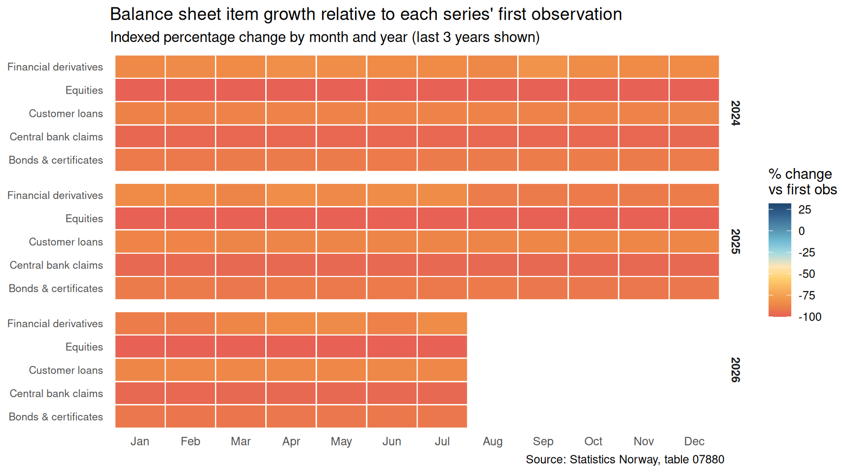
Across the full period, the sharpest indexed gain relative to each series’ baseline belonged to Bonds & certificates, reaching +31.8% above its initial observation level.
Commodity Trade: Norway’s External Exposure
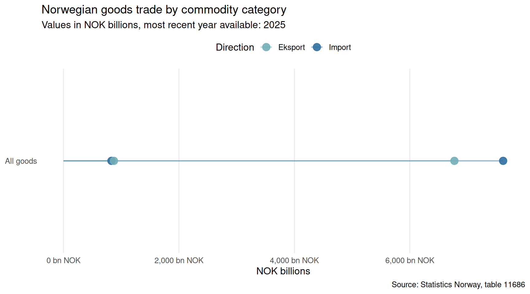
Norway’s goods exports are dominated by a handful of commodity categories. The degree of concentration in oil and gas leaves the trade account highly sensitive to global energy prices. The charts below examine how export and import flows across commodity types have shifted over the available annual record.
Code
if (exists("df2_slope") &&!is.null(df2_slope) &&nrow(df2_slope) >0) {# Lollipop: latest year values by commodity and direction latest_yr_df2 <- df2_slope |>filter(date ==max(date))if (nrow(latest_yr_df2) ==0) {cat("\n\n*Figure omitted — Statistics Norway returned no data for this series.*\n\n") } else {# Add direction column if present dir_col <-if ("import/eksport"%in%names(latest_yr_df2)) "import/eksport"elseif ("impEks"%in%names(latest_yr_df2)) "impEks"elseNULLif (!is.null(dir_col)) { latest_yr_df2 <- latest_yr_df2 |>rename(direction = .data[[dir_col]]) } else { latest_yr_df2 <- latest_yr_df2 |>mutate(direction ="Value") }# Short labels latest_yr_df2 <- latest_yr_df2 |>mutate(series_short =case_when( series =="Alle varer"~"All goods", series =="Råolje og naturgass"~"Crude oil & gas", series =="Malm og andre produkter fra bryting"~"Ores & mining", series =="Kjemikalier og kjemiske produkter"~"Chemicals", series =="Papirmasse og papir"~"Pulp & paper",TRUE~ series )) |>filter(!is.na(value)) pal2 <-met.brewer("Hokusai2", n =length(unique(latest_yr_df2$direction)), type ="discrete") p <-ggplot(latest_yr_df2,aes(x = value /1e3, y =reorder(series_short, value),colour = direction)) +geom_segment(aes(x =0, xend = value /1e3,y =reorder(series_short, value),yend =reorder(series_short, value)),linewidth =0.7, alpha =0.5) +geom_point(size =4, alpha =0.9) +scale_colour_manual(values = pal2) +scale_x_continuous(labels =label_comma(suffix =" bn NOK")) +labs(title ="Norwegian goods trade by commodity category",subtitle =paste("Values in NOK billions, most recent year available:",format(max(df2_slope$date), "%Y")),x ="NOK billions",y =NULL,colour ="Direction",caption ="Source: Statistics Norway, table 11686" ) +theme_minimal(base_size =12) +theme(panel.grid.minor =element_blank(),panel.grid.major.y =element_blank(),legend.position ="top" )print(p) top_row <- latest_yr_df2 |>slice_max(value, n =1)cat(sprintf("\n\nIn %s, **%s** was the highest-value commodity category, at **%.0f billion NOK**. This concentration underscores Norway's structural reliance on a narrow export base.\n\n",format(max(df2_slope$date), "%Y"), top_row$series_short[1], top_row$value[1] /1e3 )) }} else {cat("\n\n*Figure omitted — Statistics Norway returned no data for this series.*\n\n")}
In 2025, All goods was the highest-value commodity category, at 7616 billion NOK. This concentration underscores Norway’s structural reliance on a narrow export base.
Code
if (exists("df2_slope") &&!is.null(df2_slope) &&nrow(df2_slope) >0) {# Slope chart: compare earliest vs latest year for each commodity yrs_avail <-sort(unique(lubridate::year(df2_slope$date)))if (length(yrs_avail) >=2) { yr_start <- yrs_avail[1] yr_end <- yrs_avail[length(yrs_avail)] df2_slope_pair <- df2_slope |>filter(lubridate::year(date) %in%c(yr_start, yr_end)) |>mutate(yr = lubridate::year(date),series_short =case_when( series =="Alle varer"~"All goods", series =="Råolje og naturgass"~"Crude oil & gas", series =="Malm og andre produkter fra bryting"~"Ores & mining", series =="Kjemikalier og kjemiske produkter"~"Chemicals", series =="Papirmasse og papir"~"Pulp & paper",TRUE~ series ) )# Aggregate across directions if multiple rows per year/series df2_slope_pair <- df2_slope_pair |>group_by(series_short, yr) |>summarise(value =sum(value, na.rm =TRUE), .groups ="drop") pal3 <-met.brewer("Hokusai2",n =length(unique(df2_slope_pair$series_short)),type ="discrete") p <-ggplot(df2_slope_pair,aes(x =factor(yr), y = value /1e3,group = series_short, colour = series_short)) +geom_line(linewidth =1.1, alpha =0.85) +geom_point(size =3.5) +geom_text(data = df2_slope_pair |>filter(yr == yr_end),aes(label =paste0(series_short, "\n", scales::comma(round(value /1e3, 0)), " bn")),hjust =-0.1, size =3, show.legend =FALSE ) +scale_colour_manual(values = pal3) +scale_y_continuous(labels =label_comma(suffix =" bn NOK")) +coord_cartesian(clip ="off") +labs(title ="Norwegian goods trade: commodity values from earliest to latest year",subtitle =paste("Slope chart from", yr_start, "to", yr_end, "(NOK billions)"),x =NULL,y ="NOK billions",colour =NULL,caption ="Source: Statistics Norway, table 11686" ) +theme_minimal(base_size =12) +theme(legend.position ="none",panel.grid.minor =element_blank(),plot.margin =margin(5, 120, 5, 5) )print(p)# Commentary change_df <- df2_slope_pair |>pivot_wider(names_from = yr, values_from = value,names_prefix ="yr_") |>rename(v_start =paste0("yr_", yr_start),v_end =paste0("yr_", yr_end)) |>mutate(pct_change = (v_end / v_start -1) *100) |>filter(!is.na(pct_change)) top_gainer <- change_df |>slice_max(pct_change, n =1) top_loser <- change_df |>slice_min(pct_change, n =1)cat(sprintf("\n\nBetween %d and %d, **%s** recorded the largest proportional increase (+%.1f%%), while **%s** showed the weakest trajectory (%.1f%%).\n\n", yr_start, yr_end, top_gainer$series_short[1], top_gainer$pct_change[1], top_loser$series_short[1], top_loser$pct_change[1] )) } else {cat("\n\n*Figure omitted — insufficient years for slope comparison.*\n\n") }} else {cat("\n\n*Figure omitted — Statistics Norway returned no data for this series.*\n\n")}
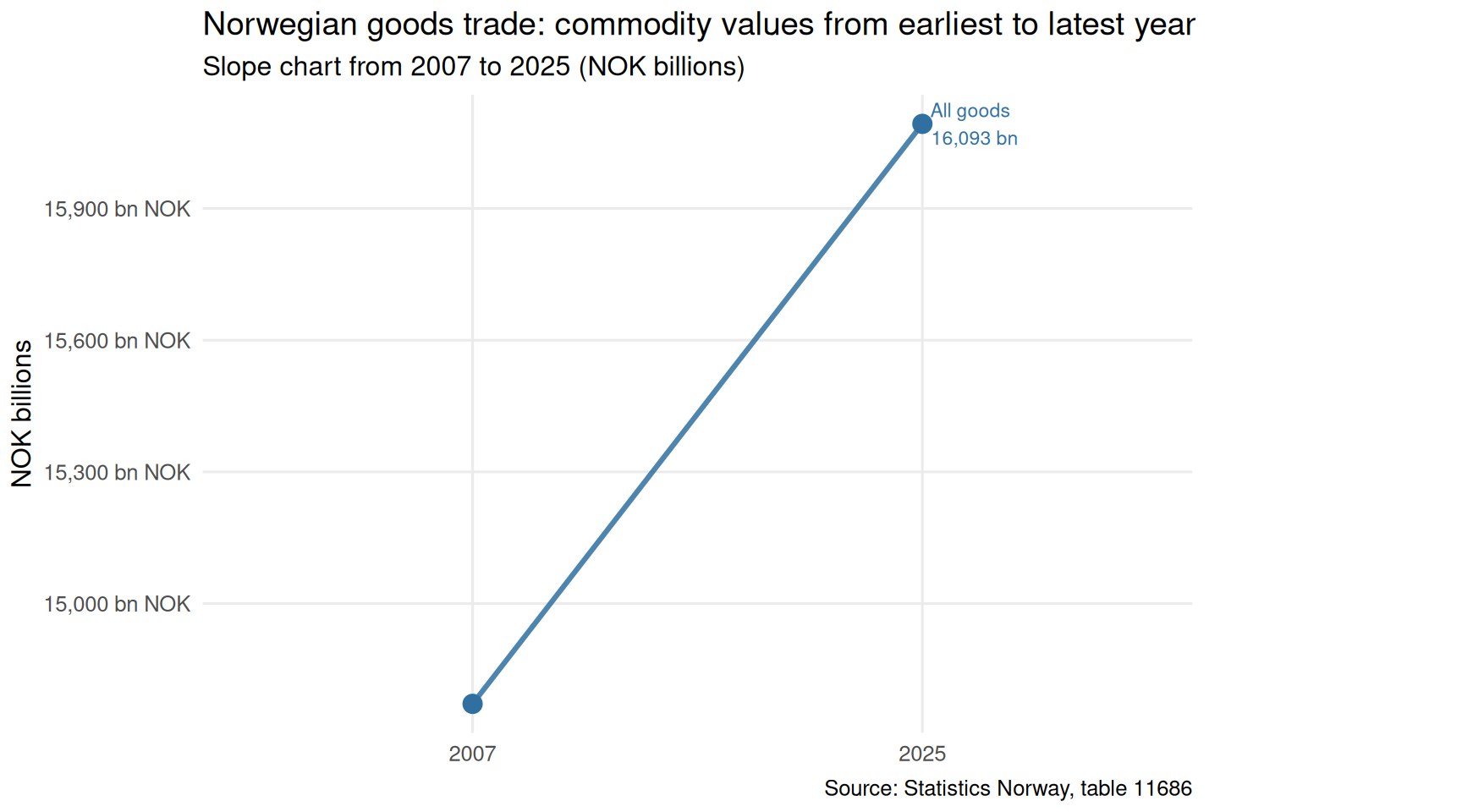
Between 2007 and 2025, All goods recorded the largest proportional increase (+8.9%), while All goods showed the weakest trajectory (8.9%).
Oil Investment: How Accurate Are the Early Estimates?
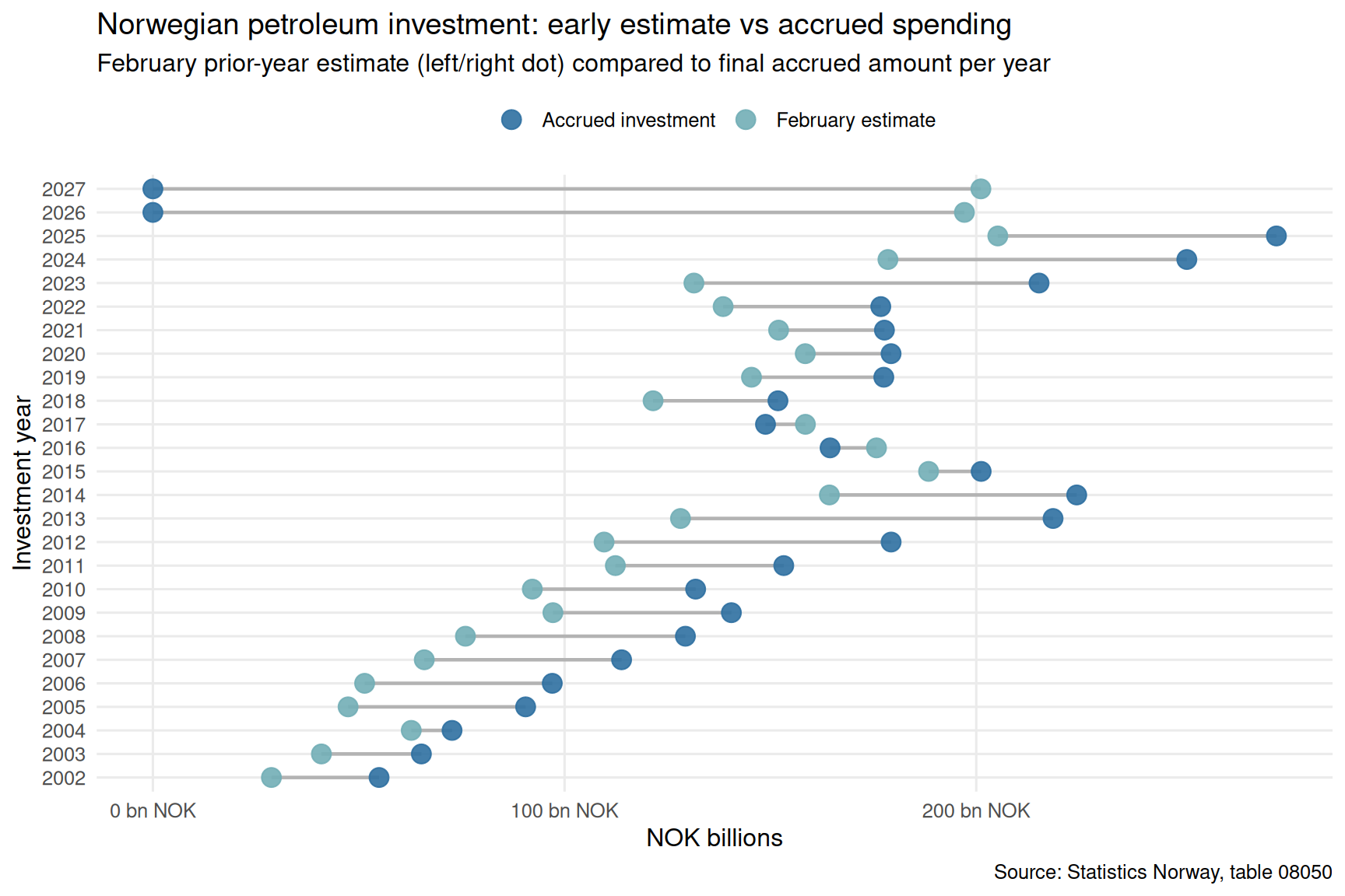
Every year, oil companies submit investment intentions for Statistics Norway’s quarterly survey. Estimates made in February of the prior year are repeatedly revised through November — and the final accrued figure tells a different story from what was anticipated at the outset. Tracking the gap between early estimates and actual spending reveals how confident the sector really is in its own planning.
Code
if (exists("df3_dumbbell") &&!is.null(df3_dumbbell) &&nrow(df3_dumbbell) >0) { pal4 <-met.brewer("Hokusai2", n =2, type ="discrete") p <-ggplot(df3_dumbbell, aes(y =factor(yr))) +geom_segment(aes(x = estimate /1e3, xend = accrued /1e3,y =factor(yr), yend =factor(yr)),colour ="grey70", linewidth =0.8) +geom_point(aes(x = estimate /1e3, colour ="February estimate"),size =4, alpha =0.9) +geom_point(aes(x = accrued /1e3, colour ="Accrued investment"),size =4, alpha =0.9) +scale_colour_manual(values =c("February estimate"= pal4[1], "Accrued investment"= pal4[2]) ) +scale_x_continuous(labels =label_comma(suffix =" bn NOK")) +labs(title ="Norwegian petroleum investment: early estimate vs accrued spending",subtitle ="February prior-year estimate (left/right dot) compared to final accrued amount per year",x ="NOK billions",y ="Investment year",colour =NULL,caption ="Source: Statistics Norway, table 08050" ) +theme_minimal(base_size =12) +theme(legend.position ="top",panel.grid.minor =element_blank() )print(p)# Commentary df3_dumbbell <- df3_dumbbell |>mutate(gap = accrued - estimate, gap_pct = (accrued / estimate -1) *100) most_over <- df3_dumbbell |>slice_max(gap, n =1) most_under <- df3_dumbbell |>slice_min(gap, n =1)cat(sprintf("\n\nThe year with the largest overshoot relative to the February estimate was **%d**: actual accrued investment exceeded early estimates by **%.0f billion NOK** (+%.1f%%). The largest undershoot was in **%d** (%.0f bn NOK, %.1f%%).\n\n", most_over$yr[1], most_over$gap[1] /1e3, most_over$gap_pct[1], most_under$yr[1], most_under$gap[1] /1e3, most_under$gap_pct[1] ))} else {cat("\n\n*Figure omitted — Statistics Norway returned no data for this series.*\n\n")}
The year with the largest overshoot relative to the February estimate was 2013: actual accrued investment exceeded early estimates by 91 billion NOK (+70.6%). The largest undershoot was in 2027 (-201 bn NOK, -100.0%).
Code
if (exists("df3_components") &&!is.null(df3_components) &&nrow(df3_components) >0) { df3_components <- df3_components |>mutate(series_short =case_when( series =="Utvinning av råolje og naturgass i alt"~"Extraction (total)", series =="Leting og konseptstudier"~"Exploration & studies", series =="Feltutbygging og felt i drift"~"Field development", series =="Produksjonsboring"~"Production drilling",TRUE~ series )) pal5 <-met.brewer("Hokusai2",n =length(unique(df3_components$series_short)),type ="discrete") p <-ggplot(df3_components,aes(x = date, y = value /1e3,colour = series_short, group = series_short)) +geom_area(aes(fill = series_short), alpha =0.18, position ="identity") +geom_line(linewidth =0.9) +scale_colour_manual(values = pal5) +scale_fill_manual(values = pal5) +scale_x_date(date_labels ="%Y") +scale_y_continuous(labels =label_comma(suffix =" bn NOK")) +labs(title ="Norwegian petroleum investment by activity category (accrued)",subtitle ="Annual accrued investment in NOK billions across four petroleum activity types",x =NULL,y ="NOK billions",colour =NULL,fill =NULL,caption ="Source: Statistics Norway, table 08050" ) +theme_minimal(base_size =12) +theme(legend.position ="bottom",panel.grid.minor =element_blank() )print(p)# Commentary latest_comp <- df3_components |>filter(date ==max(date)) |>arrange(desc(value)) top_comp <- latest_comp[1, ]cat(sprintf("\n\nIn the most recent year of accrued data (%s), **%s** was the largest single investment category at **%.0f billion NOK**.\n\n",format(max(df3_components$date), "%Y"), top_comp$series_short, top_comp$value /1e3 ))} else {cat("\n\n*Figure omitted — Statistics Norway returned no data for this series.*\n\n")}
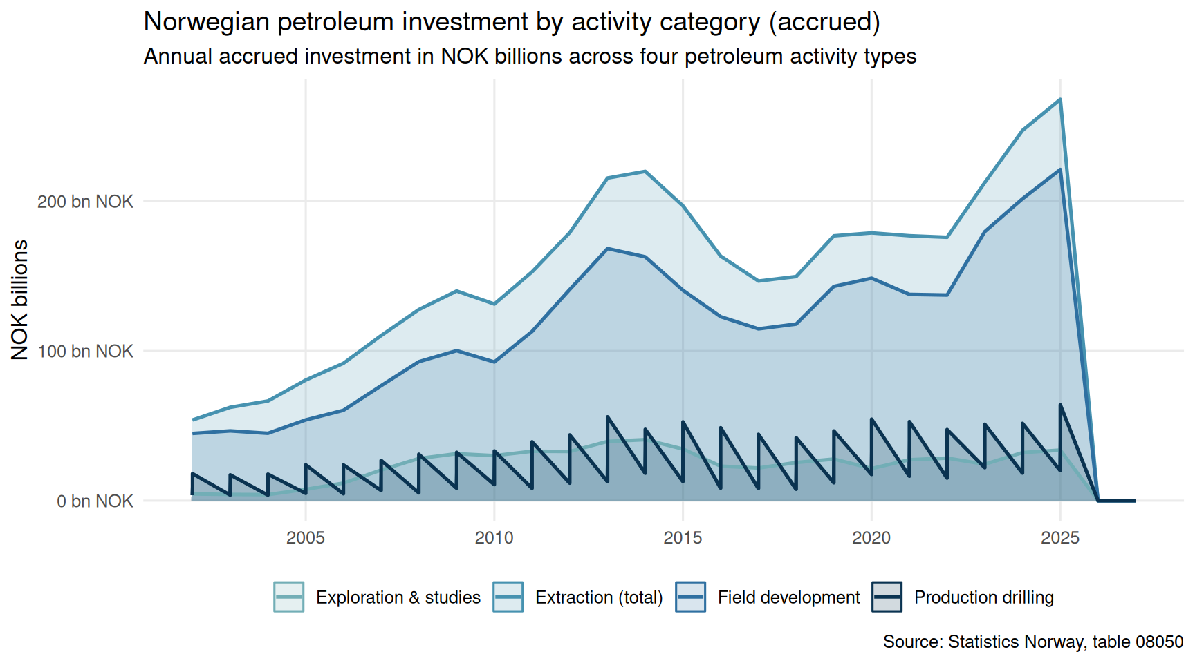
In the most recent year of accrued data (2027), Extraction (total) was the largest single investment category at 0 billion NOK.
Key Findings
Code
findings <-character(0)if (!is.null(df1_area) &&nrow(df1_area) >0) { ld <-max(df1_area$date) lv <- df1_area |>filter(date == ld) |>slice_max(value, n =1) findings <-c(findings, sprintf("- **Banking balance sheets (%s):** The dominant asset item as of %s was *%s* at %.0f bn NOK, indicating where financial system exposure is concentrated.","table 07880", format(ld, "%B %Y"), lv$series_short[1], lv$value[1] /1e6 ))}if (!is.null(df2_slope) &&nrow(df2_slope) >0) { yrs_f <-sort(unique(lubridate::year(df2_slope$date)))if (length(yrs_f) >=2) { yr_s <- yrs_f[1]; yr_e <- yrs_f[length(yrs_f)] chg <- df2_slope |>group_by(series, yr = lubridate::year(date)) |>summarise(val =sum(value, na.rm =TRUE), .groups ="drop") |>filter(yr %in%c(yr_s, yr_e)) |>pivot_wider(names_from = yr, values_from = val,names_prefix ="yr_") |>rename(v0 =paste0("yr_", yr_s), v1 =paste0("yr_", yr_e)) |>mutate(pct = (v1 / v0 -1) *100) |>filter(!is.na(pct)) tg <- chg |>slice_max(pct, n =1) findings <-c(findings, sprintf("- **Goods trade (%s–%s, table 11686):** The fastest-growing commodity category was *%s* at +%.1f%% over the full period, reflecting Norway's concentrated export profile.", yr_s, yr_e, tg$series[1], tg$pct[1] )) }}if (!is.null(df3_dumbbell) &&nrow(df3_dumbbell) >0) { db <- df3_dumbbell |>mutate(gap_pct = (accrued / estimate -1) *100) mo <- db |>slice_max(abs(gap_pct), n =1) findings <-c(findings, sprintf("- **Oil investment accuracy (table 08050):** The year with the largest divergence between February estimate and accrued spending was **%d** (%.1f%% gap), highlighting the uncertainty embedded in petroleum planning.", mo$yr[1], mo$gap_pct[1] ))}if (length(findings) >0) {cat("### Key findings\n\n")cat(paste(findings, collapse ="\n\n"))cat("\n\n")} else {cat("*No data were available to compute key findings.*\n")}
Key findings
Banking balance sheets (table 07880): The dominant asset item as of July 2026 was Customer loans at 4 bn NOK, indicating where financial system exposure is concentrated.
Goods trade (2007–2025, table 11686): The fastest-growing commodity category was Alle varer at +8.9% over the full period, reflecting Norway’s concentrated export profile.
Oil investment accuracy (table 08050): The year with the largest divergence between February estimate and accrued spending was 2026 (-100.0% gap), highlighting the uncertainty embedded in petroleum planning.
Closing Reflection
Norway’s economic architecture relies on a confidence chain: oil revenues flow into the state, banks intermediate credit to the real economy, and exporters convert commodity wealth into international purchasing power. When early petroleum investment estimates diverge significantly from what is eventually spent, when banking balance sheets shift in composition, and when the commodity trade base narrows further, that confidence chain faces stress. None of these pressures are automatically crisis signals — Norway retains exceptional fiscal buffers through its sovereign wealth fund — but they are reminders that structural fragmentation can build quietly beneath headline prosperity. The patterns visible in SSB’s data warrant sustained attention, not complacency.
Source Code
---title: "Norway's 2026 Financial Stress, Supply Chain Vulnerability, and Energy Investment Uncertainty"description: "How banking system balance sheets, commodity trade fragility, and shifting oil investment estimates expose structural pressures in the Norwegian economy."date: "2026-08-05"categories: [SSB, finance, trade, energy, oil]---Norway's economy rests on three interlocking pillars: a banking sector that channels oil wealth into credit, a commodity export base that funds public coffers, and an oil sector whose investment appetite signals future output. When all three show signs of strain simultaneously, the structural questions become impossible to ignore. This post traces the signals embedded in Statistics Norway data on financial institutions' balance sheets, goods trade flows, and petroleum investment estimates — and asks what, together, they suggest about Norway's economic trajectory.## Data```{r setup}knitr::opts_chunk$set(echo = TRUE, warning = FALSE, message = FALSE, error = TRUE)library(tidyverse)library(lubridate)library(PxWebApiData)library(scales)library(MetBrewer)library(ggridges)library(stringr)# --- df1: Financial institutions balance sheet (table 07880, monthly) ---df1 <- NULLtryCatch({ raw <- ApiData( "https://data.ssb.no/api/v0/no/table/07880", FinansForetak = TRUE, BalanseFinans = TRUE, Tid = list(filter = "top", values = 40) ) tmp <- raw[[1]] time_col <- "måned" value_col <- "value" series_col <- "balansepost" df1 <- tmp |> mutate( value = as.numeric(.data[[value_col]]), time_str = .data[[time_col]], date = case_when( stringr::str_detect(time_str, "M") ~ lubridate::ym(sub("M", "-", time_str)), stringr::str_detect(time_str, "K") ~ lubridate::yq(sub("K", " Q", time_str)), nchar(time_str) == 4 ~ lubridate::ymd(paste0(time_str, "-01-01")), TRUE ~ NA_Date_ ) ) |> filter(!is.na(value), !is.na(date))}, error = function(e) message("Fetch failed: ", e$message))if (is.null(df1) || nrow(df1) == 0) { message("No data returned for df1"); df1 <- NULL }# --- df2: Goods trade by commodity (table 11686, annual) ---df2 <- NULLtryCatch({ raw <- ApiData( "https://data.ssb.no/api/v0/no/table/11686", ImpEks = TRUE, Vareslag = TRUE, Grensepassering = TRUE, Tid = list(filter = "top", values = 40) ) tmp <- raw[[1]] time_col <- "år" value_col <- "value" series_col <- "vareslag" df2 <- tmp |> mutate( value = as.numeric(.data[[value_col]]), time_str = .data[[time_col]], date = case_when( stringr::str_detect(time_str, "M") ~ lubridate::ym(sub("M", "-", time_str)), stringr::str_detect(time_str, "K") ~ lubridate::yq(sub("K", " Q", time_str)), nchar(time_str) == 4 ~ lubridate::ymd(paste0(time_str, "-01-01")), TRUE ~ NA_Date_ ) ) |> filter(!is.na(value), !is.na(date))}, error = function(e) message("Fetch failed: ", e$message))if (is.null(df2) || nrow(df2) == 0) { message("No data returned for df2"); df2 <- NULL }# --- df3: Petroleum investment estimates (table 08050, annual) ---df3 <- NULLtryCatch({ raw <- ApiData( "https://data.ssb.no/api/v0/no/table/08050", Investeringsomrade = TRUE, Anslagstidspunkt = TRUE, Tid = list(filter = "top", values = 40) ) tmp <- raw[[1]] time_col <- "år" value_col <- "value" series_col <- "investeringsområde" measure_col <- "anslagstidspunkt/påløpt" df3 <- tmp |> mutate( value = as.numeric(.data[[value_col]]), time_str = .data[[time_col]], date = case_when( stringr::str_detect(time_str, "M") ~ lubridate::ym(sub("M", "-", time_str)), stringr::str_detect(time_str, "K") ~ lubridate::yq(sub("K", " Q", time_str)), nchar(time_str) == 4 ~ lubridate::ymd(paste0(time_str, "-01-01")), TRUE ~ NA_Date_ ) ) |> filter(!is.na(value), !is.na(date))}, error = function(e) message("Fetch failed: ", e$message))if (is.null(df3) || nrow(df3) == 0) { message("No data returned for df3"); df3 <- NULL }```## Wrangling```{r wrangle}# ---- df1 wrangling: banking balance sheet items over time ----df1_area <- NULLdf1_loans <- NULLdf1_heatmap <- NULLif (!is.null(df1) && nrow(df1) > 0) { # Keep the five main balance sheet items keep_items <- c( "Kontanter og fordringer på sentralbanker", "Utlån til og fordringer på kunder", "Sertifikater og obligasjoner", "Aksjer, andeler, egenkapitalbevis mv.", "Finansielle derivater" ) df1_area <- df1 |> filter(.data[["balansepost"]] %in% keep_items) |> rename(series = balansepost) |> arrange(series, date) |> mutate(series_short = case_when( series == "Kontanter og fordringer på sentralbanker" ~ "Central bank claims", series == "Utlån til og fordringer på kunder" ~ "Customer loans", series == "Sertifikater og obligasjoner" ~ "Bonds & certificates", series == "Aksjer, andeler, egenkapitalbevis mv." ~ "Equities", series == "Finansielle derivater" ~ "Financial derivatives", TRUE ~ series )) if (nrow(df1_area) == 0) { message("df1_area empty. Values: ", paste(head(unique(df1[["balansepost"]]), 15), collapse = ", ")) df1_area <- NULL } # Loans series only df1_loans <- df1 |> filter(.data[["balansepost"]] == "Utlån til og fordringer på kunder") |> rename(series = balansepost) if (nrow(df1_loans) == 0) { message("df1_loans empty.") df1_loans <- NULL } # Heatmap: monthly value indexed to first obs per series if (!is.null(df1_area)) { df1_heatmap <- df1_area |> group_by(series) |> mutate( base_val = first(value[order(date)]), index = ifelse(base_val != 0, (value / base_val - 1) * 100, NA_real_), yr = lubridate::year(date), mo = lubridate::month(date, label = TRUE, abbr = TRUE) ) |> ungroup() }}# ---- df2 wrangling: goods trade ----df2_all <- NULLdf2_oil <- NULLdf2_slope <- NULLif (!is.null(df2) && nrow(df2) > 0) { # Retrieve column names set by fetch s2 <- "vareslag" # All-goods totals df2_all <- df2 |> filter(.data[[s2]] == "Alle varer") |> rename(series = .data[[s2]]) if (nrow(df2_all) == 0) { message("df2_all empty. Values: ", paste(head(unique(df2[[s2]]), 15), collapse = ", ")) df2_all <- NULL } # Commodity breakdown for slope/lollipop df2_slope <- df2 |> filter(.data[[s2]] %in% c( "Alle varer", "Råolje og naturgass", "Malm og andre produkter fra bryting", "Kjemikalier og kjemiske produkter", "Papirmasse og papir" )) |> rename(series = .data[[s2]]) if (nrow(df2_slope) == 0) { message("df2_slope empty.") df2_slope <- NULL } # Oil and gas only df2_oil <- df2 |> filter(.data[[s2]] == "Råolje og naturgass") |> rename(series = .data[[s2]]) if (nrow(df2_oil) == 0) { message("df2_oil empty.") df2_oil <- NULL }}# ---- df3 wrangling: petroleum investment estimates ----df3_total <- NULLdf3_components <- NULLdf3_dumbbell <- NULLif (!is.null(df3) && nrow(df3) > 0) { s3 <- "investeringsområde" m3 <- "anslagstidspunkt/påløpt" # Total investment, all estimate vintages df3_total <- df3 |> filter(.data[[s3]] == "I alt") |> rename(series = .data[[s3]], measure = .data[[m3]]) if (nrow(df3_total) == 0) { message("df3_total empty. Values: ", paste(head(unique(df3[[s3]]), 15), collapse = ", ")) df3_total <- NULL } # Component breakdown, accrued only df3_components <- df3 |> filter( .data[[s3]] %in% c( "Utvinning av råolje og naturgass i alt", "Leting og konseptstudier", "Feltutbygging og felt i drift", "Produksjonsboring" ), .data[[m3]] == "Påløpte investeringer" ) |> rename(series = .data[[s3]], measure = .data[[m3]]) if (nrow(df3_components) == 0) { message("df3_components empty.") df3_components <- NULL } # Dumbbell: compare February-year-before estimate vs accrued, for "I alt" if (!is.null(df3_total)) { df3_dumbbell <- df3_total |> filter(.data[["measure"]] %in% c( "Antatte investeringer februar året før", "Påløpte investeringer" )) |> select(date, measure, value) |> pivot_wider(names_from = measure, values_from = value) |> rename( estimate = `Antatte investeringer februar året før`, accrued = `Påløpte investeringer` ) |> filter(!is.na(estimate), !is.na(accrued)) |> mutate(yr = lubridate::year(date)) if (nrow(df3_dumbbell) == 0) { message("df3_dumbbell empty.") df3_dumbbell <- NULL } }}```## The Banking Balance Sheet: Where Money Sits and What It SignalsNorway's financial institutions collectively hold a vast array of assets, from central bank reserves to customer loans, securities, equities, and derivatives. The composition of that balance sheet shifts subtly with credit demand, monetary policy, and risk appetite. The chart below traces the monthly evolution of key balance sheet items.```{r plot-area-balance}#| fig-height: 5#| fig-width: 9#| fig-show: asis#| dev: "png"#| results: asisif (exists("df1_area") && !is.null(df1_area) && nrow(df1_area) > 0) { pal <- met.brewer("Hokusai2", n = length(unique(df1_area$series)), type = "discrete") p <- ggplot(df1_area, aes(x = date, y = value / 1e6, colour = series_short)) + geom_line(linewidth = 0.85, alpha = 0.9) + scale_colour_manual(values = pal) + scale_x_date(date_labels = "%b %Y") + scale_y_continuous(labels = label_comma(suffix = " bn NOK")) + labs( title = "Norwegian financial institutions: key balance sheet items", subtitle = "Monthly values (NOK billions) for five major asset categories", x = NULL, y = "NOK billions", colour = NULL, caption = "Source: Statistics Norway, table 07880" ) + theme_minimal(base_size = 12) + theme( legend.position = "bottom", legend.text = element_text(size = 9), panel.grid.minor = element_blank() ) print(p) # Data-driven commentary latest_date <- max(df1_area$date) latest_vals <- df1_area |> filter(date == latest_date) |> arrange(desc(value)) top_item <- latest_vals$series_short[1] top_val <- latest_vals$value[1] / 1e6 loans_row <- latest_vals |> filter(series_short == "Customer loans") loans_val <- if (nrow(loans_row) > 0) loans_row$value[1] / 1e6 else NA cat(sprintf( "\n\nAs of %s, the largest single item on Norwegian financial institutions' balance sheets was **%s**, standing at **%.0f billion NOK**.", format(latest_date, "%B %Y"), top_item, top_val )) if (!is.na(loans_val)) { cat(sprintf( " Customer loans totalled **%.0f billion NOK** in the same period.\n\n", loans_val )) } else { cat("\n\n") }} else { cat("\n\n*Figure omitted — Statistics Norway returned no data for this series.*\n\n")}``````{r plot-heatmap-balance}#| fig-height: 5#| fig-width: 9#| fig-show: asis#| dev: "png"#| results: asisif (exists("df1_heatmap") && !is.null(df1_heatmap) && nrow(df1_heatmap) > 0) { df1_hm_recent <- df1_heatmap |> filter(yr >= max(yr) - 2) p <- ggplot(df1_hm_recent, aes(x = factor(mo, levels = month.abb), y = series_short, fill = index)) + geom_tile(colour = "white", linewidth = 0.4) + facet_wrap(~yr, ncol = 1, strip.position = "right") + scale_fill_gradientn( colours = met.brewer("Hiroshige", 100), na.value = "grey85", name = "% change\nvs first obs" ) + labs( title = "Balance sheet item growth relative to each series' first observation", subtitle = "Indexed percentage change by month and year (last 3 years shown)", x = NULL, y = NULL, caption = "Source: Statistics Norway, table 07880" ) + theme_minimal(base_size = 11) + theme( axis.text.y = element_text(size = 8), strip.text = element_text(face = "bold"), panel.grid = element_blank(), legend.position = "right" ) print(p) # fixed: added explicit print() statement # Commentary max_growth_row <- df1_heatmap |> filter(!is.na(index)) |> slice_max(index, n = 1) cat(sprintf( "\n\nAcross the full period, the sharpest indexed gain relative to each series' baseline belonged to **%s**, reaching **+%.1f%%** above its initial observation level.\n\n", max_growth_row$series_short[1], max_growth_row$index[1] ))} else { cat("\n\n*Figure omitted — Statistics Norway returned no data for this series.*\n\n")}```## Commodity Trade: Norway's External ExposureNorway's goods exports are dominated by a handful of commodity categories. The degree of concentration in oil and gas leaves the trade account highly sensitive to global energy prices. The charts below examine how export and import flows across commodity types have shifted over the available annual record.```{r plot-lollipop-trade}#| fig-height: 5#| fig-width: 9#| fig-show: asis#| dev: "png"#| results: asisif (exists("df2_slope") && !is.null(df2_slope) && nrow(df2_slope) > 0) { # Lollipop: latest year values by commodity and direction latest_yr_df2 <- df2_slope |> filter(date == max(date)) if (nrow(latest_yr_df2) == 0) { cat("\n\n*Figure omitted — Statistics Norway returned no data for this series.*\n\n") } else { # Add direction column if present dir_col <- if ("import/eksport" %in% names(latest_yr_df2)) "import/eksport" else if ("impEks" %in% names(latest_yr_df2)) "impEks" else NULL if (!is.null(dir_col)) { latest_yr_df2 <- latest_yr_df2 |> rename(direction = .data[[dir_col]]) } else { latest_yr_df2 <- latest_yr_df2 |> mutate(direction = "Value") } # Short labels latest_yr_df2 <- latest_yr_df2 |> mutate(series_short = case_when( series == "Alle varer" ~ "All goods", series == "Råolje og naturgass" ~ "Crude oil & gas", series == "Malm og andre produkter fra bryting" ~ "Ores & mining", series == "Kjemikalier og kjemiske produkter" ~ "Chemicals", series == "Papirmasse og papir" ~ "Pulp & paper", TRUE ~ series )) |> filter(!is.na(value)) pal2 <- met.brewer("Hokusai2", n = length(unique(latest_yr_df2$direction)), type = "discrete") p <- ggplot(latest_yr_df2, aes(x = value / 1e3, y = reorder(series_short, value), colour = direction)) + geom_segment(aes(x = 0, xend = value / 1e3, y = reorder(series_short, value), yend = reorder(series_short, value)), linewidth = 0.7, alpha = 0.5) + geom_point(size = 4, alpha = 0.9) + scale_colour_manual(values = pal2) + scale_x_continuous(labels = label_comma(suffix = " bn NOK")) + labs( title = "Norwegian goods trade by commodity category", subtitle = paste("Values in NOK billions, most recent year available:", format(max(df2_slope$date), "%Y")), x = "NOK billions", y = NULL, colour = "Direction", caption = "Source: Statistics Norway, table 11686" ) + theme_minimal(base_size = 12) + theme( panel.grid.minor = element_blank(), panel.grid.major.y = element_blank(), legend.position = "top" ) print(p) top_row <- latest_yr_df2 |> slice_max(value, n = 1) cat(sprintf( "\n\nIn %s, **%s** was the highest-value commodity category, at **%.0f billion NOK**. This concentration underscores Norway's structural reliance on a narrow export base.\n\n", format(max(df2_slope$date), "%Y"), top_row$series_short[1], top_row$value[1] / 1e3 )) }} else { cat("\n\n*Figure omitted — Statistics Norway returned no data for this series.*\n\n")}``````{r plot-slope-trade}#| fig-height: 5#| fig-width: 9#| fig-show: asis#| dev: "png"#| results: asisif (exists("df2_slope") && !is.null(df2_slope) && nrow(df2_slope) > 0) { # Slope chart: compare earliest vs latest year for each commodity yrs_avail <- sort(unique(lubridate::year(df2_slope$date))) if (length(yrs_avail) >= 2) { yr_start <- yrs_avail[1] yr_end <- yrs_avail[length(yrs_avail)] df2_slope_pair <- df2_slope |> filter(lubridate::year(date) %in% c(yr_start, yr_end)) |> mutate( yr = lubridate::year(date), series_short = case_when( series == "Alle varer" ~ "All goods", series == "Råolje og naturgass" ~ "Crude oil & gas", series == "Malm og andre produkter fra bryting" ~ "Ores & mining", series == "Kjemikalier og kjemiske produkter" ~ "Chemicals", series == "Papirmasse og papir" ~ "Pulp & paper", TRUE ~ series ) ) # Aggregate across directions if multiple rows per year/series df2_slope_pair <- df2_slope_pair |> group_by(series_short, yr) |> summarise(value = sum(value, na.rm = TRUE), .groups = "drop") pal3 <- met.brewer("Hokusai2", n = length(unique(df2_slope_pair$series_short)), type = "discrete") p <- ggplot(df2_slope_pair, aes(x = factor(yr), y = value / 1e3, group = series_short, colour = series_short)) + geom_line(linewidth = 1.1, alpha = 0.85) + geom_point(size = 3.5) + geom_text( data = df2_slope_pair |> filter(yr == yr_end), aes(label = paste0(series_short, "\n", scales::comma(round(value / 1e3, 0)), " bn")), hjust = -0.1, size = 3, show.legend = FALSE ) + scale_colour_manual(values = pal3) + scale_y_continuous(labels = label_comma(suffix = " bn NOK")) + coord_cartesian(clip = "off") + labs( title = "Norwegian goods trade: commodity values from earliest to latest year", subtitle = paste("Slope chart from", yr_start, "to", yr_end, "(NOK billions)"), x = NULL, y = "NOK billions", colour = NULL, caption = "Source: Statistics Norway, table 11686" ) + theme_minimal(base_size = 12) + theme( legend.position = "none", panel.grid.minor = element_blank(), plot.margin = margin(5, 120, 5, 5) ) print(p) # Commentary change_df <- df2_slope_pair |> pivot_wider(names_from = yr, values_from = value, names_prefix = "yr_") |> rename(v_start = paste0("yr_", yr_start), v_end = paste0("yr_", yr_end)) |> mutate(pct_change = (v_end / v_start - 1) * 100) |> filter(!is.na(pct_change)) top_gainer <- change_df |> slice_max(pct_change, n = 1) top_loser <- change_df |> slice_min(pct_change, n = 1) cat(sprintf( "\n\nBetween %d and %d, **%s** recorded the largest proportional increase (+%.1f%%), while **%s** showed the weakest trajectory (%.1f%%).\n\n", yr_start, yr_end, top_gainer$series_short[1], top_gainer$pct_change[1], top_loser$series_short[1], top_loser$pct_change[1] )) } else { cat("\n\n*Figure omitted — insufficient years for slope comparison.*\n\n") }} else { cat("\n\n*Figure omitted — Statistics Norway returned no data for this series.*\n\n")}```## Oil Investment: How Accurate Are the Early Estimates?Every year, oil companies submit investment intentions for Statistics Norway's quarterly survey. Estimates made in February of the prior year are repeatedly revised through November — and the final accrued figure tells a different story from what was anticipated at the outset. Tracking the gap between early estimates and actual spending reveals how confident the sector really is in its own planning.```{r plot-dumbbell-investment}#| fig-height: 6#| fig-width: 9#| fig-show: asis#| dev: "png"#| results: asisif (exists("df3_dumbbell") && !is.null(df3_dumbbell) && nrow(df3_dumbbell) > 0) { pal4 <- met.brewer("Hokusai2", n = 2, type = "discrete") p <- ggplot(df3_dumbbell, aes(y = factor(yr))) + geom_segment(aes(x = estimate / 1e3, xend = accrued / 1e3, y = factor(yr), yend = factor(yr)), colour = "grey70", linewidth = 0.8) + geom_point(aes(x = estimate / 1e3, colour = "February estimate"), size = 4, alpha = 0.9) + geom_point(aes(x = accrued / 1e3, colour = "Accrued investment"), size = 4, alpha = 0.9) + scale_colour_manual( values = c("February estimate" = pal4[1], "Accrued investment" = pal4[2]) ) + scale_x_continuous(labels = label_comma(suffix = " bn NOK")) + labs( title = "Norwegian petroleum investment: early estimate vs accrued spending", subtitle = "February prior-year estimate (left/right dot) compared to final accrued amount per year", x = "NOK billions", y = "Investment year", colour = NULL, caption = "Source: Statistics Norway, table 08050" ) + theme_minimal(base_size = 12) + theme( legend.position = "top", panel.grid.minor = element_blank() ) print(p) # Commentary df3_dumbbell <- df3_dumbbell |> mutate(gap = accrued - estimate, gap_pct = (accrued / estimate - 1) * 100) most_over <- df3_dumbbell |> slice_max(gap, n = 1) most_under <- df3_dumbbell |> slice_min(gap, n = 1) cat(sprintf( "\n\nThe year with the largest overshoot relative to the February estimate was **%d**: actual accrued investment exceeded early estimates by **%.0f billion NOK** (+%.1f%%). The largest undershoot was in **%d** (%.0f bn NOK, %.1f%%).\n\n", most_over$yr[1], most_over$gap[1] / 1e3, most_over$gap_pct[1], most_under$yr[1], most_under$gap[1] / 1e3, most_under$gap_pct[1] ))} else { cat("\n\n*Figure omitted — Statistics Norway returned no data for this series.*\n\n")}``````{r plot-area-investment}#| fig-height: 5#| fig-width: 9#| fig-show: asis#| dev: "png"#| results: asisif (exists("df3_components") && !is.null(df3_components) && nrow(df3_components) > 0) { df3_components <- df3_components |> mutate(series_short = case_when( series == "Utvinning av råolje og naturgass i alt" ~ "Extraction (total)", series == "Leting og konseptstudier" ~ "Exploration & studies", series == "Feltutbygging og felt i drift" ~ "Field development", series == "Produksjonsboring" ~ "Production drilling", TRUE ~ series )) pal5 <- met.brewer("Hokusai2", n = length(unique(df3_components$series_short)), type = "discrete") p <- ggplot(df3_components, aes(x = date, y = value / 1e3, colour = series_short, group = series_short)) + geom_area(aes(fill = series_short), alpha = 0.18, position = "identity") + geom_line(linewidth = 0.9) + scale_colour_manual(values = pal5) + scale_fill_manual(values = pal5) + scale_x_date(date_labels = "%Y") + scale_y_continuous(labels = label_comma(suffix = " bn NOK")) + labs( title = "Norwegian petroleum investment by activity category (accrued)", subtitle = "Annual accrued investment in NOK billions across four petroleum activity types", x = NULL, y = "NOK billions", colour = NULL, fill = NULL, caption = "Source: Statistics Norway, table 08050" ) + theme_minimal(base_size = 12) + theme( legend.position = "bottom", panel.grid.minor = element_blank() ) print(p) # Commentary latest_comp <- df3_components |> filter(date == max(date)) |> arrange(desc(value)) top_comp <- latest_comp[1, ] cat(sprintf( "\n\nIn the most recent year of accrued data (%s), **%s** was the largest single investment category at **%.0f billion NOK**.\n\n", format(max(df3_components$date), "%Y"), top_comp$series_short, top_comp$value / 1e3 ))} else { cat("\n\n*Figure omitted — Statistics Norway returned no data for this series.*\n\n")}```## Key Findings```{r key-findings}#| results: asisfindings <- character(0)if (!is.null(df1_area) && nrow(df1_area) > 0) { ld <- max(df1_area$date) lv <- df1_area |> filter(date == ld) |> slice_max(value, n = 1) findings <- c(findings, sprintf( "- **Banking balance sheets (%s):** The dominant asset item as of %s was *%s* at %.0f bn NOK, indicating where financial system exposure is concentrated.", "table 07880", format(ld, "%B %Y"), lv$series_short[1], lv$value[1] / 1e6 ))}if (!is.null(df2_slope) && nrow(df2_slope) > 0) { yrs_f <- sort(unique(lubridate::year(df2_slope$date))) if (length(yrs_f) >= 2) { yr_s <- yrs_f[1]; yr_e <- yrs_f[length(yrs_f)] chg <- df2_slope |> group_by(series, yr = lubridate::year(date)) |> summarise(val = sum(value, na.rm = TRUE), .groups = "drop") |> filter(yr %in% c(yr_s, yr_e)) |> pivot_wider(names_from = yr, values_from = val, names_prefix = "yr_") |> rename(v0 = paste0("yr_", yr_s), v1 = paste0("yr_", yr_e)) |> mutate(pct = (v1 / v0 - 1) * 100) |> filter(!is.na(pct)) tg <- chg |> slice_max(pct, n = 1) findings <- c(findings, sprintf( "- **Goods trade (%s–%s, table 11686):** The fastest-growing commodity category was *%s* at +%.1f%% over the full period, reflecting Norway's concentrated export profile.", yr_s, yr_e, tg$series[1], tg$pct[1] )) }}if (!is.null(df3_dumbbell) && nrow(df3_dumbbell) > 0) { db <- df3_dumbbell |> mutate(gap_pct = (accrued / estimate - 1) * 100) mo <- db |> slice_max(abs(gap_pct), n = 1) findings <- c(findings, sprintf( "- **Oil investment accuracy (table 08050):** The year with the largest divergence between February estimate and accrued spending was **%d** (%.1f%% gap), highlighting the uncertainty embedded in petroleum planning.", mo$yr[1], mo$gap_pct[1] ))}if (length(findings) > 0) { cat("### Key findings\n\n") cat(paste(findings, collapse = "\n\n")) cat("\n\n")} else { cat("*No data were available to compute key findings.*\n")}```## Closing ReflectionNorway's economic architecture relies on a confidence chain: oil revenues flow into the state, banks intermediate credit to the real economy, and exporters convert commodity wealth into international purchasing power. When early petroleum investment estimates diverge significantly from what is eventually spent, when banking balance sheets shift in composition, and when the commodity trade base narrows further, that confidence chain faces stress. None of these pressures are automatically crisis signals — Norway retains exceptional fiscal buffers through its sovereign wealth fund — but they are reminders that structural fragmentation can build quietly beneath headline prosperity. The patterns visible in SSB's data warrant sustained attention, not complacency.