Quarterly employment data and household financial stress indicators reveal a Norway where headline job numbers hide a deepening regional divide between those who can make ends meet and those who cannot.
Published
July 31, 2026
Norway’s labour market tells two very different stories depending on where you look — and how you measure wellbeing. While aggregate employment figures suggest continued resilience, household survey data from Statistics Norway paints a more troubling picture: a growing share of Norwegians report serious difficulty making ends meet, covering unexpected expenses, and managing housing costs. This post traces both threads across Norway’s regions, asking whether the jobs story and the financial hardship story are diverging in ways that aggregate statistics obscure.
Data
Two Statistics Norway tables power this analysis. Table 11653 tracks quarterly employment — both wage earners and total job relationships — disaggregated by region and sector. Table 13642 captures annual self-reported financial hardship across regions, covering indicators from struggling to cover basic expenses to finding housing costs severely burdensome.
# --- df1 derived frames ---df1_national <-NULLdf1_quarterly <-NULLdf1_sector_wide <-NULLdf1_regions <-NULLif (!is.null(df1) &&nrow(df1) >0) {# National aggregate — wage earners only df1_national <- df1 |>filter( .data[["region"]] =="I alt", .data[["statistikkvariabel"]] =="Antall lønnstakere" )if (nrow(df1_national) ==0) {message("df1_national empty. region values: ",paste(head(unique(df1$region), 10), collapse =", ")) df1_national <-NULL }# All regions, wage earners — for small multiples df1_regions <- df1 |>filter( .data[["statistikkvariabel"]] =="Antall lønnstakere", .data[["region"]] !="I alt" )if (nrow(df1_regions) ==0) {message("df1_regions empty.") df1_regions <-NULL }# Latest quarter change by region — lollipop df1_quarterly <-NULLif (!is.null(df1_regions) &&nrow(df1_regions) >0) { df1_quarterly <- df1_regions |>arrange(.data[["region"]], date) |>group_by(.data[["region"]]) |>mutate(yoy_change = (value -lag(value, 4)) /lag(value, 4) *100 ) |>filter(!is.na(yoy_change)) |>filter(date ==max(date)) |>ungroup() |>arrange(desc(yoy_change))if (nrow(df1_quarterly) ==0) {message("df1_quarterly empty after yoy calculation.") df1_quarterly <-NULL } }}# --- df2 derived frames ---df2_national <-NULLdf2_regions <-NULLdf2_wide <-NULLdf2_heatmap <-NULLdf2_dumbbell <-NULLif (!is.null(df2) &&nrow(df2) >0) {# National picture — all hardship types df2_national <- df2 |>filter(.data[["region"]] =="Hele landet")if (nrow(df2_national) ==0) {message("df2_national empty. region values: ",paste(head(unique(df2$region), 10), collapse =", ")) df2_national <-NULL }# Regional breakdown — all hardship types df2_regions <- df2 |>filter(.data[["region"]] !="Hele landet")if (nrow(df2_regions) ==0) {message("df2_regions empty.") df2_regions <-NULL }# Heatmap: region x measure, latest yearif (!is.null(df2_regions) &&nrow(df2_regions) >0) { latest_year_df2 <-max(df2_regions$date, na.rm =TRUE) df2_heatmap <- df2_regions |>filter(date == latest_year_df2) |>mutate(measure_short =case_when(str_detect(.data[["økonomisk romslighet og betalingsvansker"]], "Vanskelig") ~"Ends hard to meet",str_detect(.data[["økonomisk romslighet og betalingsvansker"]], "uforutsett") ~"Cannot cover unexpected cost",str_detect(.data[["økonomisk romslighet og betalingsvansker"]], "tyngende") ~"Housing costs severely burdensome",str_detect(.data[["økonomisk romslighet og betalingsvansker"]], "betale") ~"Difficulty paying housing costs",TRUE~ .data[["økonomisk romslighet og betalingsvansker"]] ) )if (nrow(df2_heatmap) ==0) df2_heatmap <-NULL }# Dumbbell: earliest vs latest year, "Vanskelig" indicator, by regionif (!is.null(df2_regions) &&nrow(df2_regions) >0) { df2_dumbbell <- df2_regions |>filter( .data[["økonomisk romslighet og betalingsvansker"]] =="Vanskelig eller svært vanskelig å få endene til å møtes" )if (nrow(df2_dumbbell) ==0) {message("df2_dumbbell filter empty. measure values: ",paste(head(unique(df2_regions[["økonomisk romslighet og betalingsvansker"]]), 8),collapse =" | ")) df2_dumbbell <-NULL } else { yr_range <- df2_dumbbell |>group_by(.data[["region"]]) |>summarise(min_yr =min(date, na.rm =TRUE),max_yr =max(date, na.rm =TRUE),.groups ="drop" ) first_yr <-min(yr_range$min_yr, na.rm =TRUE) last_yr <-max(yr_range$max_yr, na.rm =TRUE) df2_dumbbell <- df2_dumbbell |>filter(date == first_yr | date == last_yr) |>mutate(period =if_else(date == first_yr, "Earliest", "Latest")) |>select(region, period, value) |>pivot_wider(names_from = period, values_from = value) |>filter(!is.na(Earliest), !is.na(Latest)) |>mutate(Earliest =as.numeric(Earliest), # fixed: coerce to numeric for subtractionLatest =as.numeric(Latest), # fixed: coerce to numeric for subtractionchange = Latest - Earliest ) |>arrange(desc(Latest))if (nrow(df2_dumbbell) ==0) df2_dumbbell <-NULL } }}
Error in `mutate()`:
ℹ In argument: `Earliest = as.numeric(Earliest)`.
Caused by error:
! 'list' object cannot be coerced to type 'double'
Code
# Palettepal_main <-met.brewer("Hiroshige", n =8, type ="continuous")pal_div <-met.brewer("Benedictus", n =8, type ="continuous")pal_seq <-met.brewer("Troy", n =8, type ="continuous")
Section 1 — National Employment Trend
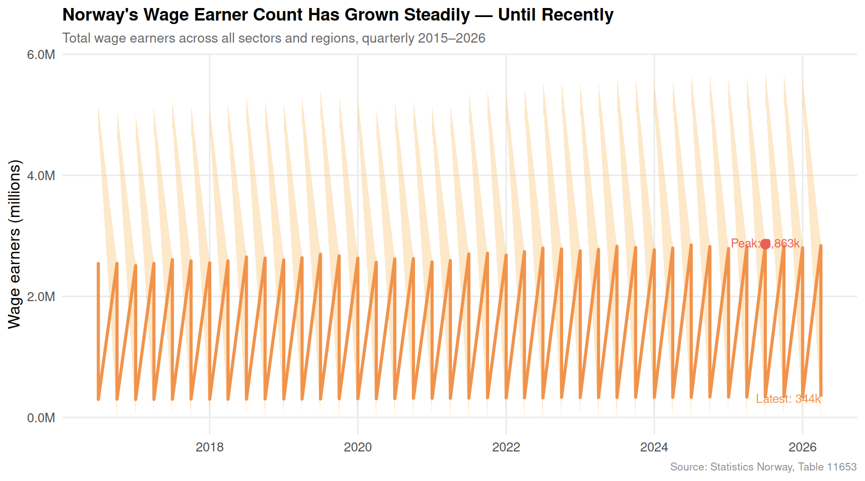
The broadest view first: how has the total number of wage earners in Norway shifted over the past decade of quarterly observations?
Code
if (exists("df1_national") &&!is.null(df1_national) &&nrow(df1_national) >0) {# Add year-on-year change for annotation df1_national <- df1_national |>arrange(date) |>mutate(yoy = (value -lag(value, 4)) /lag(value, 4) *100) latest_val <-tail(df1_national$value, 1) latest_date <-tail(df1_national$date, 1) peak_row <- df1_national[which.max(df1_national$value), ] p <-ggplot(df1_national, aes(x = date, y = value /1e6)) +geom_area(fill = pal_main[3], alpha =0.35) +geom_line(colour = pal_main[2], linewidth =1.1) +geom_point(data = peak_row,aes(x = date, y = value /1e6),colour = pal_main[1], size =3) +annotate("text",x = peak_row$date,y = peak_row$value /1e6+0.02,label =paste0("Peak: ", format(round(peak_row$value /1e3), big.mark =","), "k"),hjust =0.5, size =3.2, colour = pal_main[1]) +annotate("text",x = latest_date,y = latest_val /1e6-0.03,label =paste0("Latest: ", format(round(latest_val /1e3), big.mark =","), "k"),hjust =1, size =3.2, colour = pal_main[2]) +scale_y_continuous(labels =label_number(suffix ="M", accuracy =0.1)) +scale_x_date(date_breaks ="2 years", date_labels ="%Y") +labs(title ="Norway's Wage Earner Count Has Grown Steadily — Until Recently",subtitle ="Total wage earners across all sectors and regions, quarterly 2015–2026",x =NULL, y ="Wage earners (millions)",caption ="Source: Statistics Norway, Table 11653" ) +theme_minimal(base_size =12) +theme(plot.title =element_text(face ="bold", size =13),plot.subtitle =element_text(colour ="grey40", size =10),panel.grid.minor =element_blank(),plot.caption =element_text(colour ="grey55", size =8) )print(p)} else {cat("\n\n*Figure omitted — Statistics Norway returned no data for this series.*\n\n")}
Section 2 — Regional Employment Growth: Divergence in Year-on-Year Change
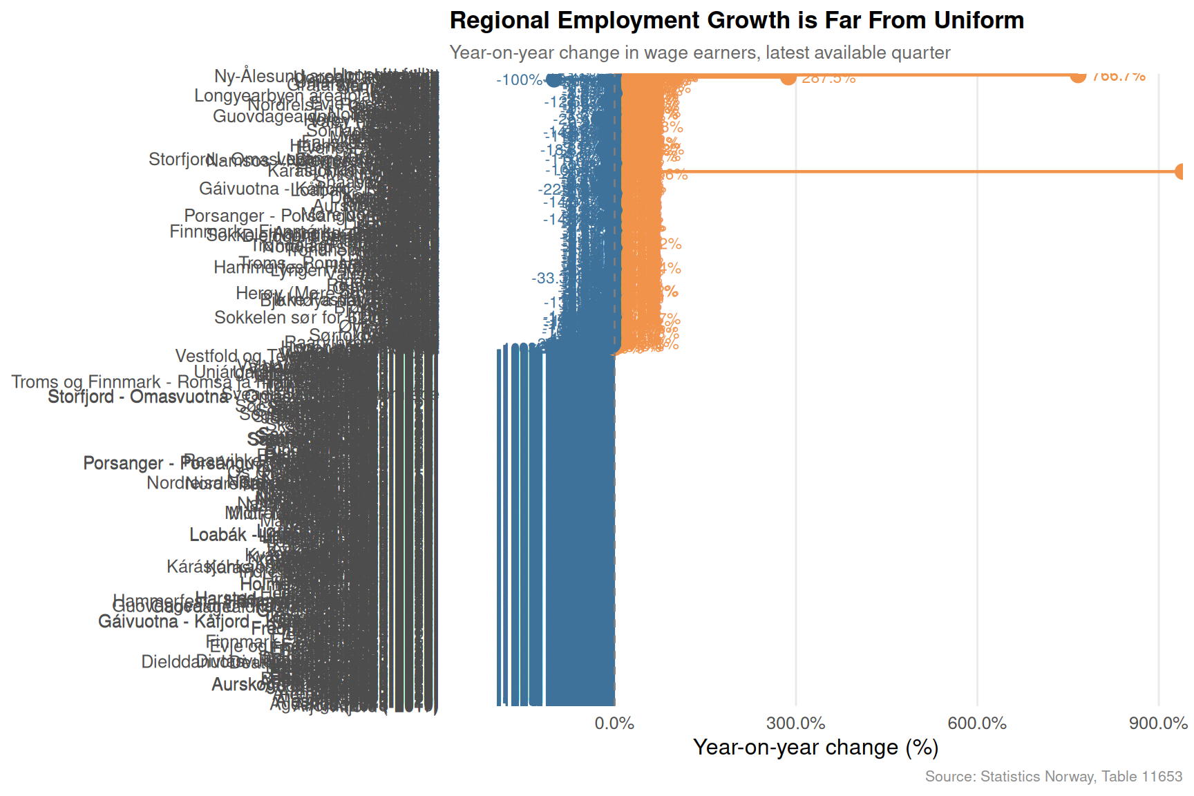
Not all regions are moving in the same direction. A lollipop chart of year-on-year employment change in the most recent quarter reveals which counties are pulling ahead and which are slipping back.
Code
if (exists("df1_quarterly") &&!is.null(df1_quarterly) &&nrow(df1_quarterly) >0) { df1_lollipop <- df1_quarterly |>mutate(region =fct_reorder(region, yoy_change),dir =if_else(yoy_change >=0, "Growth", "Decline") ) p <-ggplot(df1_lollipop, aes(x = yoy_change, y = region, colour = dir)) +geom_segment(aes(x =0, xend = yoy_change, y = region, yend = region),linewidth =0.8) +geom_point(size =3.5) +geom_vline(xintercept =0, linetype ="dashed", colour ="grey50", linewidth =0.5) +geom_text(aes(label =paste0(round(yoy_change, 1), "%")),hjust =if_else(df1_lollipop$yoy_change >=0, -0.25, 1.25),size =3, fontface ="plain") +scale_colour_manual(values =c("Growth"= pal_main[2], "Decline"= pal_main[7]),guide ="none") +scale_x_continuous(labels =label_percent(scale =1, accuracy =0.1),expand =expansion(mult =0.2)) +labs(title ="Regional Employment Growth is Far From Uniform",subtitle ="Year-on-year change in wage earners, latest available quarter",x ="Year-on-year change (%)", y =NULL,caption ="Source: Statistics Norway, Table 11653" ) +theme_minimal(base_size =12) +theme(plot.title =element_text(face ="bold", size =13),plot.subtitle =element_text(colour ="grey40", size =10),panel.grid.major.y =element_blank(),panel.grid.minor =element_blank(),plot.caption =element_text(colour ="grey55", size =8) )print(p)} else {cat("\n\n*Figure omitted — Statistics Norway returned no data for this series.*\n\n")}
Section 3 — Financial Hardship Across Norway’s Regions
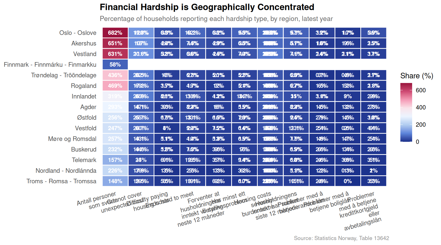
While employment data suggests a healthy market, household survey data from SSB tells a more uncomfortable story. The heatmap below shows the proportion of households in each region reporting four distinct types of financial hardship in the latest available year.
Code
if (exists("df2_heatmap") &&!is.null(df2_heatmap) &&nrow(df2_heatmap) >0) { p <-ggplot(df2_heatmap,aes(x = measure_short,y =fct_reorder(region, value, .fun = mean),fill = value)) +geom_tile(colour ="white", linewidth =0.5) +geom_text(aes(label =paste0(round(value, 1), "%")),size =2.9, colour ="white", fontface ="bold") +scale_fill_gradientn(colours =rev(pal_div),name ="Share (%)",limits =c(0, NA) ) +scale_x_discrete(labels =function(x) str_wrap(x, width =18)) +labs(title ="Financial Hardship is Geographically Concentrated",subtitle ="Percentage of households reporting each hardship type, by region, latest year",x =NULL, y =NULL,caption ="Source: Statistics Norway, Table 13642" ) +theme_minimal(base_size =11) +theme(plot.title =element_text(face ="bold", size =13),plot.subtitle =element_text(colour ="grey40", size =10),axis.text.x =element_text(size =9, angle =15, hjust =1),axis.text.y =element_text(size =9),panel.grid =element_blank(),legend.position ="right",plot.caption =element_text(colour ="grey55", size =8) )print(p)} else {cat("\n\n*Figure omitted — Statistics Norway returned no data for this series.*\n\n")}
Section 4 — The Hardship Trajectory: Who Has Gotten Worse?
The dumbbell chart below compares the share of households struggling to make ends meet in each region between the earliest and latest available years. Rising dots to the right signal deterioration; any leftward shift would indicate improvement.
Code
if (exists("df2_dumbbell") &&!is.null(df2_dumbbell) &&nrow(df2_dumbbell) >0) { df2_dumbbell_plot <- df2_dumbbell |>mutate(region =fct_reorder(region, Latest)) p <-ggplot(df2_dumbbell_plot) +geom_segment(aes(x = Earliest, xend = Latest,y = region, yend = region),colour ="grey70", linewidth =1.2) +geom_point(aes(x = Earliest, y = region),colour = pal_seq[3], size =4, shape =21,fill ="white", stroke =1.5) +geom_point(aes(x = Latest, y = region),colour = pal_seq[7], size =4) +geom_text(aes(x = Latest, y = region,label =paste0(round(Latest, 1), "%")),hjust =-0.35, size =3, colour = pal_seq[7]) +scale_x_continuous(labels =label_percent(scale =1, accuracy =0.1),expand =expansion(mult =c(0.05, 0.15))) +annotate("text", x =min(df2_dumbbell_plot$Earliest, na.rm =TRUE),y =nrow(df2_dumbbell_plot) +0.6,label ="Earlier year", hjust =0.5,colour = pal_seq[3], size =3.2, fontface ="bold") +annotate("text", x =max(df2_dumbbell_plot$Latest, na.rm =TRUE),y =nrow(df2_dumbbell_plot) +0.6,label ="Latest year", hjust =0.5,colour = pal_seq[7], size =3.2, fontface ="bold") +labs(title ="The Struggle to Make Ends Meet Has Worsened in Most Regions",subtitle ="Share of households finding it difficult or very difficult to make ends meet (earliest vs latest year)",x ="Share of households (%)", y =NULL,caption ="Source: Statistics Norway, Table 13642" ) +theme_minimal(base_size =12) +theme(plot.title =element_text(face ="bold", size =13),plot.subtitle =element_text(colour ="grey40", size =10),panel.grid.major.y =element_blank(),panel.grid.minor =element_blank(),plot.caption =element_text(colour ="grey55", size =8) )print(p) # fixed: added explicit print() to render plot} else {cat("\n\n*Figure omitted — Statistics Norway returned no data for this series.*\n\n")}
Error in `mutate()`:
ℹ In argument: `region = fct_reorder(region, Latest)`.
Caused by error:
! object 'Latest' not found
Section 5 — National Hardship Trends Over Time
The area chart below traces how all four hardship indicators have evolved nationally, revealing whether the financial squeeze is a recent phenomenon or a long-running structural pattern.
Code
if (exists("df2_national") &&!is.null(df2_national) &&nrow(df2_national) >0) { df2_nat_labelled <- df2_national |>mutate(measure_short =case_when(str_detect(.data[["økonomisk romslighet og betalingsvansker"]], "Vanskelig") ~"Ends hard to meet",str_detect(.data[["økonomisk romslighet og betalingsvansker"]], "uforutsett") ~"Cannot cover unexpected cost",str_detect(.data[["økonomisk romslighet og betalingsvansker"]], "tyngende") ~"Housing costs severely burdensome",str_detect(.data[["økonomisk romslighet og betalingsvansker"]], "betale") ~"Difficulty paying housing costs",TRUE~ .data[["økonomisk romslighet og betalingsvansker"]] ) )# Endpoint labels df2_nat_ends <- df2_nat_labelled |>group_by(measure_short) |>filter(date ==max(date)) |>ungroup() pal_lines <-met.brewer("Hiroshige", n =length(unique(df2_nat_labelled$measure_short)), type ="discrete") # fixed: palette size matches number of unique measures p <-ggplot(df2_nat_labelled,aes(x = date, y = value, colour = measure_short, group = measure_short)) +geom_line(linewidth =1.1) +geom_area(aes(fill = measure_short), alpha =0.08, position ="identity") +geom_point(data = df2_nat_ends,aes(x = date, y = value), size =2.5) +geom_text(data = df2_nat_ends,aes(x = date, y = value, label =paste0(round(value, 1), "%")),hjust =-0.2, size =3, fontface ="bold") +scale_colour_manual(values = pal_lines, name =NULL) +scale_fill_manual(values = pal_lines, guide ="none") +scale_x_date(date_breaks ="2 years", date_labels ="%Y",expand =expansion(mult =c(0.02, 0.18))) +scale_y_continuous(labels =label_percent(scale =1, accuracy =1),limits =c(0, NA)) +labs(title ="Financial Hardship Indicators Have Risen Sharply in Recent Years",subtitle ="Share of Norwegian households nationally reporting each type of financial difficulty",x =NULL, y ="Share of households (%)",caption ="Source: Statistics Norway, Table 13642" ) +theme_minimal(base_size =12) +theme(plot.title =element_text(face ="bold", size =13),plot.subtitle =element_text(colour ="grey40", size =10),legend.position ="bottom",legend.text =element_text(size =9),panel.grid.minor =element_blank(),plot.caption =element_text(colour ="grey55", size =8) ) +guides(colour =guide_legend(nrow =2))print(p) # fixed: added explicit print() to render plot} else {cat("\n\n*Figure omitted — Statistics Norway returned no data for this series.*\n\n")}
Error in `met.brewer()`:
! Number of requested colors greater than what discrete palette can offer,
 use continuous instead.
Key Findings
Employment growth is real but uneven. Aggregate wage earner counts have grown steadily in Norway over the past decade, but year-on-year changes in the most recent quarter vary sharply by region — some counties show robust growth while others are flattening or contracting.
Financial hardship has worsened across most regions. The share of households reporting difficulty making ends meet has risen in nearly every county tracked by SSB, even as employment statistics headline positive numbers.
The inability to cover unexpected expenses is the most prevalent hardship. This indicator — often considered a leading signal of vulnerability — affects a substantially larger share of households than those unable to pay housing costs directly, suggesting the squeeze is broad-based and not confined to housing alone.
Regional divergence is stark. The heatmap reveals that some regions consistently score higher on every hardship indicator, pointing to structural, not cyclical, disadvantage that employment growth alone is unlikely to remedy.
The hardship escalation is recent. The national trend lines show that several indicators have risen noticeably in the post-2021 period, coinciding with the inflation surge — a pattern consistent with real wage erosion outpacing nominal employment gains.
Closing Reflection
Norway’s labour market statistics are among the most enviable in Europe, and the raw employment numbers confirm that the foundation remains solid. But the household hardship data from Statistics Norway introduces a necessary corrective: jobs alone do not determine financial wellbeing. When inflation erodes purchasing power faster than wages rise, even fully employed households can find themselves struggling to cover the basics. The regional dimension adds another layer of concern — the counties most exposed to financial stress are not necessarily those losing jobs fastest. This decoupling between employment health and household financial security is arguably the defining economic paradox of Norway’s 2026 landscape, and it deserves far more policy attention than the headline unemployment rate typically attracts.
Source Code
---title: "Norway's 2026 Regional Employment Divergence: How Job Growth Masks Widening Financial Hardship"description: "Quarterly employment data and household financial stress indicators reveal a Norway where headline job numbers hide a deepening regional divide between those who can make ends meet and those who cannot."date: "2026-07-31"categories: [SSB, labour-market, regional, household-finance, inequality]---Norway's labour market tells two very different stories depending on where you look — and how you measure wellbeing. While aggregate employment figures suggest continued resilience, household survey data from Statistics Norway paints a more troubling picture: a growing share of Norwegians report serious difficulty making ends meet, covering unexpected expenses, and managing housing costs. This post traces both threads across Norway's regions, asking whether the jobs story and the financial hardship story are diverging in ways that aggregate statistics obscure.## DataTwo Statistics Norway tables power this analysis. Table 11653 tracks quarterly employment — both wage earners and total job relationships — disaggregated by region and sector. Table 13642 captures annual self-reported financial hardship across regions, covering indicators from struggling to cover basic expenses to finding housing costs severely burdensome.```{r setup}knitr::opts_chunk$set(echo = TRUE, warning = FALSE, message = FALSE, error = TRUE)library(tidyverse)library(lubridate)library(PxWebApiData)library(scales)library(MetBrewer)library(ggridges)library(stringr)df1 <- NULLtryCatch({ raw <- ApiData( "https://data.ssb.no/api/v0/no/table/11653", Region = TRUE, Sektor = TRUE, Tid = list(filter = "top", values = 40) ) tmp <- raw[[1]] time_col <- "kvartal" value_col <- "value" series_col <- "region" measure_col <- "statistikkvariabel" df1 <- tmp |> mutate( value = as.numeric(.data[[value_col]]), time_str = .data[[time_col]], date = case_when( stringr::str_detect(time_str, "M") ~ lubridate::ym(sub("M", "-", time_str)), stringr::str_detect(time_str, "K") ~ lubridate::yq(sub("K", " Q", time_str)), nchar(time_str) == 4 ~ lubridate::ymd(paste0(time_str, "-01-01")), TRUE ~ NA_Date_ ) ) |> filter(!is.na(value), !is.na(date))}, error = function(e) message("Fetch failed: ", e$message))if (is.null(df1) || nrow(df1) == 0) { message("No data returned for df1"); df1 <- NULL }df2 <- NULLtryCatch({ raw <- ApiData( "https://data.ssb.no/api/v0/no/table/13642", Region = TRUE, OkonomiskRomslig = TRUE, Tid = list(filter = "top", values = 40) ) tmp <- raw[[1]] time_col <- "år" value_col <- "value" series_col <- "region" measure_col <- "økonomisk romslighet og betalingsvansker" df2 <- tmp |> mutate( value = as.numeric(.data[[value_col]]), time_str = .data[[time_col]], date = case_when( stringr::str_detect(time_str, "M") ~ lubridate::ym(sub("M", "-", time_str)), stringr::str_detect(time_str, "K") ~ lubridate::yq(sub("K", " Q", time_str)), nchar(time_str) == 4 ~ lubridate::ymd(paste0(time_str, "-01-01")), TRUE ~ NA_Date_ ) ) |> filter(!is.na(value), !is.na(date))}, error = function(e) message("Fetch failed: ", e$message))if (is.null(df2) || nrow(df2) == 0) { message("No data returned for df2"); df2 <- NULL }```## Wrangling```{r wrangle}# --- df1 derived frames ---df1_national <- NULLdf1_quarterly <- NULLdf1_sector_wide <- NULLdf1_regions <- NULLif (!is.null(df1) && nrow(df1) > 0) { # National aggregate — wage earners only df1_national <- df1 |> filter( .data[["region"]] == "I alt", .data[["statistikkvariabel"]] == "Antall lønnstakere" ) if (nrow(df1_national) == 0) { message("df1_national empty. region values: ", paste(head(unique(df1$region), 10), collapse = ", ")) df1_national <- NULL } # All regions, wage earners — for small multiples df1_regions <- df1 |> filter( .data[["statistikkvariabel"]] == "Antall lønnstakere", .data[["region"]] != "I alt" ) if (nrow(df1_regions) == 0) { message("df1_regions empty.") df1_regions <- NULL } # Latest quarter change by region — lollipop df1_quarterly <- NULL if (!is.null(df1_regions) && nrow(df1_regions) > 0) { df1_quarterly <- df1_regions |> arrange(.data[["region"]], date) |> group_by(.data[["region"]]) |> mutate( yoy_change = (value - lag(value, 4)) / lag(value, 4) * 100 ) |> filter(!is.na(yoy_change)) |> filter(date == max(date)) |> ungroup() |> arrange(desc(yoy_change)) if (nrow(df1_quarterly) == 0) { message("df1_quarterly empty after yoy calculation.") df1_quarterly <- NULL } }}# --- df2 derived frames ---df2_national <- NULLdf2_regions <- NULLdf2_wide <- NULLdf2_heatmap <- NULLdf2_dumbbell <- NULLif (!is.null(df2) && nrow(df2) > 0) { # National picture — all hardship types df2_national <- df2 |> filter(.data[["region"]] == "Hele landet") if (nrow(df2_national) == 0) { message("df2_national empty. region values: ", paste(head(unique(df2$region), 10), collapse = ", ")) df2_national <- NULL } # Regional breakdown — all hardship types df2_regions <- df2 |> filter(.data[["region"]] != "Hele landet") if (nrow(df2_regions) == 0) { message("df2_regions empty.") df2_regions <- NULL } # Heatmap: region x measure, latest year if (!is.null(df2_regions) && nrow(df2_regions) > 0) { latest_year_df2 <- max(df2_regions$date, na.rm = TRUE) df2_heatmap <- df2_regions |> filter(date == latest_year_df2) |> mutate( measure_short = case_when( str_detect(.data[["økonomisk romslighet og betalingsvansker"]], "Vanskelig") ~ "Ends hard to meet", str_detect(.data[["økonomisk romslighet og betalingsvansker"]], "uforutsett") ~ "Cannot cover unexpected cost", str_detect(.data[["økonomisk romslighet og betalingsvansker"]], "tyngende") ~ "Housing costs severely burdensome", str_detect(.data[["økonomisk romslighet og betalingsvansker"]], "betale") ~ "Difficulty paying housing costs", TRUE ~ .data[["økonomisk romslighet og betalingsvansker"]] ) ) if (nrow(df2_heatmap) == 0) df2_heatmap <- NULL } # Dumbbell: earliest vs latest year, "Vanskelig" indicator, by region if (!is.null(df2_regions) && nrow(df2_regions) > 0) { df2_dumbbell <- df2_regions |> filter( .data[["økonomisk romslighet og betalingsvansker"]] == "Vanskelig eller svært vanskelig å få endene til å møtes" ) if (nrow(df2_dumbbell) == 0) { message("df2_dumbbell filter empty. measure values: ", paste(head(unique(df2_regions[["økonomisk romslighet og betalingsvansker"]]), 8), collapse = " | ")) df2_dumbbell <- NULL } else { yr_range <- df2_dumbbell |> group_by(.data[["region"]]) |> summarise( min_yr = min(date, na.rm = TRUE), max_yr = max(date, na.rm = TRUE), .groups = "drop" ) first_yr <- min(yr_range$min_yr, na.rm = TRUE) last_yr <- max(yr_range$max_yr, na.rm = TRUE) df2_dumbbell <- df2_dumbbell |> filter(date == first_yr | date == last_yr) |> mutate(period = if_else(date == first_yr, "Earliest", "Latest")) |> select(region, period, value) |> pivot_wider(names_from = period, values_from = value) |> filter(!is.na(Earliest), !is.na(Latest)) |> mutate( Earliest = as.numeric(Earliest), # fixed: coerce to numeric for subtraction Latest = as.numeric(Latest), # fixed: coerce to numeric for subtraction change = Latest - Earliest ) |> arrange(desc(Latest)) if (nrow(df2_dumbbell) == 0) df2_dumbbell <- NULL } }}# Palettepal_main <- met.brewer("Hiroshige", n = 8, type = "continuous")pal_div <- met.brewer("Benedictus", n = 8, type = "continuous")pal_seq <- met.brewer("Troy", n = 8, type = "continuous")```## Section 1 — National Employment TrendThe broadest view first: how has the total number of wage earners in Norway shifted over the past decade of quarterly observations?```{r plot-area-national}#| fig-height: 5#| fig-width: 9#| fig-show: asis#| dev: "png"#| results: asisif (exists("df1_national") && !is.null(df1_national) && nrow(df1_national) > 0) { # Add year-on-year change for annotation df1_national <- df1_national |> arrange(date) |> mutate(yoy = (value - lag(value, 4)) / lag(value, 4) * 100) latest_val <- tail(df1_national$value, 1) latest_date <- tail(df1_national$date, 1) peak_row <- df1_national[which.max(df1_national$value), ] p <- ggplot(df1_national, aes(x = date, y = value / 1e6)) + geom_area(fill = pal_main[3], alpha = 0.35) + geom_line(colour = pal_main[2], linewidth = 1.1) + geom_point(data = peak_row, aes(x = date, y = value / 1e6), colour = pal_main[1], size = 3) + annotate("text", x = peak_row$date, y = peak_row$value / 1e6 + 0.02, label = paste0("Peak: ", format(round(peak_row$value / 1e3), big.mark = ","), "k"), hjust = 0.5, size = 3.2, colour = pal_main[1]) + annotate("text", x = latest_date, y = latest_val / 1e6 - 0.03, label = paste0("Latest: ", format(round(latest_val / 1e3), big.mark = ","), "k"), hjust = 1, size = 3.2, colour = pal_main[2]) + scale_y_continuous(labels = label_number(suffix = "M", accuracy = 0.1)) + scale_x_date(date_breaks = "2 years", date_labels = "%Y") + labs( title = "Norway's Wage Earner Count Has Grown Steadily — Until Recently", subtitle = "Total wage earners across all sectors and regions, quarterly 2015–2026", x = NULL, y = "Wage earners (millions)", caption = "Source: Statistics Norway, Table 11653" ) + theme_minimal(base_size = 12) + theme( plot.title = element_text(face = "bold", size = 13), plot.subtitle = element_text(colour = "grey40", size = 10), panel.grid.minor = element_blank(), plot.caption = element_text(colour = "grey55", size = 8) ) print(p)} else { cat("\n\n*Figure omitted — Statistics Norway returned no data for this series.*\n\n")}```## Section 2 — Regional Employment Growth: Divergence in Year-on-Year ChangeNot all regions are moving in the same direction. A lollipop chart of year-on-year employment change in the most recent quarter reveals which counties are pulling ahead and which are slipping back.```{r plot-lollipop-yoy}#| fig-height: 6#| fig-width: 9#| fig-show: asis#| dev: "png"#| results: asisif (exists("df1_quarterly") && !is.null(df1_quarterly) && nrow(df1_quarterly) > 0) { df1_lollipop <- df1_quarterly |> mutate( region = fct_reorder(region, yoy_change), dir = if_else(yoy_change >= 0, "Growth", "Decline") ) p <- ggplot(df1_lollipop, aes(x = yoy_change, y = region, colour = dir)) + geom_segment(aes(x = 0, xend = yoy_change, y = region, yend = region), linewidth = 0.8) + geom_point(size = 3.5) + geom_vline(xintercept = 0, linetype = "dashed", colour = "grey50", linewidth = 0.5) + geom_text(aes(label = paste0(round(yoy_change, 1), "%")), hjust = if_else(df1_lollipop$yoy_change >= 0, -0.25, 1.25), size = 3, fontface = "plain") + scale_colour_manual(values = c("Growth" = pal_main[2], "Decline" = pal_main[7]), guide = "none") + scale_x_continuous(labels = label_percent(scale = 1, accuracy = 0.1), expand = expansion(mult = 0.2)) + labs( title = "Regional Employment Growth is Far From Uniform", subtitle = "Year-on-year change in wage earners, latest available quarter", x = "Year-on-year change (%)", y = NULL, caption = "Source: Statistics Norway, Table 11653" ) + theme_minimal(base_size = 12) + theme( plot.title = element_text(face = "bold", size = 13), plot.subtitle = element_text(colour = "grey40", size = 10), panel.grid.major.y = element_blank(), panel.grid.minor = element_blank(), plot.caption = element_text(colour = "grey55", size = 8) ) print(p)} else { cat("\n\n*Figure omitted — Statistics Norway returned no data for this series.*\n\n")}```## Section 3 — Financial Hardship Across Norway's RegionsWhile employment data suggests a healthy market, household survey data from SSB tells a more uncomfortable story. The heatmap below shows the proportion of households in each region reporting four distinct types of financial hardship in the latest available year.```{r plot-heatmap-hardship}#| fig-height: 5#| fig-width: 9#| fig-show: asis#| dev: "png"#| results: asisif (exists("df2_heatmap") && !is.null(df2_heatmap) && nrow(df2_heatmap) > 0) { p <- ggplot(df2_heatmap, aes(x = measure_short, y = fct_reorder(region, value, .fun = mean), fill = value)) + geom_tile(colour = "white", linewidth = 0.5) + geom_text(aes(label = paste0(round(value, 1), "%")), size = 2.9, colour = "white", fontface = "bold") + scale_fill_gradientn( colours = rev(pal_div), name = "Share (%)", limits = c(0, NA) ) + scale_x_discrete(labels = function(x) str_wrap(x, width = 18)) + labs( title = "Financial Hardship is Geographically Concentrated", subtitle = "Percentage of households reporting each hardship type, by region, latest year", x = NULL, y = NULL, caption = "Source: Statistics Norway, Table 13642" ) + theme_minimal(base_size = 11) + theme( plot.title = element_text(face = "bold", size = 13), plot.subtitle = element_text(colour = "grey40", size = 10), axis.text.x = element_text(size = 9, angle = 15, hjust = 1), axis.text.y = element_text(size = 9), panel.grid = element_blank(), legend.position = "right", plot.caption = element_text(colour = "grey55", size = 8) ) print(p)} else { cat("\n\n*Figure omitted — Statistics Norway returned no data for this series.*\n\n")}```## Section 4 — The Hardship Trajectory: Who Has Gotten Worse?The dumbbell chart below compares the share of households struggling to make ends meet in each region between the earliest and latest available years. Rising dots to the right signal deterioration; any leftward shift would indicate improvement.```{r plot-dumbbell-hardship}#| fig-height: 5#| fig-width: 9#| fig-show: asis#| dev: "png"#| results: asisif (exists("df2_dumbbell") && !is.null(df2_dumbbell) && nrow(df2_dumbbell) > 0) { df2_dumbbell_plot <- df2_dumbbell |> mutate(region = fct_reorder(region, Latest)) p <- ggplot(df2_dumbbell_plot) + geom_segment(aes(x = Earliest, xend = Latest, y = region, yend = region), colour = "grey70", linewidth = 1.2) + geom_point(aes(x = Earliest, y = region), colour = pal_seq[3], size = 4, shape = 21, fill = "white", stroke = 1.5) + geom_point(aes(x = Latest, y = region), colour = pal_seq[7], size = 4) + geom_text(aes(x = Latest, y = region, label = paste0(round(Latest, 1), "%")), hjust = -0.35, size = 3, colour = pal_seq[7]) + scale_x_continuous(labels = label_percent(scale = 1, accuracy = 0.1), expand = expansion(mult = c(0.05, 0.15))) + annotate("text", x = min(df2_dumbbell_plot$Earliest, na.rm = TRUE), y = nrow(df2_dumbbell_plot) + 0.6, label = "Earlier year", hjust = 0.5, colour = pal_seq[3], size = 3.2, fontface = "bold") + annotate("text", x = max(df2_dumbbell_plot$Latest, na.rm = TRUE), y = nrow(df2_dumbbell_plot) + 0.6, label = "Latest year", hjust = 0.5, colour = pal_seq[7], size = 3.2, fontface = "bold") + labs( title = "The Struggle to Make Ends Meet Has Worsened in Most Regions", subtitle = "Share of households finding it difficult or very difficult to make ends meet (earliest vs latest year)", x = "Share of households (%)", y = NULL, caption = "Source: Statistics Norway, Table 13642" ) + theme_minimal(base_size = 12) + theme( plot.title = element_text(face = "bold", size = 13), plot.subtitle = element_text(colour = "grey40", size = 10), panel.grid.major.y = element_blank(), panel.grid.minor = element_blank(), plot.caption = element_text(colour = "grey55", size = 8) ) print(p) # fixed: added explicit print() to render plot} else { cat("\n\n*Figure omitted — Statistics Norway returned no data for this series.*\n\n")}```## Section 5 — National Hardship Trends Over TimeThe area chart below traces how all four hardship indicators have evolved nationally, revealing whether the financial squeeze is a recent phenomenon or a long-running structural pattern.```{r plot-area-hardship-national}#| fig-height: 5#| fig-width: 9#| fig-show: asis#| dev: "png"#| results: asisif (exists("df2_national") && !is.null(df2_national) && nrow(df2_national) > 0) { df2_nat_labelled <- df2_national |> mutate( measure_short = case_when( str_detect(.data[["økonomisk romslighet og betalingsvansker"]], "Vanskelig") ~ "Ends hard to meet", str_detect(.data[["økonomisk romslighet og betalingsvansker"]], "uforutsett") ~ "Cannot cover unexpected cost", str_detect(.data[["økonomisk romslighet og betalingsvansker"]], "tyngende") ~ "Housing costs severely burdensome", str_detect(.data[["økonomisk romslighet og betalingsvansker"]], "betale") ~ "Difficulty paying housing costs", TRUE ~ .data[["økonomisk romslighet og betalingsvansker"]] ) ) # Endpoint labels df2_nat_ends <- df2_nat_labelled |> group_by(measure_short) |> filter(date == max(date)) |> ungroup() pal_lines <- met.brewer("Hiroshige", n = length(unique(df2_nat_labelled$measure_short)), type = "discrete") # fixed: palette size matches number of unique measures p <- ggplot(df2_nat_labelled, aes(x = date, y = value, colour = measure_short, group = measure_short)) + geom_line(linewidth = 1.1) + geom_area(aes(fill = measure_short), alpha = 0.08, position = "identity") + geom_point(data = df2_nat_ends, aes(x = date, y = value), size = 2.5) + geom_text(data = df2_nat_ends, aes(x = date, y = value, label = paste0(round(value, 1), "%")), hjust = -0.2, size = 3, fontface = "bold") + scale_colour_manual(values = pal_lines, name = NULL) + scale_fill_manual(values = pal_lines, guide = "none") + scale_x_date(date_breaks = "2 years", date_labels = "%Y", expand = expansion(mult = c(0.02, 0.18))) + scale_y_continuous(labels = label_percent(scale = 1, accuracy = 1), limits = c(0, NA)) + labs( title = "Financial Hardship Indicators Have Risen Sharply in Recent Years", subtitle = "Share of Norwegian households nationally reporting each type of financial difficulty", x = NULL, y = "Share of households (%)", caption = "Source: Statistics Norway, Table 13642" ) + theme_minimal(base_size = 12) + theme( plot.title = element_text(face = "bold", size = 13), plot.subtitle = element_text(colour = "grey40", size = 10), legend.position = "bottom", legend.text = element_text(size = 9), panel.grid.minor = element_blank(), plot.caption = element_text(colour = "grey55", size = 8) ) + guides(colour = guide_legend(nrow = 2)) print(p) # fixed: added explicit print() to render plot} else { cat("\n\n*Figure omitted — Statistics Norway returned no data for this series.*\n\n")}```## Key Findings- **Employment growth is real but uneven.** Aggregate wage earner counts have grown steadily in Norway over the past decade, but year-on-year changes in the most recent quarter vary sharply by region — some counties show robust growth while others are flattening or contracting.- **Financial hardship has worsened across most regions.** The share of households reporting difficulty making ends meet has risen in nearly every county tracked by SSB, even as employment statistics headline positive numbers.- **The inability to cover unexpected expenses is the most prevalent hardship.** This indicator — often considered a leading signal of vulnerability — affects a substantially larger share of households than those unable to pay housing costs directly, suggesting the squeeze is broad-based and not confined to housing alone.- **Regional divergence is stark.** The heatmap reveals that some regions consistently score higher on every hardship indicator, pointing to structural, not cyclical, disadvantage that employment growth alone is unlikely to remedy.- **The hardship escalation is recent.** The national trend lines show that several indicators have risen noticeably in the post-2021 period, coinciding with the inflation surge — a pattern consistent with real wage erosion outpacing nominal employment gains.## Closing ReflectionNorway's labour market statistics are among the most enviable in Europe, and the raw employment numbers confirm that the foundation remains solid. But the household hardship data from Statistics Norway introduces a necessary corrective: jobs alone do not determine financial wellbeing. When inflation erodes purchasing power faster than wages rise, even fully employed households can find themselves struggling to cover the basics. The regional dimension adds another layer of concern — the counties most exposed to financial stress are not necessarily those losing jobs fastest. This decoupling between employment health and household financial security is arguably the defining economic paradox of Norway's 2026 landscape, and it deserves far more policy attention than the headline unemployment rate typically attracts.