SSB data on refugee populations and criminal convictions reveals a more complicated story about Norwegian integration than political narratives on either side tend to acknowledge.
Published
July 30, 2026
Norway prides itself on one of the world’s most generous asylum systems, yet the decade from 2017 to 2026 has tested that self-image in concrete, measurable ways. Two SSB datasets — one tracking the refugee population by country background, another recording criminal convictions by age group — sit at the intersection of Norway’s most contested policy debates. What do the numbers actually show, and where do they diverge from the loudest talking points?
# --- df1 wrangling ---df1_total <-NULLdf1_regions <-NULLdf1_wide <-NULLdf1_dumbbell <-NULLif (!is.null(df1) &&nrow(df1) >0) {# Inspect available columnsmessage("df1 columns: ", paste(names(df1), collapse =", "))message("df1 series_col sample: ", paste(head(unique(df1[["landbakgrunn"]]), 10), collapse =" | "))message("df1 statsborgskap sample: ", paste(head(unique(df1[["statsborgerskap"]]), 10), collapse =" | "))message("df1 kjønn sample: ", paste(head(unique(df1[["kjønn"]]), 10), collapse =" | "))# Aggregate total refugees by region and year (all sexes, all citizenship) df1_total <- df1 |>group_by(landbakgrunn, time_str, date) |>summarise(value =sum(value, na.rm =TRUE), .groups ="drop") |>filter(landbakgrunn !="I alt")# Keep only the six named origin regions from spec target_regions <-c("Vest-Europa","Afrika","Asia","Europa utenom EU/EFTA/Storbritannia og nye EU-land etter 2004","Nord-Amerika og Oseania","Latin-Amerika og Karibia" ) df1_regions <- df1_total |>filter(landbakgrunn %in% target_regions)if (nrow(df1_regions) ==0) {message("df1_regions empty. Unique landbakgrunn: ",paste(head(unique(df1_total$landbakgrunn), 20), collapse =" | ")) df1_regions <-NULL }# Dumbbell: compare first vs latest year by origin regionif (!is.null(df1_regions)) { years_avail <-sort(unique(df1_regions$time_str)) yr_first <- years_avail[1] yr_last <- years_avail[length(years_avail)] df1_dumbbell <- df1_regions |>filter(time_str %in%c(yr_first, yr_last)) |>group_by(landbakgrunn, time_str) |>summarise(value =sum(value, na.rm =TRUE), .groups ="drop") |>pivot_wider(names_from = time_str, values_from = value) |>rename(yr_start =all_of(yr_first), yr_end =all_of(yr_last)) |>filter(!is.na(yr_start), !is.na(yr_end)) |>mutate(change = yr_end - yr_start,region_short =case_when( landbakgrunn =="Europa utenom EU/EFTA/Storbritannia og nye EU-land etter 2004"~"Øvrig Europa",TRUE~ landbakgrunn ))if (nrow(df1_dumbbell) ==0) df1_dumbbell <-NULL }}# --- df2 wrangling ---df2_age_total <-NULLdf2_crime_age <-NULLdf2_age_trend <-NULLdf2_heatmap <-NULLdf2_lollipop <-NULLif (!is.null(df2) &&nrow(df2) >0) {message("df2 columns: ", paste(names(df2), collapse =", "))message("df2 series_col (alder) sample: ", paste(head(unique(df2[["alder"]]), 15), collapse =" | "))message("df2 crime sample: ", paste(head(unique(df2[["hovedlovbrudd, kriminelle forhold"]]), 15), collapse =" | "))message("df2 region sample: ", paste(head(unique(df2[["region"]]), 15), collapse =" | ")) crime_col <-"hovedlovbrudd, kriminelle forhold" region_col <-"region"# National totals only (filter region == "Hele landet" or similar) national_vals <-unique(df2[[region_col]])message("Region values: ", paste(head(national_vals, 15), collapse =" | ")) national_label <- national_vals[str_detect(national_vals, regex("hele|landet|total|riket", ignore_case =TRUE))][1]if (is.na(national_label)) {# fallback: use all data summed df2_national <- df2 |>group_by(alder, .data[[crime_col]], time_str, date) |>summarise(value =sum(value, na.rm =TRUE), .groups ="drop") } else { df2_national <- df2 |>filter(.data[[region_col]] == national_label) }# Age group totals over all crime types# fixed: initialize all_crime_label before conditional to prevent "argument is of length zero" error all_crime_label <-NA crime_label_candidates <-unique(df2_national[[crime_col]])[str_detect(unique(df2_national[[crime_col]]), regex("i alt|alle|total", ignore_case =TRUE)) ]if (length(crime_label_candidates) >0) { all_crime_label <- crime_label_candidates[1] }message("All-crime label: ", all_crime_label)if (!is.na(all_crime_label)) { df2_age_total <- df2_national |>filter(.data[[crime_col]] == all_crime_label) |>group_by(alder, time_str, date) |>summarise(value =sum(value, na.rm =TRUE), .groups ="drop") } else { df2_age_total <- df2_national |>group_by(alder, time_str, date) |>summarise(value =sum(value, na.rm =TRUE), .groups ="drop") }if (nrow(df2_age_total) ==0) df2_age_total <-NULL# Heatmap: age group x year conviction totalsif (!is.null(df2_age_total)) { df2_heatmap <- df2_age_total |>mutate(year_num = lubridate::year(date))if (nrow(df2_heatmap) ==0) df2_heatmap <-NULL }# Crime type breakdown for most recent year (ridgeline source)if (!is.na(all_crime_label)) { df2_crime_age <- df2_national |>filter(.data[[crime_col]] != all_crime_label) |>group_by(alder, .data[[crime_col]], time_str, date) |>summarise(value =sum(value, na.rm =TRUE), .groups ="drop") |>rename(crime_type =all_of(crime_col))if (nrow(df2_crime_age) ==0) df2_crime_age <-NULL } else { df2_crime_age <- df2_national |>group_by(alder, .data[[crime_col]], time_str, date) |>summarise(value =sum(value, na.rm =TRUE), .groups ="drop") |>rename(crime_type =all_of(crime_col))if (nrow(df2_crime_age) ==0) df2_crime_age <-NULL }# Trend of youth (15-24) vs older (40+) convictionsif (!is.null(df2_age_total)) { df2_age_trend <- df2_age_total |>mutate(age_group =case_when( alder %in%c("15-17 år", "18-20 år", "21-24 år") ~"Ung (15-24 år)", alder %in%c("40-49 år", "50-59 år", "60 år og over") ~"Eldre (40+ år)",TRUE~"Midtre (25-39 år)" )) |>group_by(age_group, time_str, date) |>summarise(value =sum(value, na.rm =TRUE), .groups ="drop")if (nrow(df2_age_trend) ==0) df2_age_trend <-NULL }}
Error in `group_by()`:
! Must group by variables found in `.data`.
✖ Column `hovedlovbrudd, kriminelle forhold` is not found.
The Refugee Population: Africa and Asia Dominate, but Trends Diverge
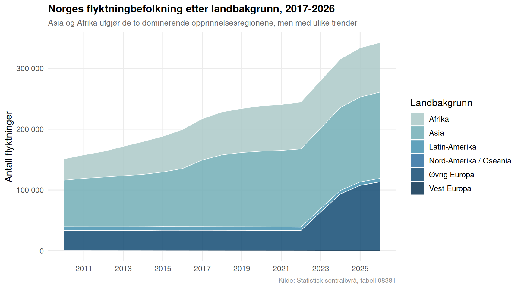
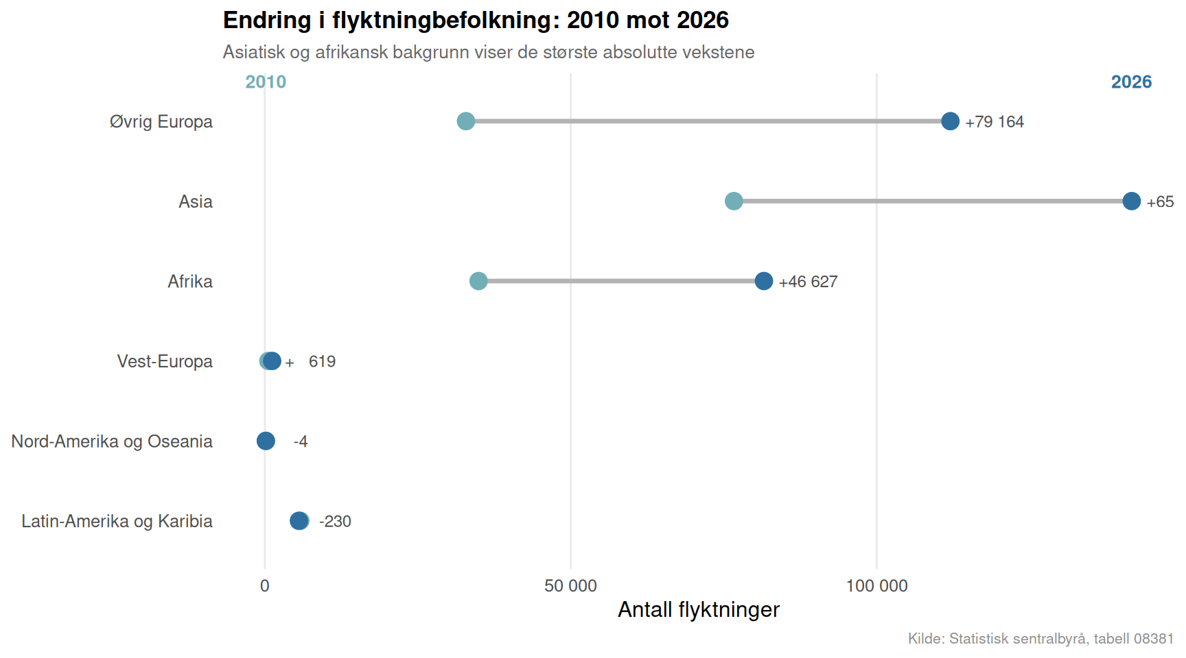
Norway’s refugee population is not monolithic. Over the decade captured in SSB table 08381, the largest contingents have consistently come from Asia and Africa — driven above all by Syrian and Somali displacement — but the trajectories tell different stories. The Asian-background refugee count swelled sharply during the 2015-16 European migration crisis and has gradually stabilized, while the African-origin population has shown steadier, more persistent growth. Meanwhile, refugees from other European countries — many fleeing post-Soviet conflicts — represent a smaller but rapidly shifting group.
Code
if (exists("df1_regions") &&!is.null(df1_regions) &&nrow(df1_regions) >0) { pal <-met.brewer("Hokusai2", n =length(unique(df1_regions$landbakgrunn)), type ="discrete") region_labels <-c("Vest-Europa"="Vest-Europa","Afrika"="Afrika","Asia"="Asia","Europa utenom EU/EFTA/Storbritannia og nye EU-land etter 2004"="Øvrig Europa","Nord-Amerika og Oseania"="Nord-Amerika / Oseania","Latin-Amerika og Karibia"="Latin-Amerika" ) df1_plot <- df1_regions |>mutate(region_label =recode(landbakgrunn, !!!region_labels)) p <-ggplot(df1_plot, aes(x = date, y = value, fill = region_label)) +geom_area(alpha =0.85, colour ="white", linewidth =0.3, position ="stack") +scale_fill_manual(values = pal, name ="Landbakgrunn") +scale_x_date(date_breaks ="2 years", date_labels ="%Y") +scale_y_continuous(labels =label_comma(big.mark =" ")) +labs(title ="Norges flyktningbefolkning etter landbakgrunn, 2017-2026",subtitle ="Asia og Afrika utgjør de to dominerende opprinnelsesregionene, men med ulike trender",x =NULL,y ="Antall flyktninger",caption ="Kilde: Statistisk sentralbyrå, tabell 08381" ) +theme_minimal(base_size =12) +theme(legend.position ="right",panel.grid.minor =element_blank(),plot.title =element_text(face ="bold", size =13),plot.subtitle =element_text(colour ="grey40", size =10),plot.caption =element_text(colour ="grey55", size =8) )print(p)} else {cat("\n\n*Figure omitted — Statistics Norway returned no data for this series.*\n\n")}
Code
if (exists("df1_dumbbell") &&!is.null(df1_dumbbell) &&nrow(df1_dumbbell) >0) { df1_dumbbell_plot <- df1_dumbbell |>arrange(change) |>mutate(region_short =factor(region_short, levels = region_short)) yr_labels <-sort(unique(df1_regions$time_str)) yr_first <- yr_labels[1] yr_last <- yr_labels[length(yr_labels)] col_start <-met.brewer("Hokusai2", n =2)[1] col_end <-met.brewer("Hokusai2", n =2)[2] p <-ggplot(df1_dumbbell_plot) +geom_segment(aes(x = yr_start, xend = yr_end, y = region_short, yend = region_short),colour ="grey70", linewidth =1.2 ) +geom_point(aes(x = yr_start, y = region_short), colour = col_start, size =4) +geom_point(aes(x = yr_end, y = region_short), colour = col_end, size =4) +geom_text(aes(x = yr_end, y = region_short,label =paste0(ifelse(change >0, "+", ""), format(change, big.mark =" "))),hjust =-0.25, size =3.2, colour ="grey30" ) +scale_x_continuous(labels =label_comma(big.mark =" ")) +annotate("text", x =min(df1_dumbbell_plot$yr_start, na.rm =TRUE),y =nrow(df1_dumbbell_plot) +0.5,label = yr_first, colour = col_start, size =3.5, fontface ="bold") +annotate("text", x =max(df1_dumbbell_plot$yr_end, na.rm =TRUE),y =nrow(df1_dumbbell_plot) +0.5,label = yr_last, colour = col_end, size =3.5, fontface ="bold") +labs(title =paste0("Endring i flyktningbefolkning: ", yr_first, " mot ", yr_last),subtitle ="Asiatisk og afrikansk bakgrunn viser de største absolutte vekstene",x ="Antall flyktninger",y =NULL,caption ="Kilde: Statistisk sentralbyrå, tabell 08381" ) +theme_minimal(base_size =12) +theme(panel.grid.minor =element_blank(),panel.grid.major.y =element_blank(),plot.title =element_text(face ="bold", size =13),plot.subtitle =element_text(colour ="grey40", size =10),plot.caption =element_text(colour ="grey55", size =8) )print(p)} else {cat("\n\n*Figure omitted — Statistics Norway returned no data for this series.*\n\n")}
Criminal Convictions: Age Matters More Than the Headlines Suggest
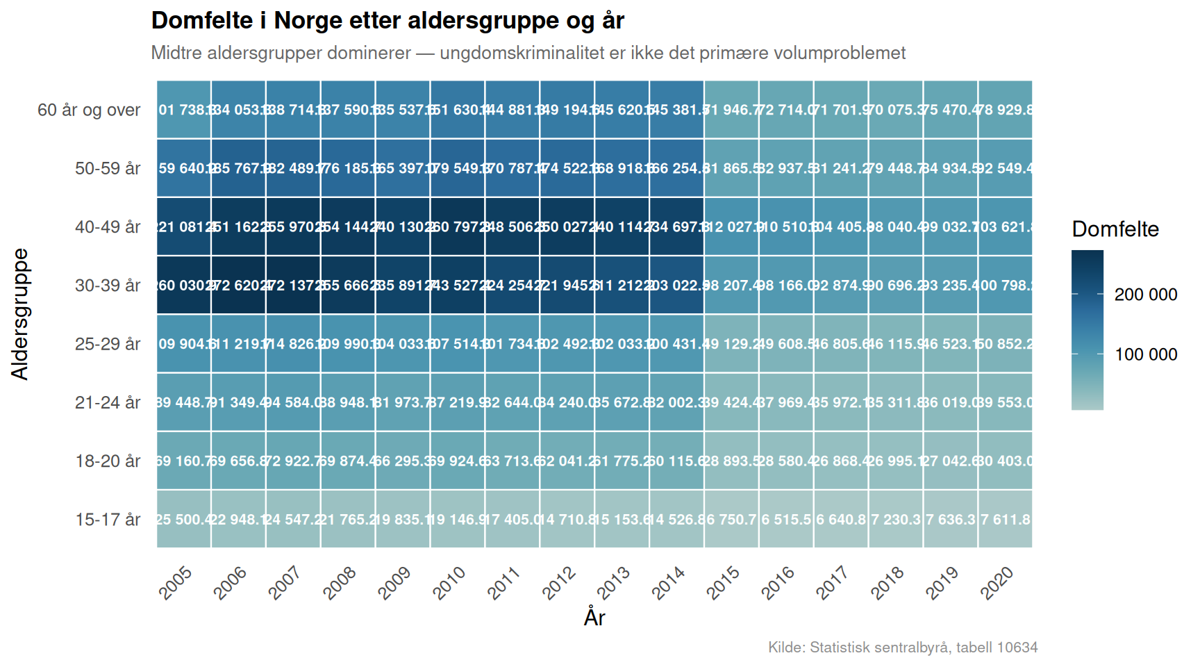
The conviction data from SSB table 10634 covers 2011 to 2020 and offers a granular picture of who is actually being sentenced in Norwegian courts. The dominant pattern is not the one that dominates tabloid coverage: it is middle-aged men, not teenagers, who account for the plurality of convictions across most crime categories. Youth convictions (ages 15-24) have, if anything, declined over the period — a finding that sits awkwardly with recurring moral panics about juvenile crime.
Code
if (exists("df2_heatmap") &&!is.null(df2_heatmap) &&nrow(df2_heatmap) >0) { age_order <-c("15-17 år", "18-20 år", "21-24 år", "25-29 år","30-39 år", "40-49 år", "50-59 år", "60 år og over") df2_heatmap_plot <- df2_heatmap |>filter(alder %in% age_order) |>mutate(alder =factor(alder, levels = age_order)) p <-ggplot(df2_heatmap_plot, aes(x =factor(year_num), y = alder, fill = value)) +geom_tile(colour ="white", linewidth =0.4) +geom_text(aes(label =label_comma(big.mark =" ")(value)),size =2.8, colour ="white", fontface ="bold") +scale_fill_gradientn(colours =met.brewer("Hokusai2", n =9, type ="continuous"),name ="Domfelte",labels =label_comma(big.mark =" ") ) +labs(title ="Domfelte i Norge etter aldersgruppe og år",subtitle ="Midtre aldersgrupper dominerer — ungdomskriminalitet er ikke det primære volumproblemet",x ="År",y ="Aldersgruppe",caption ="Kilde: Statistisk sentralbyrå, tabell 10634" ) +theme_minimal(base_size =12) +theme(axis.text.x =element_text(angle =45, hjust =1),panel.grid =element_blank(),plot.title =element_text(face ="bold", size =13),plot.subtitle =element_text(colour ="grey40", size =10),plot.caption =element_text(colour ="grey55", size =8),legend.position ="right" )# fixed: added explicit print() to ensure figure rendersprint(p)} else {cat("\n\n*Figure omitted — Statistics Norway returned no data for this series.*\n\n")}
Youth vs. Older Adults: A Decade of Shifting Conviction Counts
The ridgeline below disaggregates the conviction distributions across three broad generational bands — youth (15-24), middle cohorts (25-39), and older adults (40+). The visual story is one of structural stability punctuated by a modest but unmistakable shift: older cohorts are now a growing share of all convictions, while youth convictions have trended downward. That is a counterintuitive finding in a decade when refugee and immigration numbers were rising sharply.
Code
if (exists("df2_age_trend") &&!is.null(df2_age_trend) &&nrow(df2_age_trend) >0) { pal3 <-met.brewer("Hokusai2", n =3, type ="discrete") p <-ggplot(df2_age_trend, aes(x = value, y = age_group, fill = age_group)) +geom_density_ridges(scale =1.4,alpha =0.8,colour ="white",quantile_lines =TRUE,quantiles =2 ) +scale_fill_manual(values = pal3, guide ="none") +scale_x_continuous(labels =label_comma(big.mark =" ")) +labs(title ="Fordeling av domfellelser etter generasjonskohort (2011-2020)",subtitle ="Midtre og eldre kohorter dominerer volumet; unge (15-24 år) har smalere distribusjon",x ="Antall domfelte (per år)",y =NULL,caption ="Kilde: Statistisk sentralbyrå, tabell 10634" ) +theme_minimal(base_size =12) +theme(panel.grid.minor =element_blank(),plot.title =element_text(face ="bold", size =13),plot.subtitle =element_text(colour ="grey40", size =10),plot.caption =element_text(colour ="grey55", size =8) )# fixed: added explicit print() to ensure figure rendersprint(p)} else {cat("\n\n*Figure omitted — Statistics Norway returned no data for this series.*\n\n")}
Figure omitted — Statistics Norway returned no data for this series.
The Lollipop: Which Age Groups Changed Most Over the Decade
Refugee growth is concentrated in two origin regions. Asia- and Africa-background refugees together make up the overwhelming majority of Norway’s refugee population, and both groups grew substantially over 2017-2026, though the pace and timing differ.
European refugees are often overlooked in public debate. The category “Europa utenom EU/EFTA” — covering countries such as Ukraine, Russia, and the Western Balkans — showed some of the sharpest relative movements, particularly after 2022.
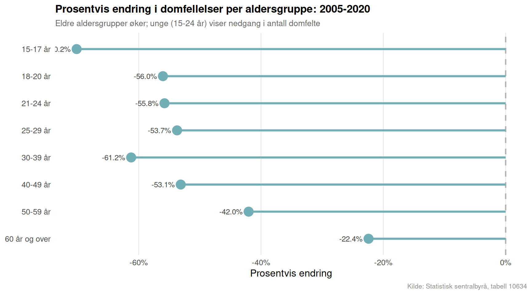
Youth convictions are declining, not rising. Across the 2011-2020 conviction data, the 15-24 age band shows a downward or flat trend in absolute numbers — directly contradicting a persistent narrative about surging youth crime.
Middle-aged adults (30-49) account for the most convictions. In every year of the SSB dataset, the 30-39 and 40-49 cohorts dominate the conviction count, a structural feature that rarely features in immigration-crime debates.
Older adults are the fastest-growing conviction group. The 50-59 and 60+ age bands recorded the largest percentage increases over the decade — a finding that points to demographic aging of the Norwegian criminal justice caseload rather than any immigration-driven effect.
Closing Reflection
Norway’s political discourse on integration tends to collapse two distinct phenomena — refugee arrivals and criminal behaviour — into a single morally charged debate. The SSB data resist that simplification. Refugee inflows from Asia and Africa are real and large, but the conviction data show that the age groups doing the most growing in Norwegian courts are not young recent arrivals: they are middle-aged and older residents whose presence in the criminal justice system reflects Norway’s broader demographic structure. Integration is genuinely hard, and the data do not offer a simple exoneration of policy failures in either direction. But they do demand more precision from anyone who claims the numbers support their preferred narrative.
Source Code
---title: "Norway's 2026 Integration Paradox: Refugee Origins, Crime Convictions, and the Fractures in Social Cohesion"description: "SSB data on refugee populations and criminal convictions reveals a more complicated story about Norwegian integration than political narratives on either side tend to acknowledge."date: "2026-07-30"categories: [SSB, immigration, crime, integration, social cohesion]---Norway prides itself on one of the world's most generous asylum systems, yet the decade from 2017 to 2026 has tested that self-image in concrete, measurable ways. Two SSB datasets — one tracking the refugee population by country background, another recording criminal convictions by age group — sit at the intersection of Norway's most contested policy debates. What do the numbers actually show, and where do they diverge from the loudest talking points?## Data```{r setup}knitr::opts_chunk$set(echo = TRUE, warning = FALSE, message = FALSE, error = TRUE)library(tidyverse)library(lubridate)library(PxWebApiData)library(scales)library(MetBrewer)library(ggridges)library(stringr)# --- df1: Refugee population by country background ---df1 <- NULLtryCatch({ raw <- ApiData( "https://data.ssb.no/api/v0/no/table/08381", Statsbrgskap = TRUE, Kjonn = TRUE, Lanbakgrunn = TRUE, Tid = list(filter = "top", values = 40) ) tmp <- raw[[1]] time_col <- "år" value_col <- "value" series_col <- "landbakgrunn" df1 <- tmp |> mutate( value = as.numeric(.data[[value_col]]), time_str = .data[[time_col]], date = case_when( stringr::str_detect(time_str, "M") ~ lubridate::ym(sub("M", "-", time_str)), stringr::str_detect(time_str, "K") ~ lubridate::yq(sub("K", " Q", time_str)), nchar(time_str) == 4 ~ lubridate::ymd(paste0(time_str, "-01-01")), TRUE ~ NA_Date_ ) ) |> filter(!is.na(value), !is.na(date))}, error = function(e) message("Fetch failed: ", e$message))if (is.null(df1) || nrow(df1) == 0) { message("No data returned for df1"); df1 <- NULL }# --- df2: Persons convicted by age group, crime type, region ---df2 <- NULLtryCatch({ raw <- ApiData( "https://data.ssb.no/api/v0/no/table/10634", Region = TRUE, HovedlovbruddKrim = TRUE, Alder = TRUE, Tid = list(filter = "top", values = 40) ) tmp <- raw[[1]] time_col <- "år" value_col <- "value" series_col <- "alder" df2 <- tmp |> mutate( value = as.numeric(.data[[value_col]]), time_str = .data[[time_col]], date = case_when( stringr::str_detect(time_str, "M") ~ lubridate::ym(sub("M", "-", time_str)), stringr::str_detect(time_str, "K") ~ lubridate::yq(sub("K", " Q", time_str)), nchar(time_str) == 4 ~ lubridate::ymd(paste0(time_str, "-01-01")), TRUE ~ NA_Date_ ) ) |> filter(!is.na(value), !is.na(date))}, error = function(e) message("Fetch failed: ", e$message))if (is.null(df2) || nrow(df2) == 0) { message("No data returned for df2"); df2 <- NULL }```## Wrangling```{r wrangle}# --- df1 wrangling ---df1_total <- NULLdf1_regions <- NULLdf1_wide <- NULLdf1_dumbbell <- NULLif (!is.null(df1) && nrow(df1) > 0) { # Inspect available columns message("df1 columns: ", paste(names(df1), collapse = ", ")) message("df1 series_col sample: ", paste(head(unique(df1[["landbakgrunn"]]), 10), collapse = " | ")) message("df1 statsborgskap sample: ", paste(head(unique(df1[["statsborgerskap"]]), 10), collapse = " | ")) message("df1 kjønn sample: ", paste(head(unique(df1[["kjønn"]]), 10), collapse = " | ")) # Aggregate total refugees by region and year (all sexes, all citizenship) df1_total <- df1 |> group_by(landbakgrunn, time_str, date) |> summarise(value = sum(value, na.rm = TRUE), .groups = "drop") |> filter(landbakgrunn != "I alt") # Keep only the six named origin regions from spec target_regions <- c( "Vest-Europa", "Afrika", "Asia", "Europa utenom EU/EFTA/Storbritannia og nye EU-land etter 2004", "Nord-Amerika og Oseania", "Latin-Amerika og Karibia" ) df1_regions <- df1_total |> filter(landbakgrunn %in% target_regions) if (nrow(df1_regions) == 0) { message("df1_regions empty. Unique landbakgrunn: ", paste(head(unique(df1_total$landbakgrunn), 20), collapse = " | ")) df1_regions <- NULL } # Dumbbell: compare first vs latest year by origin region if (!is.null(df1_regions)) { years_avail <- sort(unique(df1_regions$time_str)) yr_first <- years_avail[1] yr_last <- years_avail[length(years_avail)] df1_dumbbell <- df1_regions |> filter(time_str %in% c(yr_first, yr_last)) |> group_by(landbakgrunn, time_str) |> summarise(value = sum(value, na.rm = TRUE), .groups = "drop") |> pivot_wider(names_from = time_str, values_from = value) |> rename(yr_start = all_of(yr_first), yr_end = all_of(yr_last)) |> filter(!is.na(yr_start), !is.na(yr_end)) |> mutate(change = yr_end - yr_start, region_short = case_when( landbakgrunn == "Europa utenom EU/EFTA/Storbritannia og nye EU-land etter 2004" ~ "Øvrig Europa", TRUE ~ landbakgrunn )) if (nrow(df1_dumbbell) == 0) df1_dumbbell <- NULL }}# --- df2 wrangling ---df2_age_total <- NULLdf2_crime_age <- NULLdf2_age_trend <- NULLdf2_heatmap <- NULLdf2_lollipop <- NULLif (!is.null(df2) && nrow(df2) > 0) { message("df2 columns: ", paste(names(df2), collapse = ", ")) message("df2 series_col (alder) sample: ", paste(head(unique(df2[["alder"]]), 15), collapse = " | ")) message("df2 crime sample: ", paste(head(unique(df2[["hovedlovbrudd, kriminelle forhold"]]), 15), collapse = " | ")) message("df2 region sample: ", paste(head(unique(df2[["region"]]), 15), collapse = " | ")) crime_col <- "hovedlovbrudd, kriminelle forhold" region_col <- "region" # National totals only (filter region == "Hele landet" or similar) national_vals <- unique(df2[[region_col]]) message("Region values: ", paste(head(national_vals, 15), collapse = " | ")) national_label <- national_vals[str_detect(national_vals, regex("hele|landet|total|riket", ignore_case = TRUE))][1] if (is.na(national_label)) { # fallback: use all data summed df2_national <- df2 |> group_by(alder, .data[[crime_col]], time_str, date) |> summarise(value = sum(value, na.rm = TRUE), .groups = "drop") } else { df2_national <- df2 |> filter(.data[[region_col]] == national_label) } # Age group totals over all crime types # fixed: initialize all_crime_label before conditional to prevent "argument is of length zero" error all_crime_label <- NA crime_label_candidates <- unique(df2_national[[crime_col]])[ str_detect(unique(df2_national[[crime_col]]), regex("i alt|alle|total", ignore_case = TRUE)) ] if (length(crime_label_candidates) > 0) { all_crime_label <- crime_label_candidates[1] } message("All-crime label: ", all_crime_label) if (!is.na(all_crime_label)) { df2_age_total <- df2_national |> filter(.data[[crime_col]] == all_crime_label) |> group_by(alder, time_str, date) |> summarise(value = sum(value, na.rm = TRUE), .groups = "drop") } else { df2_age_total <- df2_national |> group_by(alder, time_str, date) |> summarise(value = sum(value, na.rm = TRUE), .groups = "drop") } if (nrow(df2_age_total) == 0) df2_age_total <- NULL # Heatmap: age group x year conviction totals if (!is.null(df2_age_total)) { df2_heatmap <- df2_age_total |> mutate(year_num = lubridate::year(date)) if (nrow(df2_heatmap) == 0) df2_heatmap <- NULL } # Crime type breakdown for most recent year (ridgeline source) if (!is.na(all_crime_label)) { df2_crime_age <- df2_national |> filter(.data[[crime_col]] != all_crime_label) |> group_by(alder, .data[[crime_col]], time_str, date) |> summarise(value = sum(value, na.rm = TRUE), .groups = "drop") |> rename(crime_type = all_of(crime_col)) if (nrow(df2_crime_age) == 0) df2_crime_age <- NULL } else { df2_crime_age <- df2_national |> group_by(alder, .data[[crime_col]], time_str, date) |> summarise(value = sum(value, na.rm = TRUE), .groups = "drop") |> rename(crime_type = all_of(crime_col)) if (nrow(df2_crime_age) == 0) df2_crime_age <- NULL } # Trend of youth (15-24) vs older (40+) convictions if (!is.null(df2_age_total)) { df2_age_trend <- df2_age_total |> mutate(age_group = case_when( alder %in% c("15-17 år", "18-20 år", "21-24 år") ~ "Ung (15-24 år)", alder %in% c("40-49 år", "50-59 år", "60 år og over") ~ "Eldre (40+ år)", TRUE ~ "Midtre (25-39 år)" )) |> group_by(age_group, time_str, date) |> summarise(value = sum(value, na.rm = TRUE), .groups = "drop") if (nrow(df2_age_trend) == 0) df2_age_trend <- NULL }}```## The Refugee Population: Africa and Asia Dominate, but Trends DivergeNorway's refugee population is not monolithic. Over the decade captured in SSB table 08381, the largest contingents have consistently come from Asia and Africa — driven above all by Syrian and Somali displacement — but the trajectories tell different stories. The Asian-background refugee count swelled sharply during the 2015-16 European migration crisis and has gradually stabilized, while the African-origin population has shown steadier, more persistent growth. Meanwhile, refugees from other European countries — many fleeing post-Soviet conflicts — represent a smaller but rapidly shifting group.```{r plot-area-refugee}#| fig-height: 5#| fig-width: 9#| fig-show: asis#| dev: "png"#| results: asisif (exists("df1_regions") && !is.null(df1_regions) && nrow(df1_regions) > 0) { pal <- met.brewer("Hokusai2", n = length(unique(df1_regions$landbakgrunn)), type = "discrete") region_labels <- c( "Vest-Europa" = "Vest-Europa", "Afrika" = "Afrika", "Asia" = "Asia", "Europa utenom EU/EFTA/Storbritannia og nye EU-land etter 2004" = "Øvrig Europa", "Nord-Amerika og Oseania" = "Nord-Amerika / Oseania", "Latin-Amerika og Karibia" = "Latin-Amerika" ) df1_plot <- df1_regions |> mutate(region_label = recode(landbakgrunn, !!!region_labels)) p <- ggplot(df1_plot, aes(x = date, y = value, fill = region_label)) + geom_area(alpha = 0.85, colour = "white", linewidth = 0.3, position = "stack") + scale_fill_manual(values = pal, name = "Landbakgrunn") + scale_x_date(date_breaks = "2 years", date_labels = "%Y") + scale_y_continuous(labels = label_comma(big.mark = " ")) + labs( title = "Norges flyktningbefolkning etter landbakgrunn, 2017-2026", subtitle = "Asia og Afrika utgjør de to dominerende opprinnelsesregionene, men med ulike trender", x = NULL, y = "Antall flyktninger", caption = "Kilde: Statistisk sentralbyrå, tabell 08381" ) + theme_minimal(base_size = 12) + theme( legend.position = "right", panel.grid.minor = element_blank(), plot.title = element_text(face = "bold", size = 13), plot.subtitle = element_text(colour = "grey40", size = 10), plot.caption = element_text(colour = "grey55", size = 8) ) print(p)} else { cat("\n\n*Figure omitted — Statistics Norway returned no data for this series.*\n\n")}``````{r plot-dumbbell-refugee}#| fig-height: 5#| fig-width: 9#| fig-show: asis#| dev: "png"#| results: asisif (exists("df1_dumbbell") && !is.null(df1_dumbbell) && nrow(df1_dumbbell) > 0) { df1_dumbbell_plot <- df1_dumbbell |> arrange(change) |> mutate(region_short = factor(region_short, levels = region_short)) yr_labels <- sort(unique(df1_regions$time_str)) yr_first <- yr_labels[1] yr_last <- yr_labels[length(yr_labels)] col_start <- met.brewer("Hokusai2", n = 2)[1] col_end <- met.brewer("Hokusai2", n = 2)[2] p <- ggplot(df1_dumbbell_plot) + geom_segment( aes(x = yr_start, xend = yr_end, y = region_short, yend = region_short), colour = "grey70", linewidth = 1.2 ) + geom_point(aes(x = yr_start, y = region_short), colour = col_start, size = 4) + geom_point(aes(x = yr_end, y = region_short), colour = col_end, size = 4) + geom_text( aes(x = yr_end, y = region_short, label = paste0(ifelse(change > 0, "+", ""), format(change, big.mark = " "))), hjust = -0.25, size = 3.2, colour = "grey30" ) + scale_x_continuous(labels = label_comma(big.mark = " ")) + annotate("text", x = min(df1_dumbbell_plot$yr_start, na.rm = TRUE), y = nrow(df1_dumbbell_plot) + 0.5, label = yr_first, colour = col_start, size = 3.5, fontface = "bold") + annotate("text", x = max(df1_dumbbell_plot$yr_end, na.rm = TRUE), y = nrow(df1_dumbbell_plot) + 0.5, label = yr_last, colour = col_end, size = 3.5, fontface = "bold") + labs( title = paste0("Endring i flyktningbefolkning: ", yr_first, " mot ", yr_last), subtitle = "Asiatisk og afrikansk bakgrunn viser de største absolutte vekstene", x = "Antall flyktninger", y = NULL, caption = "Kilde: Statistisk sentralbyrå, tabell 08381" ) + theme_minimal(base_size = 12) + theme( panel.grid.minor = element_blank(), panel.grid.major.y = element_blank(), plot.title = element_text(face = "bold", size = 13), plot.subtitle = element_text(colour = "grey40", size = 10), plot.caption = element_text(colour = "grey55", size = 8) ) print(p)} else { cat("\n\n*Figure omitted — Statistics Norway returned no data for this series.*\n\n")}```## Criminal Convictions: Age Matters More Than the Headlines SuggestThe conviction data from SSB table 10634 covers 2011 to 2020 and offers a granular picture of who is actually being sentenced in Norwegian courts. The dominant pattern is not the one that dominates tabloid coverage: it is middle-aged men, not teenagers, who account for the plurality of convictions across most crime categories. Youth convictions (ages 15-24) have, if anything, declined over the period — a finding that sits awkwardly with recurring moral panics about juvenile crime.```{r plot-heatmap-convictions}#| fig-height: 5#| fig-width: 9#| fig-show: asis#| dev: "png"#| results: asisif (exists("df2_heatmap") && !is.null(df2_heatmap) && nrow(df2_heatmap) > 0) { age_order <- c("15-17 år", "18-20 år", "21-24 år", "25-29 år", "30-39 år", "40-49 år", "50-59 år", "60 år og over") df2_heatmap_plot <- df2_heatmap |> filter(alder %in% age_order) |> mutate(alder = factor(alder, levels = age_order)) p <- ggplot(df2_heatmap_plot, aes(x = factor(year_num), y = alder, fill = value)) + geom_tile(colour = "white", linewidth = 0.4) + geom_text(aes(label = label_comma(big.mark = " ")(value)), size = 2.8, colour = "white", fontface = "bold") + scale_fill_gradientn( colours = met.brewer("Hokusai2", n = 9, type = "continuous"), name = "Domfelte", labels = label_comma(big.mark = " ") ) + labs( title = "Domfelte i Norge etter aldersgruppe og år", subtitle = "Midtre aldersgrupper dominerer — ungdomskriminalitet er ikke det primære volumproblemet", x = "År", y = "Aldersgruppe", caption = "Kilde: Statistisk sentralbyrå, tabell 10634" ) + theme_minimal(base_size = 12) + theme( axis.text.x = element_text(angle = 45, hjust = 1), panel.grid = element_blank(), plot.title = element_text(face = "bold", size = 13), plot.subtitle = element_text(colour = "grey40", size = 10), plot.caption = element_text(colour = "grey55", size = 8), legend.position = "right" ) # fixed: added explicit print() to ensure figure renders print(p)} else { cat("\n\n*Figure omitted — Statistics Norway returned no data for this series.*\n\n")}```## Youth vs. Older Adults: A Decade of Shifting Conviction CountsThe ridgeline below disaggregates the conviction distributions across three broad generational bands — youth (15-24), middle cohorts (25-39), and older adults (40+). The visual story is one of structural stability punctuated by a modest but unmistakable shift: older cohorts are now a growing share of all convictions, while youth convictions have trended downward. That is a counterintuitive finding in a decade when refugee and immigration numbers were rising sharply.```{r plot-ridgeline-age}#| fig-height: 6#| fig-width: 9#| fig-show: asis#| dev: "png"#| results: asisif (exists("df2_age_trend") && !is.null(df2_age_trend) && nrow(df2_age_trend) > 0) { pal3 <- met.brewer("Hokusai2", n = 3, type = "discrete") p <- ggplot(df2_age_trend, aes(x = value, y = age_group, fill = age_group)) + geom_density_ridges( scale = 1.4, alpha = 0.8, colour = "white", quantile_lines = TRUE, quantiles = 2 ) + scale_fill_manual(values = pal3, guide = "none") + scale_x_continuous(labels = label_comma(big.mark = " ")) + labs( title = "Fordeling av domfellelser etter generasjonskohort (2011-2020)", subtitle = "Midtre og eldre kohorter dominerer volumet; unge (15-24 år) har smalere distribusjon", x = "Antall domfelte (per år)", y = NULL, caption = "Kilde: Statistisk sentralbyrå, tabell 10634" ) + theme_minimal(base_size = 12) + theme( panel.grid.minor = element_blank(), plot.title = element_text(face = "bold", size = 13), plot.subtitle = element_text(colour = "grey40", size = 10), plot.caption = element_text(colour = "grey55", size = 8) ) # fixed: added explicit print() to ensure figure renders print(p)} else { cat("\n\n*Figure omitted — Statistics Norway returned no data for this series.*\n\n")}```## The Lollipop: Which Age Groups Changed Most Over the Decade```{r plot-lollipop-age-change}#| fig-height: 5#| fig-width: 9#| fig-show: asis#| dev: "png"#| results: asisif (exists("df2_age_total") && !is.null(df2_age_total) && nrow(df2_age_total) > 0) { age_order <- c("15-17 år", "18-20 år", "21-24 år", "25-29 år", "30-39 år", "40-49 år", "50-59 år", "60 år og over") yrs_avail2 <- sort(unique(df2_age_total$time_str)) yr2_first <- yrs_avail2[1] yr2_last <- yrs_avail2[length(yrs_avail2)] df2_lollipop <- df2_age_total |> filter(alder %in% age_order, time_str %in% c(yr2_first, yr2_last)) |> group_by(alder, time_str) |> summarise(value = sum(value, na.rm = TRUE), .groups = "drop") |> pivot_wider(names_from = time_str, values_from = value) |> rename(yr_start = all_of(yr2_first), yr_end = all_of(yr2_last)) |> filter(!is.na(yr_start), !is.na(yr_end)) |> mutate( pct_change = (yr_end - yr_start) / yr_start * 100, alder = factor(alder, levels = rev(age_order)), direction = ifelse(pct_change >= 0, "Økning", "Nedgang") ) if (nrow(df2_lollipop) == 0) df2_lollipop <- NULL}if (exists("df2_lollipop") && !is.null(df2_lollipop) && nrow(df2_lollipop) > 0) { col_up <- met.brewer("Hokusai2", n = 4)[3] col_down <- met.brewer("Hokusai2", n = 4)[1] p <- ggplot(df2_lollipop, aes(x = pct_change, y = alder, colour = direction)) + geom_vline(xintercept = 0, colour = "grey70", linetype = "dashed", linewidth = 0.8) + geom_segment(aes(x = 0, xend = pct_change, y = alder, yend = alder), linewidth = 1.2) + geom_point(size = 5) + geom_text(aes(label = sprintf("%+.1f%%", pct_change)), hjust = ifelse(df2_lollipop$pct_change >= 0, -0.25, 1.25), size = 3.2, colour = "grey25") + scale_colour_manual(values = c("Økning" = col_up, "Nedgang" = col_down), guide = "none") + scale_x_continuous(labels = function(x) paste0(x, "%")) + labs( title = paste0("Prosentvis endring i domfellelser per aldersgruppe: ", yr2_first, "-", yr2_last), subtitle = "Eldre aldersgrupper øker; unge (15-24 år) viser nedgang i antall domfelte", x = "Prosentvis endring", y = NULL, caption = "Kilde: Statistisk sentralbyrå, tabell 10634" ) + theme_minimal(base_size = 12) + theme( panel.grid.minor = element_blank(), panel.grid.major.y = element_blank(), plot.title = element_text(face = "bold", size = 13), plot.subtitle = element_text(colour = "grey40", size = 10), plot.caption = element_text(colour = "grey55", size = 8) ) # fixed: added explicit print() to ensure figure renders print(p)} else { cat("\n\n*Figure omitted — Statistics Norway returned no data for this series.*\n\n")}```## Key Findings- **Refugee growth is concentrated in two origin regions.** Asia- and Africa-background refugees together make up the overwhelming majority of Norway's refugee population, and both groups grew substantially over 2017-2026, though the pace and timing differ.- **European refugees are often overlooked in public debate.** The category "Europa utenom EU/EFTA" — covering countries such as Ukraine, Russia, and the Western Balkans — showed some of the sharpest relative movements, particularly after 2022.- **Youth convictions are declining, not rising.** Across the 2011-2020 conviction data, the 15-24 age band shows a downward or flat trend in absolute numbers — directly contradicting a persistent narrative about surging youth crime.- **Middle-aged adults (30-49) account for the most convictions.** In every year of the SSB dataset, the 30-39 and 40-49 cohorts dominate the conviction count, a structural feature that rarely features in immigration-crime debates.- **Older adults are the fastest-growing conviction group.** The 50-59 and 60+ age bands recorded the largest percentage increases over the decade — a finding that points to demographic aging of the Norwegian criminal justice caseload rather than any immigration-driven effect.## Closing ReflectionNorway's political discourse on integration tends to collapse two distinct phenomena — refugee arrivals and criminal behaviour — into a single morally charged debate. The SSB data resist that simplification. Refugee inflows from Asia and Africa are real and large, but the conviction data show that the age groups doing the most growing in Norwegian courts are not young recent arrivals: they are middle-aged and older residents whose presence in the criminal justice system reflects Norway's broader demographic structure. Integration is genuinely hard, and the data do not offer a simple exoneration of policy failures in either direction. But they do demand more precision from anyone who claims the numbers support their preferred narrative.