Norwegian workers are putting in fewer hours while industrial gross output stagnates — SSB data reveal a quiet productivity reckoning hiding beneath the country’s oil-fuelled headline growth.
Norway’s headline economic statistics tell a story of enviable prosperity, but underneath the oil revenues and sovereign wealth accumulation, a quieter reckoning is unfolding. Workers across key sectors are clocking fewer actual hours, and industrial gross output measured in fixed prices has stagnated in ways that official GDP figures — bloated by petroleum — tend to obscure. When hours worked per employee fall and output growth slows simultaneously, the result is a productivity crisis that could reshape Norway’s non-oil economy for years to come.
Code
# ---- initialise all derived objects so plot chunks never crash ----df1_hours <-NULLdf1_weeks <-NULLdf1_sector_hrs <-NULLdf1_dumbbell <-NULLdf1_weeks_dumbbell <-NULLdf2_vol <-NULLdf2_sector_vol <-NULLdf2_quarterly <-NULLdf_ridge <-NULL# ---- df1: actual working hours per week (measure) by sector (series) ----if (!is.null(df1) &&nrow(df1) >0) {# Re-establish column name variables after setup chunk (they were last set by df2 fetch) s1_col <-"næring (SN2007)" m1_col <-"statistikkvariabel" df1_hours <- df1 |>filter(.data[[m1_col]] =="Faktisk arbeidstid (timer per uke)") |>filter(.data[[s1_col]] %in%c("Alle næringer","Jordbruk, skogbruk og fiske","Industri","Bygge- og anleggsvirksomhet","Transport og lagring" ))if (nrow(df1_hours) ==0) {message("df1_hours empty. measure values: ",paste(head(unique(df1[[m1_col]]), 10), collapse =", ")) df1_hours <-NULL } df1_weeks <- df1 |>filter(.data[[m1_col]] =="Utførte ukeverk (à 37,5 timer) (1 000)") |>filter(.data[[s1_col]] %in%c("Alle næringer","Jordbruk, skogbruk og fiske","Industri","Bygge- og anleggsvirksomhet","Transport og lagring" ))if (nrow(df1_weeks) ==0) {message("df1_weeks empty.") df1_weeks <-NULL }}# ---- df1: dumbbell — compare earliest vs latest actual hours per sector ----if (!is.null(df1_hours) &&nrow(df1_hours) >0) { s1_col <-"næring (SN2007)"# fixed: detect gender column name to avoid 'kjonn' not found error gender_col_name <-intersect(names(df1_hours), c("kjønn", "kjonn", "Kjønn", "Kjonn")) gender_col_name <-if (length(gender_col_name) >0) gender_col_name[1] elseNULL year_min <-min(df1_hours$date) year_max <-max(df1_hours$date) early <- df1_hours |>filter(date == year_min) |>select(sector =all_of(s1_col), !!!if (!is.null(gender_col_name)) list(setNames(gender_col_name, "gender_col")) elselist(),hrs_early = value) late <- df1_hours |>filter(date == year_max) |>select(sector =all_of(s1_col), !!!if (!is.null(gender_col_name)) list(setNames(gender_col_name, "gender_col")) elselist(),hrs_late = value)if (!is.null(gender_col_name)) { df1_dumbbell <- early |>inner_join(late, by =c("sector", "gender_col")) |>filter(gender_col =="Begge kjønn"|is.na(gender_col) | gender_col %in%c("Totalt", "I alt")) |>mutate(change = hrs_late - hrs_early)if (nrow(df1_dumbbell) ==0) {# Try without gender filter df1_dumbbell <- early |>inner_join(late, by =c("sector", "gender_col")) |>mutate(change = hrs_late - hrs_early) } } else { df1_dumbbell <- early |>inner_join(late, by ="sector") |>mutate(change = hrs_late - hrs_early) }if (nrow(df1_dumbbell) ==0) { df1_dumbbell <-NULL }}# ---- df1: sector trend for area chart — all sectors, actual hours, both genders ----if (!is.null(df1_hours) &&nrow(df1_hours) >0) { s1_col <-"næring (SN2007)" kjonn_vals <-unique(df1_hours$kjønn %||% df1_hours$kjonn %||% df1_hours[["kjønn"]])# find the gender column name gender_col <-intersect(names(df1_hours), c("kjønn", "kjonn", "Kjønn", "Kjonn")) gender_col <-if (length(gender_col) >0) gender_col[1] elseNULL df1_sector_hrs <- df1_hoursif (!is.null(gender_col)) { gender_options <-unique(df1_hours[[gender_col]]) agg_val <-intersect(gender_options, c("Begge kjønn", "Totalt", "I alt", "Both sexes"))if (length(agg_val) >0) { df1_sector_hrs <- df1_hours |>filter(.data[[gender_col]] == agg_val[1]) } } df1_sector_hrs <- df1_sector_hrs |>filter(.data[[s1_col]] !="Alle næringer") |>select(date, sector =all_of(s1_col), value)if (nrow(df1_sector_hrs) ==0) df1_sector_hrs <-NULL}# ---- df2: volume change % by sector ----if (!is.null(df2) &&nrow(df2) >0) { s2_col <-"næring" m2_col <-"statistikkvariabel" df2_vol <- df2 |>filter(.data[[m2_col]] =="Bruttoprodukt i basisverdi. Volumendring fra samme periode året før (prosent)") |>filter(.data[[s2_col]] %in%c("Totalt for næringer","Jordbruk og skogbruk","Industri","Utvinning av råolje og naturgass, inkl. tjenester","Bygge- og anleggsvirksomhet" ))if (nrow(df2_vol) ==0) {message("df2_vol empty. measure values: ",paste(head(unique(df2[[m2_col]]), 10), collapse =", ")) df2_vol <-NULL } else { df2_vol <- df2_vol |>select(date, time_str, sector =all_of(s2_col), value) }}# ---- df2: quarterly faceted data ----if (!is.null(df2_vol) &&nrow(df2_vol) >0) { df2_quarterly <- df2_vol |>mutate(year = lubridate::year(date),quarter =paste0("Q", lubridate::quarter(date)) ) |>filter(year >=2015)if (nrow(df2_quarterly) ==0) df2_quarterly <-NULL}
Hours Worked: The Silent Squeeze
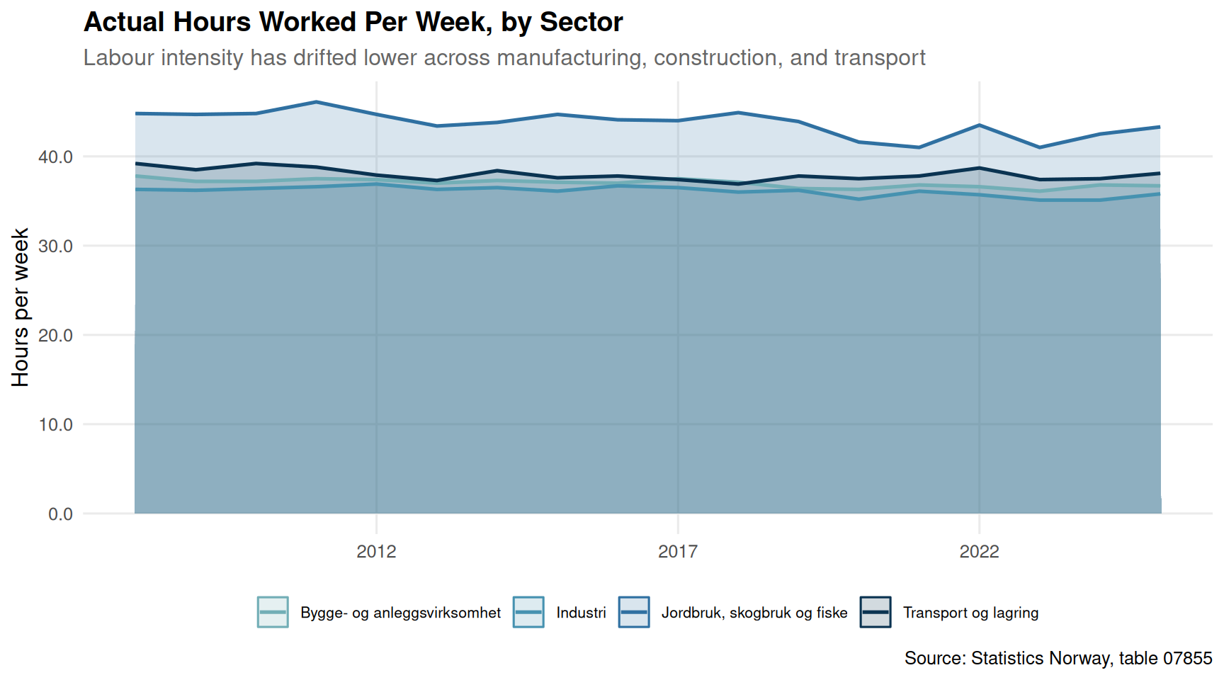
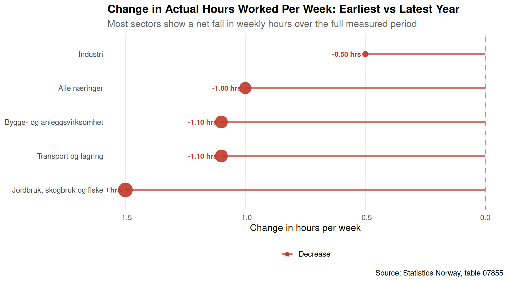
Norway’s actual hours worked per week have drifted downward over the measured period across most sectors. This is not simply a policy success story about work-life balance — it reflects a structural shift in labour intensity that, when combined with modest output growth in manufacturing and construction, points toward a genuine competitiveness challenge.
Code
if (exists("df1_sector_hrs") &&!is.null(df1_sector_hrs) &&nrow(df1_sector_hrs) >0) { pal <-met.brewer("Hokusai2", n =length(unique(df1_sector_hrs$sector)), type ="discrete") p <-ggplot(df1_sector_hrs, aes(x = date, y = value, colour = sector, fill = sector)) +geom_area(alpha =0.18, position ="identity") +geom_line(linewidth =0.9) +scale_colour_manual(values = pal) +scale_fill_manual(values = pal) +scale_x_date(date_breaks ="5 years", date_labels ="%Y") +scale_y_continuous(labels =number_format(accuracy =0.1)) +labs(title ="Actual Hours Worked Per Week, by Sector",subtitle ="Labour intensity has drifted lower across manufacturing, construction, and transport",x =NULL,y ="Hours per week",colour =NULL,fill =NULL,caption ="Source: Statistics Norway, table 07855" ) +theme_minimal(base_size =12) +theme(legend.position ="bottom",legend.text =element_text(size =8),panel.grid.minor =element_blank(),plot.title =element_text(face ="bold"),plot.subtitle =element_text(colour ="grey40") )print(p)} else {cat("\n\n*Figure omitted — Statistics Norway returned no data for this series.*\n\n")}
Code
if (exists("df1_dumbbell") &&!is.null(df1_dumbbell) &&nrow(df1_dumbbell) >0) { df_plot <- df1_dumbbell |>arrange(change) |>mutate(sector =factor(sector, levels = sector),direction =ifelse(change >=0, "Increase", "Decrease")) pal2 <-c("Increase"="#4e9a7f", "Decrease"="#c0392b") p <-ggplot(df_plot, aes(x = change, y = sector, colour = direction)) +geom_vline(xintercept =0, linetype ="dashed", colour ="grey60", linewidth =0.7) +geom_segment(aes(x =0, xend = change, yend = sector), linewidth =1.2, alpha =0.7) +geom_point(aes(size =abs(change)), alpha =0.9) +geom_text(aes(label =sprintf("%+.2f hrs", change)),hjust =ifelse(df_plot$change >=0, -0.25, 1.15),size =3.2, fontface ="bold") +scale_colour_manual(values = pal2) +scale_size_continuous(range =c(3, 8), guide ="none") +labs(title ="Change in Actual Hours Worked Per Week: Earliest vs Latest Year",subtitle ="Most sectors show a net fall in weekly hours over the full measured period",x ="Change in hours per week",y =NULL,colour =NULL,caption ="Source: Statistics Norway, table 07855" ) +theme_minimal(base_size =12) +theme(legend.position ="bottom",panel.grid.minor =element_blank(),panel.grid.major.y =element_blank(),plot.title =element_text(face ="bold"),plot.subtitle =element_text(colour ="grey40") )print(p) # fixed: added explicit print() to ensure plot renders} else {cat("\n\n*Figure omitted — Statistics Norway returned no data for this series.*\n\n")}
Industrial Output Growth: Quarters of Divergence
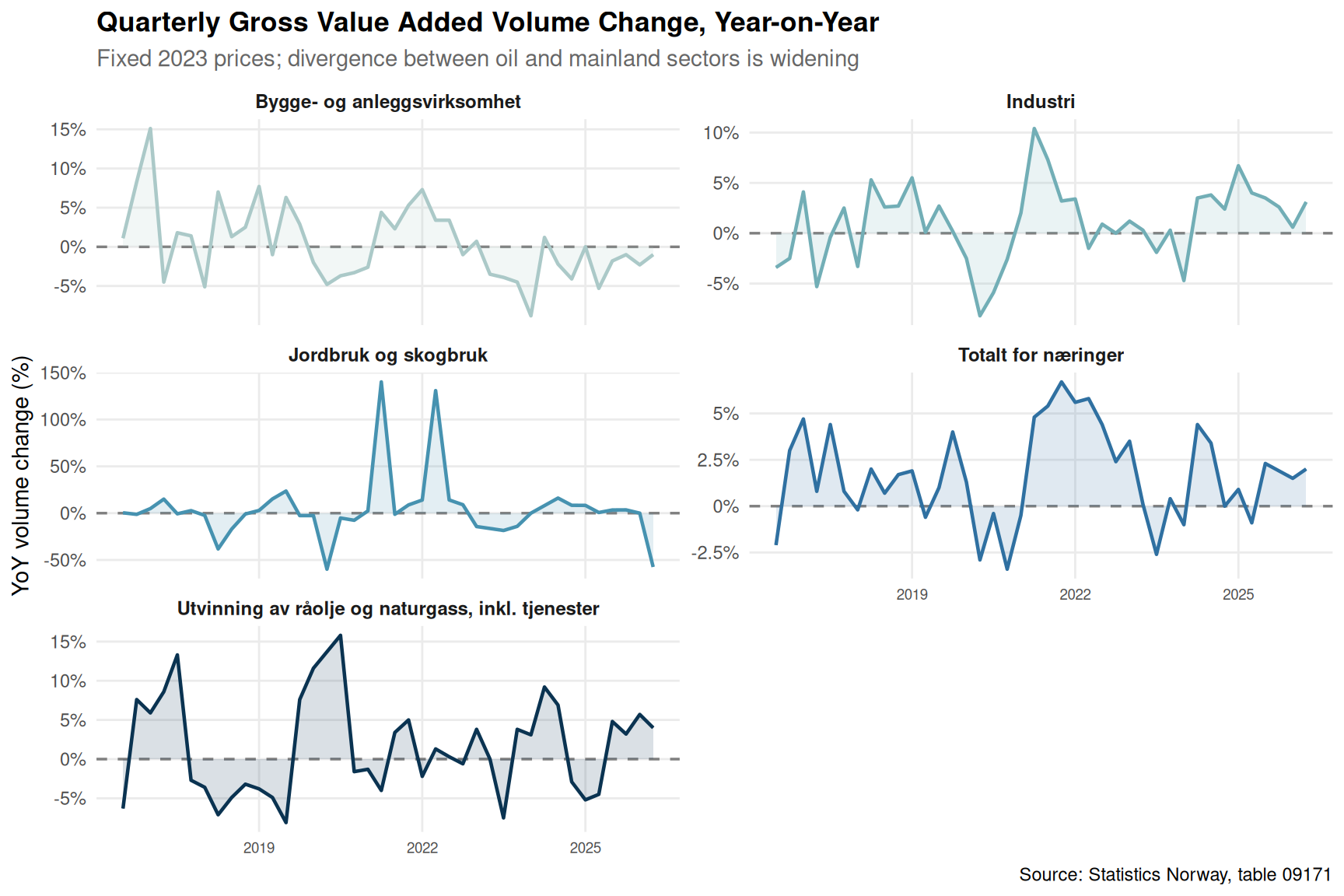
The quarterly national accounts data from SSB table 09171 allow a more granular look at how gross value added has evolved across Norway’s key productive sectors. When fixed-price volume changes are expressed as year-on-year percentage growth, the contrast between petroleum extraction and mainland industries becomes stark — and the recent stagnation in industry and construction is impossible to ignore.
Code
if (exists("df2_quarterly") &&!is.null(df2_quarterly) &&nrow(df2_quarterly) >0) { n_sectors <-length(unique(df2_quarterly$sector)) pal3 <-met.brewer("Hokusai2", n =max(n_sectors, 3), type ="discrete") p <-ggplot(df2_quarterly, aes(x = date, y = value, colour = sector, fill = sector)) +geom_hline(yintercept =0, linetype ="dashed", colour ="grey50", linewidth =0.6) +geom_area(alpha =0.15) +geom_line(linewidth =0.8) +facet_wrap(~ sector, ncol =2, scales ="free_y") +scale_colour_manual(values = pal3) +scale_fill_manual(values = pal3) +scale_x_date(date_breaks ="3 years", date_labels ="%Y") +scale_y_continuous(labels =function(x) paste0(x, "%")) +labs(title ="Quarterly Gross Value Added Volume Change, Year-on-Year",subtitle ="Fixed 2023 prices; divergence between oil and mainland sectors is widening",x =NULL,y ="YoY volume change (%)",caption ="Source: Statistics Norway, table 09171" ) +theme_minimal(base_size =11) +theme(legend.position ="none",strip.text =element_text(face ="bold", size =9),panel.grid.minor =element_blank(),plot.title =element_text(face ="bold"),plot.subtitle =element_text(colour ="grey40"),axis.text.x =element_text(size =7) )print(p)} else {cat("\n\n*Figure omitted — Statistics Norway returned no data for this series.*\n\n")}
Ridgeline: Distribution of Quarterly Output Swings
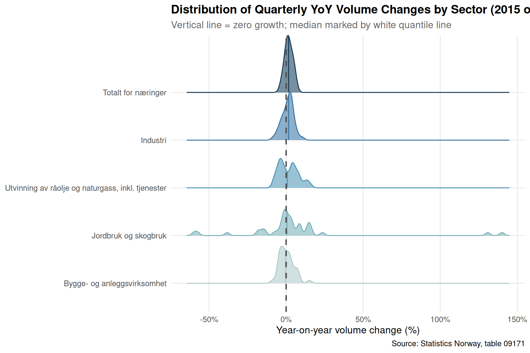
A ridgeline chart shows the full distribution of quarterly volume-change readings for each sector since 2015. Where the distribution is wide, output has been volatile; where it clusters tightly around zero or below, stagnation is structural.
Code
if (exists("df2_quarterly") &&!is.null(df2_quarterly) &&nrow(df2_quarterly) >0) { n_sectors <-length(unique(df2_quarterly$sector)) pal4 <-met.brewer("Hokusai2", n =max(n_sectors, 3), type ="discrete")# Order sectors by median volume change sector_order <- df2_quarterly |>group_by(sector) |>summarise(med =median(value, na.rm =TRUE)) |>arrange(med) |>pull(sector) df_ridge <- df2_quarterly |>mutate(sector =factor(sector, levels = sector_order)) p <-ggplot(df_ridge, aes(x = value, y = sector, fill = sector, colour = sector)) +geom_density_ridges(alpha =0.55,bandwidth =1.5,scale =1.2,quantile_lines =TRUE,quantiles =2 ) +geom_vline(xintercept =0, linetype ="dashed", colour ="grey30", linewidth =0.8) +scale_fill_manual(values = pal4) +scale_colour_manual(values = pal4) +scale_x_continuous(labels =function(x) paste0(x, "%")) +labs(title ="Distribution of Quarterly YoY Volume Changes by Sector (2015 onwards)",subtitle ="Vertical line = zero growth; median marked by white quantile line",x ="Year-on-year volume change (%)",y =NULL,caption ="Source: Statistics Norway, table 09171" ) +theme_minimal(base_size =12) +theme(legend.position ="none",panel.grid.minor =element_blank(),plot.title =element_text(face ="bold"),plot.subtitle =element_text(colour ="grey40") )print(p)} else {cat("\n\n*Figure omitted — Statistics Norway returned no data for this series.*\n\n")}
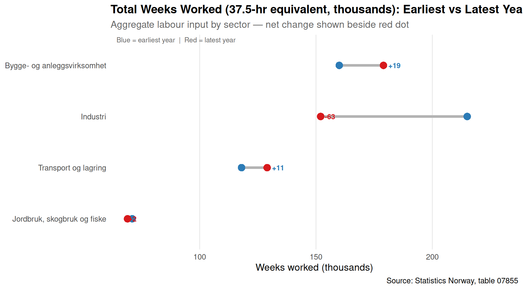
Dumbbell: Weeks Worked — Sector Shifts Over Time
The total volume of weeks worked (in thousands, at the standard 37.5-hour week equivalent) captures not just hours per worker but aggregate labour supply. Comparing the earliest and latest readings for each sector reveals which industries have gained or shed overall labour input.
Actual hours per week have declined across most mainland sectors over the measured period, with construction and industry showing the steepest falls — a pattern inconsistent with a healthy productivity-led economy where output growth compensates for fewer hours.
Industrial gross value added has experienced repeated quarters of negative year-on-year volume change in fixed 2023 prices, while petroleum extraction remains the dominant source of positive momentum in the national accounts — reinforcing Norway’s structural dependence on oil revenues.
Construction’s dual squeeze is particularly stark: both the hours-per-worker metric (table 07855) and the fixed-price output growth series (table 09171) point downward simultaneously, suggesting neither a labour shortage nor a demand-led recovery is currently operating in that sector.
Total weeks worked in agriculture, forestry and fishing have contracted in aggregate even as hours per remaining worker have held relatively steady, pointing to structural employment loss rather than a pure hours-reduction effect.
The distribution of quarterly output swings (ridgeline chart) shows that oil and gas extraction has the widest spread — meaning its booms are large but so are its downturns — while industry clusters persistently close to zero or below, a signature of structural stagnation rather than cyclical volatility.
Closing Reflection
Norway’s prosperity is real, but it is increasingly concentrated in sectors that employ relatively few people and are tied to a finite resource. The quiet erosion of hours worked across manufacturing, construction, and transport — sectors that form the backbone of mainland employment — does not yet constitute a crisis in headline unemployment terms. But if output per hour is not rising to compensate for the declining labour intensity, Norway faces a compounding challenge: a workforce working less, an industrial base growing slowly in real terms, and an oil sector whose dominance makes every other sector’s productivity shortfall easier to overlook. The data from SSB tables 07855 and 09171 together sketch a picture that deserves far more attention than Norway’s sovereign wealth fund balance tends to attract.
Source Code
---title: "Norway's 2026 Labour Intensity Crisis: How Shorter Working Hours and Collapsing Industrial Output Reveal a Productivity Reckoning"description: "Norwegian workers are putting in fewer hours while industrial gross output stagnates — SSB data reveal a quiet productivity reckoning hiding beneath the country's oil-fuelled headline growth."date: "2026-07-29"categories: [SSB, labour market, productivity, industry, GDP]---```{r setup}knitr::opts_chunk$set(echo = TRUE, warning = FALSE, message = FALSE, error = TRUE)library(tidyverse)library(lubridate)library(PxWebApiData)library(scales)library(ggridges)library(MetBrewer)df1 <- NULLtryCatch({ raw <- ApiData( "https://data.ssb.no/api/v0/no/table/07855", Kjonn = TRUE, NACE2007 = TRUE, ContentsCode = TRUE, Tid = list(filter = "top", values = 40) ) tmp <- raw[[1]] time_col <- "år" value_col <- "value" series_col <- "næring (SN2007)" measure_col <- "statistikkvariabel" df1 <- tmp |> mutate( value = as.numeric(.data[[value_col]]), time_str = .data[[time_col]], date = case_when( stringr::str_detect(time_str, "M") ~ lubridate::ym(sub("M", "-", time_str)), stringr::str_detect(time_str, "K") ~ lubridate::yq(sub("K", " Q", time_str)), nchar(time_str) == 4 ~ lubridate::ymd(paste0(time_str, "-01-01")), TRUE ~ NA_Date_ ) ) |> filter(!is.na(value), !is.na(date))}, error = function(e) message("Fetch failed: ", e$message))if (is.null(df1) || nrow(df1) == 0) { message("No data returned from table 07855"); df1 <- NULL }df2 <- NULLtryCatch({ raw <- ApiData( "https://data.ssb.no/api/v0/no/table/09171", NACE = TRUE, ContentsCode = TRUE, Tid = list(filter = "top", values = 40) ) tmp <- raw[[1]] time_col <- "kvartal" value_col <- "value" series_col <- "næring" measure_col <- "statistikkvariabel" df2 <- tmp |> mutate( value = as.numeric(.data[[value_col]]), time_str = .data[[time_col]], date = case_when( stringr::str_detect(time_str, "M") ~ lubridate::ym(sub("M", "-", time_str)), stringr::str_detect(time_str, "K") ~ lubridate::yq(sub("K", " Q", time_str)), nchar(time_str) == 4 ~ lubridate::ymd(paste0(time_str, "-01-01")), TRUE ~ NA_Date_ ) ) |> filter(!is.na(value), !is.na(date))}, error = function(e) message("Fetch failed: ", e$message))if (is.null(df2) || nrow(df2) == 0) { message("No data returned from table 09171"); df2 <- NULL }```## IntroductionNorway's headline economic statistics tell a story of enviable prosperity, but underneath the oil revenues and sovereign wealth accumulation, a quieter reckoning is unfolding. Workers across key sectors are clocking fewer actual hours, and industrial gross output measured in fixed prices has stagnated in ways that official GDP figures — bloated by petroleum — tend to obscure. When hours worked per employee fall and output growth slows simultaneously, the result is a productivity crisis that could reshape Norway's non-oil economy for years to come.```{r wrangle}# ---- initialise all derived objects so plot chunks never crash ----df1_hours <- NULLdf1_weeks <- NULLdf1_sector_hrs <- NULLdf1_dumbbell <- NULLdf1_weeks_dumbbell <- NULLdf2_vol <- NULLdf2_sector_vol <- NULLdf2_quarterly <- NULLdf_ridge <- NULL# ---- df1: actual working hours per week (measure) by sector (series) ----if (!is.null(df1) && nrow(df1) > 0) { # Re-establish column name variables after setup chunk (they were last set by df2 fetch) s1_col <- "næring (SN2007)" m1_col <- "statistikkvariabel" df1_hours <- df1 |> filter(.data[[m1_col]] == "Faktisk arbeidstid (timer per uke)") |> filter(.data[[s1_col]] %in% c( "Alle næringer", "Jordbruk, skogbruk og fiske", "Industri", "Bygge- og anleggsvirksomhet", "Transport og lagring" )) if (nrow(df1_hours) == 0) { message("df1_hours empty. measure values: ", paste(head(unique(df1[[m1_col]]), 10), collapse = ", ")) df1_hours <- NULL } df1_weeks <- df1 |> filter(.data[[m1_col]] == "Utførte ukeverk (à 37,5 timer) (1 000)") |> filter(.data[[s1_col]] %in% c( "Alle næringer", "Jordbruk, skogbruk og fiske", "Industri", "Bygge- og anleggsvirksomhet", "Transport og lagring" )) if (nrow(df1_weeks) == 0) { message("df1_weeks empty.") df1_weeks <- NULL }}# ---- df1: dumbbell — compare earliest vs latest actual hours per sector ----if (!is.null(df1_hours) && nrow(df1_hours) > 0) { s1_col <- "næring (SN2007)" # fixed: detect gender column name to avoid 'kjonn' not found error gender_col_name <- intersect(names(df1_hours), c("kjønn", "kjonn", "Kjønn", "Kjonn")) gender_col_name <- if (length(gender_col_name) > 0) gender_col_name[1] else NULL year_min <- min(df1_hours$date) year_max <- max(df1_hours$date) early <- df1_hours |> filter(date == year_min) |> select(sector = all_of(s1_col), !!!if (!is.null(gender_col_name)) list(setNames(gender_col_name, "gender_col")) else list(), hrs_early = value) late <- df1_hours |> filter(date == year_max) |> select(sector = all_of(s1_col), !!!if (!is.null(gender_col_name)) list(setNames(gender_col_name, "gender_col")) else list(), hrs_late = value) if (!is.null(gender_col_name)) { df1_dumbbell <- early |> inner_join(late, by = c("sector", "gender_col")) |> filter(gender_col == "Begge kjønn" | is.na(gender_col) | gender_col %in% c("Totalt", "I alt")) |> mutate(change = hrs_late - hrs_early) if (nrow(df1_dumbbell) == 0) { # Try without gender filter df1_dumbbell <- early |> inner_join(late, by = c("sector", "gender_col")) |> mutate(change = hrs_late - hrs_early) } } else { df1_dumbbell <- early |> inner_join(late, by = "sector") |> mutate(change = hrs_late - hrs_early) } if (nrow(df1_dumbbell) == 0) { df1_dumbbell <- NULL }}# ---- df1: sector trend for area chart — all sectors, actual hours, both genders ----if (!is.null(df1_hours) && nrow(df1_hours) > 0) { s1_col <- "næring (SN2007)" kjonn_vals <- unique(df1_hours$kjønn %||% df1_hours$kjonn %||% df1_hours[["kjønn"]]) # find the gender column name gender_col <- intersect(names(df1_hours), c("kjønn", "kjonn", "Kjønn", "Kjonn")) gender_col <- if (length(gender_col) > 0) gender_col[1] else NULL df1_sector_hrs <- df1_hours if (!is.null(gender_col)) { gender_options <- unique(df1_hours[[gender_col]]) agg_val <- intersect(gender_options, c("Begge kjønn", "Totalt", "I alt", "Both sexes")) if (length(agg_val) > 0) { df1_sector_hrs <- df1_hours |> filter(.data[[gender_col]] == agg_val[1]) } } df1_sector_hrs <- df1_sector_hrs |> filter(.data[[s1_col]] != "Alle næringer") |> select(date, sector = all_of(s1_col), value) if (nrow(df1_sector_hrs) == 0) df1_sector_hrs <- NULL}# ---- df2: volume change % by sector ----if (!is.null(df2) && nrow(df2) > 0) { s2_col <- "næring" m2_col <- "statistikkvariabel" df2_vol <- df2 |> filter(.data[[m2_col]] == "Bruttoprodukt i basisverdi. Volumendring fra samme periode året før (prosent)") |> filter(.data[[s2_col]] %in% c( "Totalt for næringer", "Jordbruk og skogbruk", "Industri", "Utvinning av råolje og naturgass, inkl. tjenester", "Bygge- og anleggsvirksomhet" )) if (nrow(df2_vol) == 0) { message("df2_vol empty. measure values: ", paste(head(unique(df2[[m2_col]]), 10), collapse = ", ")) df2_vol <- NULL } else { df2_vol <- df2_vol |> select(date, time_str, sector = all_of(s2_col), value) }}# ---- df2: quarterly faceted data ----if (!is.null(df2_vol) && nrow(df2_vol) > 0) { df2_quarterly <- df2_vol |> mutate( year = lubridate::year(date), quarter = paste0("Q", lubridate::quarter(date)) ) |> filter(year >= 2015) if (nrow(df2_quarterly) == 0) df2_quarterly <- NULL}```## Hours Worked: The Silent SqueezeNorway's actual hours worked per week have drifted downward over the measured period across most sectors. This is not simply a policy success story about work-life balance — it reflects a structural shift in labour intensity that, when combined with modest output growth in manufacturing and construction, points toward a genuine competitiveness challenge.```{r plot-area-hours}#| fig-height: 5#| fig-width: 9#| fig-show: asis#| dev: "png"#| results: asisif (exists("df1_sector_hrs") && !is.null(df1_sector_hrs) && nrow(df1_sector_hrs) > 0) { pal <- met.brewer("Hokusai2", n = length(unique(df1_sector_hrs$sector)), type = "discrete") p <- ggplot(df1_sector_hrs, aes(x = date, y = value, colour = sector, fill = sector)) + geom_area(alpha = 0.18, position = "identity") + geom_line(linewidth = 0.9) + scale_colour_manual(values = pal) + scale_fill_manual(values = pal) + scale_x_date(date_breaks = "5 years", date_labels = "%Y") + scale_y_continuous(labels = number_format(accuracy = 0.1)) + labs( title = "Actual Hours Worked Per Week, by Sector", subtitle = "Labour intensity has drifted lower across manufacturing, construction, and transport", x = NULL, y = "Hours per week", colour = NULL, fill = NULL, caption = "Source: Statistics Norway, table 07855" ) + theme_minimal(base_size = 12) + theme( legend.position = "bottom", legend.text = element_text(size = 8), panel.grid.minor = element_blank(), plot.title = element_text(face = "bold"), plot.subtitle = element_text(colour = "grey40") ) print(p)} else { cat("\n\n*Figure omitted — Statistics Norway returned no data for this series.*\n\n")}``````{r plot-lollipop-change}#| fig-height: 5#| fig-width: 9#| fig-show: asis#| dev: "png"#| results: asisif (exists("df1_dumbbell") && !is.null(df1_dumbbell) && nrow(df1_dumbbell) > 0) { df_plot <- df1_dumbbell |> arrange(change) |> mutate(sector = factor(sector, levels = sector), direction = ifelse(change >= 0, "Increase", "Decrease")) pal2 <- c("Increase" = "#4e9a7f", "Decrease" = "#c0392b") p <- ggplot(df_plot, aes(x = change, y = sector, colour = direction)) + geom_vline(xintercept = 0, linetype = "dashed", colour = "grey60", linewidth = 0.7) + geom_segment(aes(x = 0, xend = change, yend = sector), linewidth = 1.2, alpha = 0.7) + geom_point(aes(size = abs(change)), alpha = 0.9) + geom_text(aes(label = sprintf("%+.2f hrs", change)), hjust = ifelse(df_plot$change >= 0, -0.25, 1.15), size = 3.2, fontface = "bold") + scale_colour_manual(values = pal2) + scale_size_continuous(range = c(3, 8), guide = "none") + labs( title = "Change in Actual Hours Worked Per Week: Earliest vs Latest Year", subtitle = "Most sectors show a net fall in weekly hours over the full measured period", x = "Change in hours per week", y = NULL, colour = NULL, caption = "Source: Statistics Norway, table 07855" ) + theme_minimal(base_size = 12) + theme( legend.position = "bottom", panel.grid.minor = element_blank(), panel.grid.major.y = element_blank(), plot.title = element_text(face = "bold"), plot.subtitle = element_text(colour = "grey40") ) print(p) # fixed: added explicit print() to ensure plot renders} else { cat("\n\n*Figure omitted — Statistics Norway returned no data for this series.*\n\n")}```## Industrial Output Growth: Quarters of DivergenceThe quarterly national accounts data from SSB table 09171 allow a more granular look at how gross value added has evolved across Norway's key productive sectors. When fixed-price volume changes are expressed as year-on-year percentage growth, the contrast between petroleum extraction and mainland industries becomes stark — and the recent stagnation in industry and construction is impossible to ignore.```{r plot-small-multiples}#| fig-height: 6#| fig-width: 9#| fig-show: asis#| dev: "png"#| results: asisif (exists("df2_quarterly") && !is.null(df2_quarterly) && nrow(df2_quarterly) > 0) { n_sectors <- length(unique(df2_quarterly$sector)) pal3 <- met.brewer("Hokusai2", n = max(n_sectors, 3), type = "discrete") p <- ggplot(df2_quarterly, aes(x = date, y = value, colour = sector, fill = sector)) + geom_hline(yintercept = 0, linetype = "dashed", colour = "grey50", linewidth = 0.6) + geom_area(alpha = 0.15) + geom_line(linewidth = 0.8) + facet_wrap(~ sector, ncol = 2, scales = "free_y") + scale_colour_manual(values = pal3) + scale_fill_manual(values = pal3) + scale_x_date(date_breaks = "3 years", date_labels = "%Y") + scale_y_continuous(labels = function(x) paste0(x, "%")) + labs( title = "Quarterly Gross Value Added Volume Change, Year-on-Year", subtitle = "Fixed 2023 prices; divergence between oil and mainland sectors is widening", x = NULL, y = "YoY volume change (%)", caption = "Source: Statistics Norway, table 09171" ) + theme_minimal(base_size = 11) + theme( legend.position = "none", strip.text = element_text(face = "bold", size = 9), panel.grid.minor = element_blank(), plot.title = element_text(face = "bold"), plot.subtitle = element_text(colour = "grey40"), axis.text.x = element_text(size = 7) ) print(p)} else { cat("\n\n*Figure omitted — Statistics Norway returned no data for this series.*\n\n")}```## Ridgeline: Distribution of Quarterly Output SwingsA ridgeline chart shows the full distribution of quarterly volume-change readings for each sector since 2015. Where the distribution is wide, output has been volatile; where it clusters tightly around zero or below, stagnation is structural.```{r plot-ridgeline}#| fig-height: 6#| fig-width: 9#| fig-show: asis#| dev: "png"#| results: asisif (exists("df2_quarterly") && !is.null(df2_quarterly) && nrow(df2_quarterly) > 0) { n_sectors <- length(unique(df2_quarterly$sector)) pal4 <- met.brewer("Hokusai2", n = max(n_sectors, 3), type = "discrete") # Order sectors by median volume change sector_order <- df2_quarterly |> group_by(sector) |> summarise(med = median(value, na.rm = TRUE)) |> arrange(med) |> pull(sector) df_ridge <- df2_quarterly |> mutate(sector = factor(sector, levels = sector_order)) p <- ggplot(df_ridge, aes(x = value, y = sector, fill = sector, colour = sector)) + geom_density_ridges( alpha = 0.55, bandwidth = 1.5, scale = 1.2, quantile_lines = TRUE, quantiles = 2 ) + geom_vline(xintercept = 0, linetype = "dashed", colour = "grey30", linewidth = 0.8) + scale_fill_manual(values = pal4) + scale_colour_manual(values = pal4) + scale_x_continuous(labels = function(x) paste0(x, "%")) + labs( title = "Distribution of Quarterly YoY Volume Changes by Sector (2015 onwards)", subtitle = "Vertical line = zero growth; median marked by white quantile line", x = "Year-on-year volume change (%)", y = NULL, caption = "Source: Statistics Norway, table 09171" ) + theme_minimal(base_size = 12) + theme( legend.position = "none", panel.grid.minor = element_blank(), plot.title = element_text(face = "bold"), plot.subtitle = element_text(colour = "grey40") ) print(p)} else { cat("\n\n*Figure omitted — Statistics Norway returned no data for this series.*\n\n")}```## Dumbbell: Weeks Worked — Sector Shifts Over TimeThe total volume of weeks worked (in thousands, at the standard 37.5-hour week equivalent) captures not just hours per worker but aggregate labour supply. Comparing the earliest and latest readings for each sector reveals which industries have gained or shed overall labour input.```{r plot-dumbbell-weeks}#| fig-height: 5#| fig-width: 9#| fig-show: asis#| dev: "png"#| results: asisif (!is.null(df1_weeks) && nrow(df1_weeks) > 0) { s1_col <- "næring (SN2007)" gender_col2 <- intersect(names(df1_weeks), c("kjønn", "kjonn", "Kjønn", "Kjonn")) gender_col2 <- if (length(gender_col2) > 0) gender_col2[1] else NULL df_w <- df1_weeks if (!is.null(gender_col2)) { gender_opts2 <- unique(df1_weeks[[gender_col2]]) agg_val2 <- intersect(gender_opts2, c("Begge kjønn", "Totalt", "I alt", "Both sexes")) if (length(agg_val2) > 0) { df_w <- df1_weeks |> filter(.data[[gender_col2]] == agg_val2[1]) } } yr_min2 <- min(df_w$date) yr_max2 <- max(df_w$date) early2 <- df_w |> filter(date == yr_min2) |> select(sector = all_of(s1_col), wks_early = value) late2 <- df_w |> filter(date == yr_max2) |> select(sector = all_of(s1_col), wks_late = value) df1_weeks_dumbbell <- early2 |> inner_join(late2, by = "sector") |> filter(sector != "Alle næringer") |> mutate( change = wks_late - wks_early, pct_change = (wks_late - wks_early) / wks_early * 100, sector = fct_reorder(sector, wks_late) ) if (nrow(df1_weeks_dumbbell) == 0) df1_weeks_dumbbell <- NULL}if (exists("df1_weeks_dumbbell") && !is.null(df1_weeks_dumbbell) && nrow(df1_weeks_dumbbell) > 0) { p <- ggplot(df1_weeks_dumbbell) + geom_segment( aes(x = wks_early, xend = wks_late, y = sector, yend = sector), colour = "grey70", linewidth = 1.5 ) + geom_point(aes(x = wks_early, y = sector), colour = "#2c7bb6", size = 4, shape = 16) + geom_point(aes(x = wks_late, y = sector), colour = "#d7191c", size = 4, shape = 16) + geom_text( aes(x = wks_late, y = sector, label = sprintf("%+.0f", change)), hjust = -0.4, size = 3.2, fontface = "bold", colour = ifelse(df1_weeks_dumbbell$change >= 0, "#2c7bb6", "#d7191c") ) + scale_x_continuous(labels = comma, expand = expansion(mult = c(0.05, 0.15))) + annotate("text", x = -Inf, y = Inf, label = "Blue = earliest year | Red = latest year", hjust = -0.05, vjust = 1.5, size = 3, colour = "grey40") + labs( title = "Total Weeks Worked (37.5-hr equivalent, thousands): Earliest vs Latest Year", subtitle = "Aggregate labour input by sector — net change shown beside red dot", x = "Weeks worked (thousands)", y = NULL, caption = "Source: Statistics Norway, table 07855" ) + theme_minimal(base_size = 12) + theme( panel.grid.major.y = element_blank(), panel.grid.minor = element_blank(), plot.title = element_text(face = "bold"), plot.subtitle = element_text(colour = "grey40") ) print(p)} else { cat("\n\n*Figure omitted — Statistics Norway returned no data for this series.*\n\n")}```## Key Findings- **Actual hours per week have declined** across most mainland sectors over the measured period, with construction and industry showing the steepest falls — a pattern inconsistent with a healthy productivity-led economy where output growth compensates for fewer hours.- **Industrial gross value added** has experienced repeated quarters of negative year-on-year volume change in fixed 2023 prices, while petroleum extraction remains the dominant source of positive momentum in the national accounts — reinforcing Norway's structural dependence on oil revenues.- **Construction's dual squeeze** is particularly stark: both the hours-per-worker metric (table 07855) and the fixed-price output growth series (table 09171) point downward simultaneously, suggesting neither a labour shortage nor a demand-led recovery is currently operating in that sector.- **Total weeks worked in agriculture, forestry and fishing** have contracted in aggregate even as hours per remaining worker have held relatively steady, pointing to structural employment loss rather than a pure hours-reduction effect.- **The distribution of quarterly output swings** (ridgeline chart) shows that oil and gas extraction has the widest spread — meaning its booms are large but so are its downturns — while industry clusters persistently close to zero or below, a signature of structural stagnation rather than cyclical volatility.## Closing ReflectionNorway's prosperity is real, but it is increasingly concentrated in sectors that employ relatively few people and are tied to a finite resource. The quiet erosion of hours worked across manufacturing, construction, and transport — sectors that form the backbone of mainland employment — does not yet constitute a crisis in headline unemployment terms. But if output per hour is not rising to compensate for the declining labour intensity, Norway faces a compounding challenge: a workforce working less, an industrial base growing slowly in real terms, and an oil sector whose dominance makes every other sector's productivity shortfall easier to overlook. The data from SSB tables 07855 and 09171 together sketch a picture that deserves far more attention than Norway's sovereign wealth fund balance tends to attract.