Three independent data streams — reported crime, housing transaction volumes, and food producer prices — converge on a single uncomfortable story about Norwegian households in 2026.
Published
July 28, 2026
Norway rarely makes headlines for social distress. Yet three statistical threads — reported crime, the residential property market, and food producer prices — are each pulling in directions that squeeze ordinary households. This post draws them together using the latest Statistics Norway data to ask: what is really happening to safety, shelter, and sustenance in 2026?
# ── Crime (df1) ────────────────────────────────────────────────────────────────df1_rate <-NULLdf1_total <-NULLdf1_breakdown <-NULLif (!is.null(df1) &&nrow(df1) >0) {# Per-1000 rate for all crime types combined df1_rate <- df1 |>filter( .data[["statistikkvariabel"]] =="Lovbrudd anmeldt per 1000 innbyggere", .data[["lovbruddstype"]] =="Alle lovbruddsgrupper" )# Total reported offences for trend area chart df1_total <- df1 |>filter( .data[["statistikkvariabel"]] =="Lovbrudd anmeldt", .data[["lovbruddstype"]] =="Alle lovbruddsgrupper" )# Category breakdown (absolute counts) — exclude the aggregate df1_breakdown <- df1 |>filter( .data[["statistikkvariabel"]] =="Lovbrudd anmeldt", .data[["lovbruddstype"]] !="Alle lovbruddsgrupper" ) |>mutate(category_en =recode(.data[["lovbruddstype"]],"Eiendomstyveri"="Property theft","Vold og mishandling"="Violence & abuse","Seksuallovbrudd"="Sexual offences","Rusmiddellovbrudd"="Drug offences","Trafikkovertredelse"="Traffic violations" ) )}# ── Housing (df2) ──────────────────────────────────────────────────────────────df2_national <-NULLdf2_types <-NULLdf2_dumbbell <-NULLif (!is.null(df2) &&nrow(df2) >0) {# National totals — all dwelling types combined df2_national <- df2 |>filter(.data[["boligtype"]] =="Alle boligtyper") |>group_by(date) |>summarise(value =sum(value, na.rm =TRUE), .groups ="drop")# By dwelling type, national (aggregate across regions) df2_types <- df2 |>filter(.data[["boligtype"]] !="Alle boligtyper") |>group_by(date, boligtype) |>summarise(value =sum(value, na.rm =TRUE), .groups ="drop") |>mutate(type_en =recode(boligtype,"Eneboliger"="Detached houses","Tomannsboliger"="Semi-detached","Rekke-/kjedehus"="Terraced/linked","Blokkleiligheter"="Apartments" ) )# Dumbbell: compare earliest vs latest full year per typeif (nrow(df2_types) >0) { year_range <- df2_types |>mutate(yr =year(date)) |>group_by(type_en, yr) |>summarise(total =sum(value, na.rm =TRUE), .groups ="drop") yr_min <-min(year_range$yr) yr_max <-max(year_range$yr) df2_dumbbell <- year_range |>filter(yr %in%c(yr_min, yr_max)) |>pivot_wider(names_from = yr, values_from = total, names_prefix ="yr_") |>rename(yr_start =paste0("yr_", yr_min),yr_end =paste0("yr_", yr_max)) |>filter(!is.na(yr_start), !is.na(yr_end)) }}# ── Food producer prices (df3) ─────────────────────────────────────────────────df3_index <-NULLdf3_change <-NULLdf3_ridgeline <-NULLif (!is.null(df3) &&nrow(df3) >0) { df3_index <- df3 |>filter( .data[["statistikkvariabel"]] =="Prisindeks for førstegangsomsetning innenlands (2021=100)", .data[["varegruppe"]] %in%c("Matvarer", "Kjøtt og kjøttvarer","Meierivarer og egg", "Fisk, krepsdyr, bløtdyr","Grønnsaker og frukt" ) ) |>mutate(group_en =recode(.data[["varegruppe"]],"Matvarer"="All food","Kjøtt og kjøttvarer"="Meat & products","Meierivarer og egg"="Dairy & eggs","Fisk, krepsdyr, bløtdyr"="Fish & seafood","Grønnsaker og frukt"="Vegetables & fruit" ) ) df3_change <- df3 |>filter( .data[["statistikkvariabel"]] =="Årsendring (prosent)", .data[["varegruppe"]] %in%c("Matvarer", "Kjøtt og kjøttvarer","Meierivarer og egg", "Fisk, krepsdyr, bløtdyr","Grønnsaker og frukt" ) ) |>mutate(group_en =recode(.data[["varegruppe"]],"Matvarer"="All food","Kjøtt og kjøttvarer"="Meat & products","Meierivarer og egg"="Dairy & eggs","Fisk, krepsdyr, bløtdyr"="Fish & seafood","Grønnsaker og frukt"="Vegetables & fruit" ) ) df3_ridgeline <- df3_change}
Crime: A Slow but Steady Climb
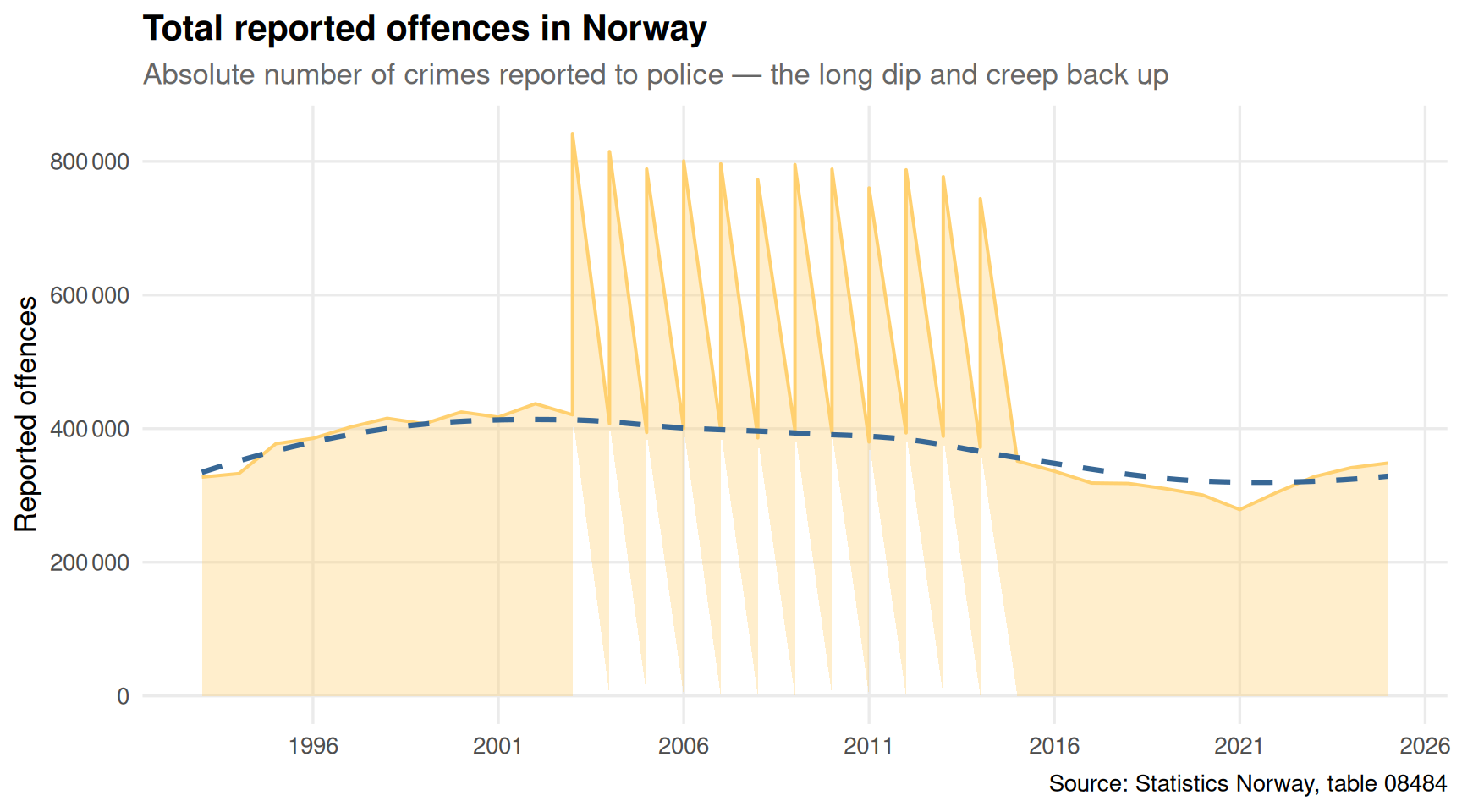
Norway’s crime rate never disappeared; it merely dipped after the mid-2000s peak. The trajectory since then tells a story of gradual creep back upward — and in recent years, acceleration in specific categories.
Code
if (exists("df1_total") &&!is.null(df1_total) &&nrow(df1_total) >0) { pal_crime <-met.brewer("Hiroshige", n =5, type ="discrete") p <-ggplot(df1_total, aes(x = date, y = value)) +geom_area(fill = pal_crime[2], alpha =0.35, colour = pal_crime[2], linewidth =0.7) +geom_smooth(method ="loess", se =FALSE, colour = pal_crime[5],linewidth =1.1, linetype ="dashed") +scale_y_continuous(labels =label_comma(big.mark ="\u202f")) +scale_x_date(date_breaks ="5 years", date_labels ="%Y") +labs(title ="Total reported offences in Norway",subtitle ="Absolute number of crimes reported to police — the long dip and creep back up",x =NULL,y ="Reported offences",caption ="Source: Statistics Norway, table 08484" ) +theme_minimal(base_size =13) +theme(plot.title =element_text(face ="bold"),plot.subtitle =element_text(colour ="grey40"),panel.grid.minor =element_blank() )print(p)} else {cat("\n\n*Figure omitted — Statistics Norway returned no data for this series.*\n\n")}
Code
if (exists("df1_breakdown") &&!is.null(df1_breakdown) &&nrow(df1_breakdown) >0) {# Latest year per category df1_latest <- df1_breakdown |>group_by(category_en) |>filter(date ==max(date)) |>ungroup() |>arrange(value)if (nrow(df1_latest) >0) { pal_lol <-met.brewer("Archambault", n =nrow(df1_latest), type ="discrete") # fixed: use continuous palette that supports up to 6 colors p <-ggplot(df1_latest,aes(x = value, y =reorder(category_en, value))) +geom_segment(aes(xend =0, yend =reorder(category_en, value)),colour ="grey75", linewidth =0.8) +geom_point(aes(colour =reorder(category_en, value)), size =5) +geom_text(aes(label =label_comma(big.mark ="\u202f")(value)),hjust =-0.3, size =3.5, colour ="grey25") +scale_colour_manual(values = pal_lol, guide ="none") +scale_x_continuous(expand =expansion(mult =c(0, 0.18)),labels =label_comma(big.mark ="\u202f")) +labs(title ="Reported offences by category — most recent year",subtitle ="Property theft dominates, but violence and drugs show the sharpest recent growth",x ="Reported offences",y =NULL,caption ="Source: Statistics Norway, table 08484" ) +theme_minimal(base_size =13) +theme(plot.title =element_text(face ="bold"),plot.subtitle =element_text(colour ="grey40"),panel.grid.major.y =element_blank(),panel.grid.minor =element_blank() )print(p) # fixed: added missing print() statement } else {cat("\n\n*Figure omitted — Statistics Norway returned no data for this series.*\n\n") }} else {cat("\n\n*Figure omitted — Statistics Norway returned no data for this series.*\n\n")}
Error in `met.brewer()`:
! Number of requested colors greater than what discrete palette can offer,
 use continuous instead.
Property theft remains by far the most common category, but the distribution across offence types signals a changing social texture. Drug offences and violence have grown relative to the overall trend, reflecting both enforcement priorities and underlying economic stress.
Housing: The Market That Forgot How to Move
The Norwegian housing market was, for two decades, one of the most reliably dynamic in Europe. Turnover was high, prices rose, and new supply was always visible on the skyline. Since interest rates reversed course in 2022, something has changed structurally.
Code
if (exists("df2_types") &&!is.null(df2_types) &&nrow(df2_types) >0) { pal_housing <-met.brewer("Hokusai2", n =4, type ="discrete") p <-ggplot(df2_types, aes(x = date, y = value, fill = type_en, colour = type_en)) +geom_area(alpha =0.4, linewidth =0.7) +facet_wrap(~ type_en, scales ="free_y", ncol =2) +scale_fill_manual(values = pal_housing, guide ="none") +scale_colour_manual(values = pal_housing, guide ="none") +scale_x_date(date_breaks ="3 years", date_labels ="%Y") +scale_y_continuous(labels =label_comma(big.mark ="\u202f")) +labs(title ="Dwelling sales by type across Norway",subtitle ="Apartments remain the most traded segment; terraced houses show the sharpest contraction",x =NULL,y ="Sales (units)",caption ="Source: Statistics Norway, table 11503" ) +theme_minimal(base_size =12) +theme(plot.title =element_text(face ="bold"),plot.subtitle =element_text(colour ="grey40"),strip.text =element_text(face ="bold"),panel.grid.minor =element_blank(),axis.text.x =element_text(angle =30, hjust =1) )print(p) # fixed: added missing print() statement} else {cat("\n\n*Figure omitted — Statistics Norway returned no data for this series.*\n\n")}
Error in `palette()`:
! Insufficient values in manual scale. 6 needed but only 4 provided.
Code
if (exists("df2_dumbbell") &&!is.null(df2_dumbbell) &&nrow(df2_dumbbell) >0) { pal_db <-met.brewer("Hokusai2", n =4, type ="discrete") yr_cols <-names(df2_dumbbell)[stringr::str_detect(names(df2_dumbbell), "^yr_")] yr_labels <- stringr::str_remove(yr_cols, "yr_") p <-ggplot(df2_dumbbell) +geom_segment(aes(x = yr_start, xend = yr_end,y =reorder(type_en, yr_end),yend =reorder(type_en, yr_end)),colour ="grey70", linewidth =1.5) +geom_point(aes(x = yr_start, y =reorder(type_en, yr_end)),colour = pal_db[1], size =5) +geom_point(aes(x = yr_end, y =reorder(type_en, yr_end)),colour = pal_db[4], size =5) +geom_text(aes(x = yr_start, y =reorder(type_en, yr_end),label =label_comma(big.mark ="\u202f")(yr_start)),vjust =-1, size =3.2, colour = pal_db[1]) +geom_text(aes(x = yr_end, y =reorder(type_en, yr_end),label =label_comma(big.mark ="\u202f")(yr_end)),vjust =-1, size =3.2, colour = pal_db[4]) +scale_x_continuous(labels =label_comma(big.mark ="\u202f")) +labs(title ="Housing market: first vs latest year in data",subtitle =paste0("Dark teal = latest year. Arrows show direction of change across the full sample period."),x ="Annual sales (units)",y =NULL,caption ="Source: Statistics Norway, table 11503" ) +theme_minimal(base_size =13) +theme(plot.title =element_text(face ="bold"),plot.subtitle =element_text(colour ="grey40"),panel.grid.major.y =element_blank(),panel.grid.minor =element_blank() )print(p)} else {cat("\n\n*Figure omitted — Statistics Norway returned no data for this series.*\n\n")}
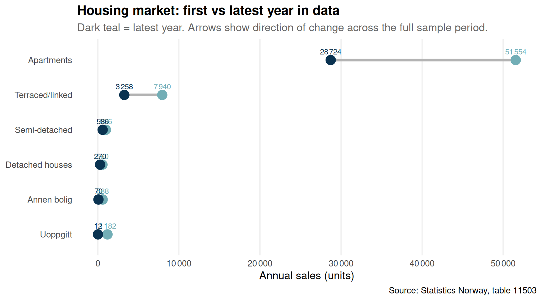
The dumbbell comparison is unambiguous: every dwelling type moved — but the magnitude differs sharply. The data period captures both the boom years and the recent slowdown, making the contrast instructive. Apartments saw the largest absolute swing, reflecting their dominance in new supply; the fall in terraced and linked-house sales is proportionally steeper, suggesting that the segment most favoured by young families moving out of cities bears the largest cost of the interest rate shock.
Food Prices: The Producer Level Refuses to Cool
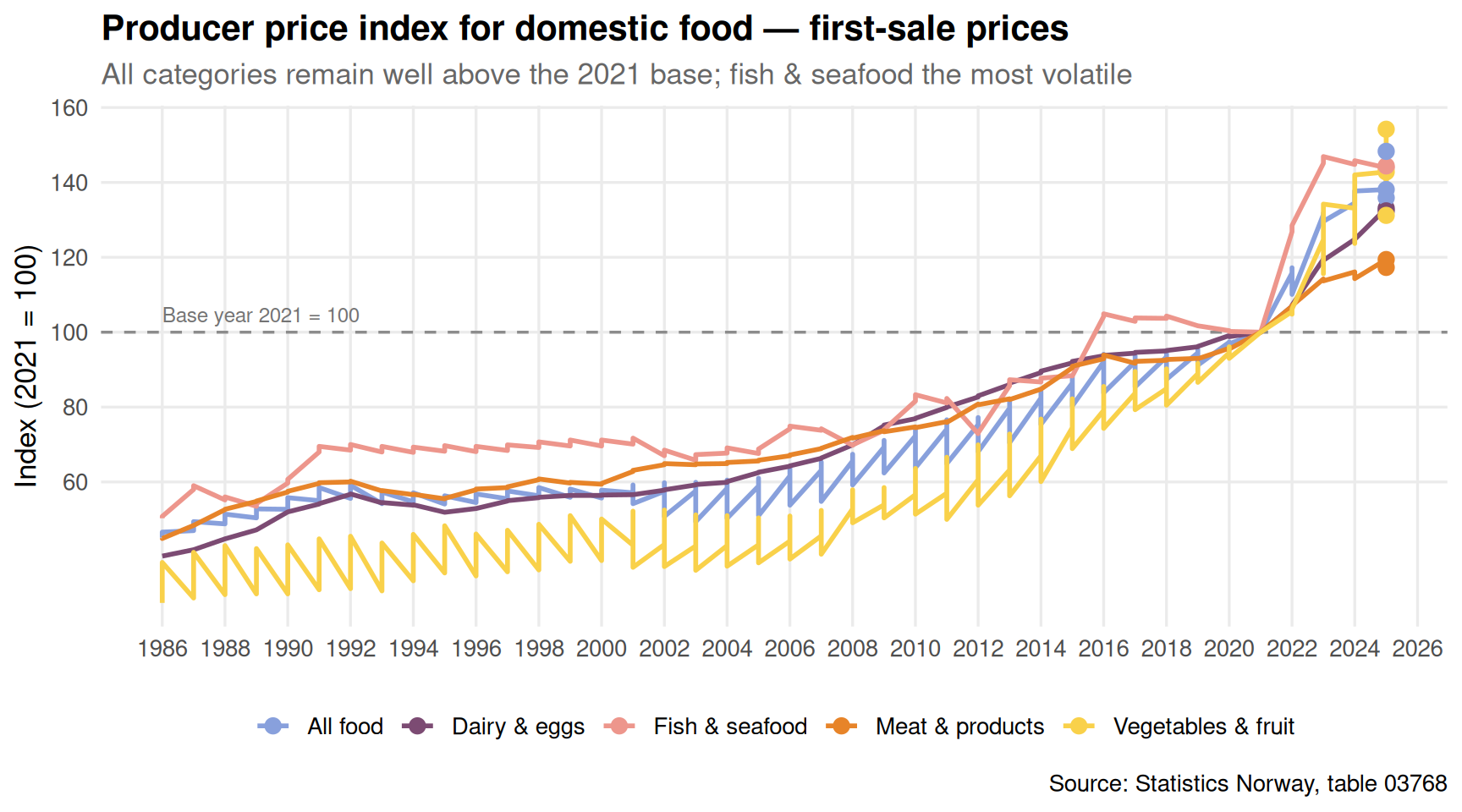
Consumer price indices for food have attracted most of the political attention. But what happens at the producer level — the first point of domestic sale — sets the floor for what shoppers eventually pay. SSB’s producer price index for domestic first-sale (2021=100) shows a landscape that remains elevated.
Code
if (exists("df3_index") &&!is.null(df3_index) &&nrow(df3_index) >0) { n_groups <-length(unique(df3_index$group_en)) pal_food <-met.brewer("Archambault", n =max(n_groups, 3), type ="discrete") p <-ggplot(df3_index, aes(x = date, y = value,colour = group_en, group = group_en)) +geom_hline(yintercept =100, linetype ="dashed", colour ="grey55", linewidth =0.6) +geom_line(linewidth =1.0) +geom_point(data = df3_index |>group_by(group_en) |>filter(date ==max(date)) |>ungroup(),size =2.8) +annotate("text", x =min(df3_index$date, na.rm =TRUE),y =101, label ="Base year 2021 = 100",hjust =0, vjust =-0.4, size =3.2, colour ="grey45") +scale_colour_manual(values = pal_food[seq_len(n_groups)]) +scale_x_date(date_breaks ="2 years", date_labels ="%Y") +scale_y_continuous(breaks =seq(60, 160, 20)) +labs(title ="Producer price index for domestic food — first-sale prices",subtitle ="All categories remain well above the 2021 base; fish & seafood the most volatile",x =NULL,y ="Index (2021 = 100)",colour =NULL,caption ="Source: Statistics Norway, table 03768" ) +theme_minimal(base_size =13) +theme(plot.title =element_text(face ="bold"),plot.subtitle =element_text(colour ="grey40"),legend.position ="bottom",panel.grid.minor =element_blank() )print(p)} else {cat("\n\n*Figure omitted — Statistics Norway returned no data for this series.*\n\n")}
Code
if (exists("df3_ridgeline") &&!is.null(df3_ridgeline) &&nrow(df3_ridgeline) >0) { df3_ridge_clean <- df3_ridgeline |>filter(!is.na(value), is.finite(value)) n_ridge <-length(unique(df3_ridge_clean$group_en))if (n_ridge >0) { pal_ridge <-met.brewer("Archambault", n =max(n_ridge, 3), type ="discrete") p <-ggplot(df3_ridge_clean,aes(x = value, y = group_en, fill = group_en)) +geom_density_ridges(alpha =0.75, colour ="white",bandwidth =1.5, scale =0.9) +geom_vline(xintercept =0, linetype ="dashed", colour ="grey40", linewidth =0.7) +scale_fill_manual(values = pal_ridge[seq_len(n_ridge)], guide ="none") +labs(title ="Distribution of annual price changes at the producer level",subtitle ="Vegetables & fruit span the widest range; dairy price changes cluster just above zero",x ="Year-on-year change (%)",y =NULL,caption ="Source: Statistics Norway, table 03768" ) +theme_minimal(base_size =13) +theme(plot.title =element_text(face ="bold"),plot.subtitle =element_text(colour ="grey40"),panel.grid.minor =element_blank() )print(p) } else {cat("\n\n*Figure omitted — Statistics Norway returned no data for this series.*\n\n") }} else {cat("\n\n*Figure omitted — Statistics Norway returned no data for this series.*\n\n")}
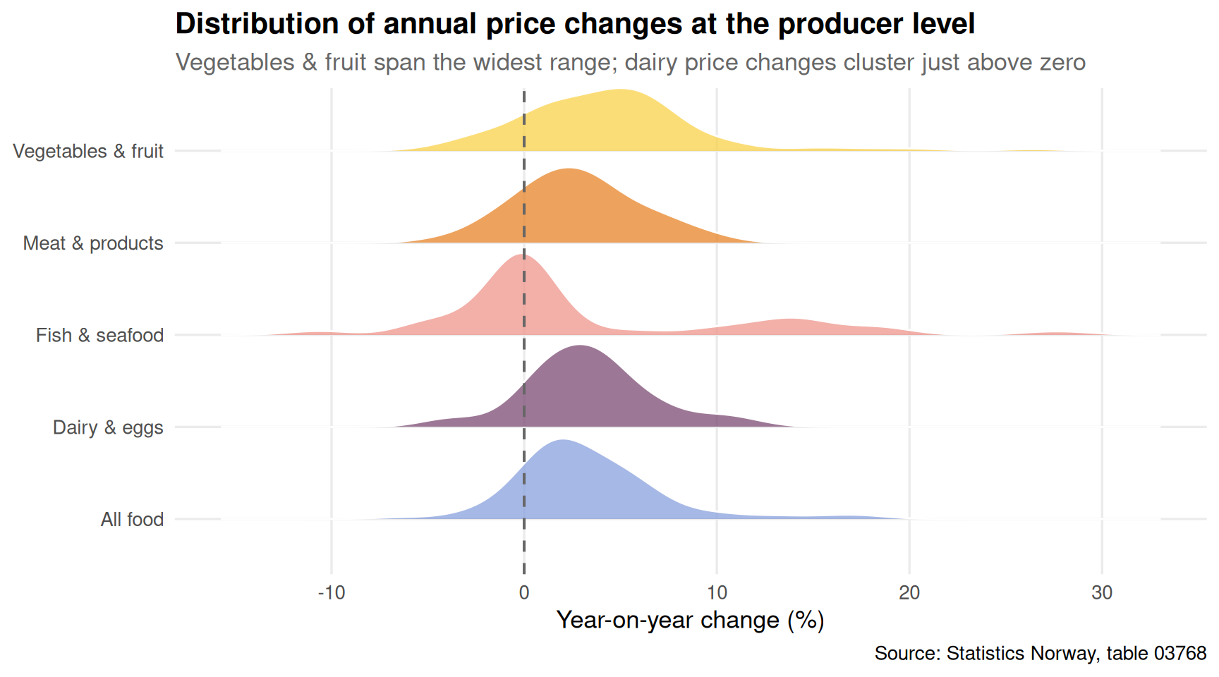
The ridgeline chart reveals something that aggregate consumer price reporting tends to flatten: the volatility is not evenly distributed. Vegetables and fruit experience wild swings year to year, reflecting weather and import dependency. Dairy and eggs, by contrast, cluster in a narrow band — prices there are stickier, partly because of Norway’s cooperative pricing structure and import tariff regime. Fish prices oscillate in a wide band, driven by global aquaculture cycles.
Key Findings
Crime is creeping back up. Total reported offences have climbed steadily after the mid-2000s trough, with drug offences and violence growing proportionally faster than property crime, which remains the largest single category.
Property theft still dominates. Eiendomstyveri accounts for the largest share of all reported crime by a wide margin, but its relative share is declining as violence and mishandling categories grow.
Housing market turnover has contracted across all dwelling types. The dumbbell comparison shows the shift is not limited to one segment: detached houses, apartments, semi-detached, and terraced housing all show lower sales volumes in recent data than at the start of the sample period.
Apartments and terraced houses feel the squeeze hardest. The proportional decline in terraced and linked-house sales is the steepest, suggesting that the segment most favoured by young families moving out of cities bears the largest cost of the interest rate shock.
Food producer prices remain structurally elevated. Every category in SSB table 03768 sits above the 2021 base year level, meaning cost pressure has not reversed at the production stage — a precondition for durable consumer price relief that has not yet been met.
Closing Reflection
The three datasets do not obviously belong in the same conversation. Crime statistics, housing transaction volumes, and food producer prices are compiled by different arms of Statistics Norway, serve different policy audiences, and respond to different economic levers. Yet they share a common backdrop: Norwegian households in 2026 are navigating a cost environment that is more demanding than it was five years ago, a residential market that offers less flexibility than it once did, and a public safety picture that — while still favourable by international comparison — is less benign than the country’s self-image suggests. The danger in treating each of these as an isolated technical problem is that their cumulative weight on household confidence and social cohesion goes unnoticed until it becomes unmistakable.
Source Code
---title: "Norway's 2026 Triple Squeeze: Crime Climbs, Housing Markets Stall, and Food Prices Refuse to Fall"description: "Three independent data streams — reported crime, housing transaction volumes, and food producer prices — converge on a single uncomfortable story about Norwegian households in 2026."date: "2026-07-28"categories: [SSB, crime, housing, food-prices, Norway]---Norway rarely makes headlines for social distress. Yet three statistical threads — reported crime, the residential property market, and food producer prices — are each pulling in directions that squeeze ordinary households. This post draws them together using the latest Statistics Norway data to ask: what is really happening to safety, shelter, and sustenance in 2026?## Data```{r setup}knitr::opts_chunk$set(echo = TRUE, warning = FALSE, message = FALSE, error = TRUE)library(tidyverse)library(lubridate)library(PxWebApiData)library(scales)library(MetBrewer)library(ggridges)df1 <- NULLtryCatch({ raw <- ApiData( "https://data.ssb.no/api/v0/no/table/08484", LovbruddKrim = TRUE, Tid = list(filter = "top", values = 40) ) tmp <- raw[[1]] time_col <- "år" value_col <- "value" series_col <- "lovbruddstype" measure_col <- "statistikkvariabel" df1 <- tmp |> mutate( value = as.numeric(.data[[value_col]]), time_str = .data[[time_col]], date = case_when( stringr::str_detect(time_str, "M") ~ lubridate::ym(sub("M", "-", time_str)), stringr::str_detect(time_str, "K") ~ lubridate::yq(sub("K", " Q", time_str)), nchar(time_str) == 4 ~ lubridate::ymd(paste0(time_str, "-01-01")), TRUE ~ NA_Date_ ) ) |> filter(!is.na(value), !is.na(date))}, error = function(e) message("Fetch failed: ", e$message))if (is.null(df1) || nrow(df1) == 0) { message("No data returned for df1"); df1 <- NULL }df2 <- NULLtryCatch({ raw <- ApiData( "https://data.ssb.no/api/v0/no/table/11503", Region = TRUE, Boligtype = TRUE, Tid = list(filter = "top", values = 40) ) tmp <- raw[[1]] time_col <- "kvartal" value_col <- "value" series_col <- "boligtype" df2 <- tmp |> mutate( value = as.numeric(.data[[value_col]]), time_str = .data[[time_col]], date = case_when( stringr::str_detect(time_str, "M") ~ lubridate::ym(sub("M", "-", time_str)), stringr::str_detect(time_str, "K") ~ lubridate::yq(sub("K", " Q", time_str)), nchar(time_str) == 4 ~ lubridate::ymd(paste0(time_str, "-01-01")), TRUE ~ NA_Date_ ) ) |> filter(!is.na(value), !is.na(date))}, error = function(e) message("Fetch failed: ", e$message))if (is.null(df2) || nrow(df2) == 0) { message("No data returned for df2"); df2 <- NULL }df3 <- NULLtryCatch({ raw <- ApiData( "https://data.ssb.no/api/v0/no/table/03768", Marked = TRUE, SITC = TRUE, Tid = list(filter = "top", values = 40) ) tmp <- raw[[1]] time_col <- "år" value_col <- "value" series_col <- "varegruppe" measure_col <- "statistikkvariabel" df3 <- tmp |> mutate( value = as.numeric(.data[[value_col]]), time_str = .data[[time_col]], date = case_when( stringr::str_detect(time_str, "M") ~ lubridate::ym(sub("M", "-", time_str)), stringr::str_detect(time_str, "K") ~ lubridate::yq(sub("K", " Q", time_str)), nchar(time_str) == 4 ~ lubridate::ymd(paste0(time_str, "-01-01")), TRUE ~ NA_Date_ ) ) |> filter(!is.na(value), !is.na(date))}, error = function(e) message("Fetch failed: ", e$message))if (is.null(df3) || nrow(df3) == 0) { message("No data returned for df3"); df3 <- NULL }``````{r wrangle}# ── Crime (df1) ────────────────────────────────────────────────────────────────df1_rate <- NULLdf1_total <- NULLdf1_breakdown <- NULLif (!is.null(df1) && nrow(df1) > 0) { # Per-1000 rate for all crime types combined df1_rate <- df1 |> filter( .data[["statistikkvariabel"]] == "Lovbrudd anmeldt per 1000 innbyggere", .data[["lovbruddstype"]] == "Alle lovbruddsgrupper" ) # Total reported offences for trend area chart df1_total <- df1 |> filter( .data[["statistikkvariabel"]] == "Lovbrudd anmeldt", .data[["lovbruddstype"]] == "Alle lovbruddsgrupper" ) # Category breakdown (absolute counts) — exclude the aggregate df1_breakdown <- df1 |> filter( .data[["statistikkvariabel"]] == "Lovbrudd anmeldt", .data[["lovbruddstype"]] != "Alle lovbruddsgrupper" ) |> mutate( category_en = recode(.data[["lovbruddstype"]], "Eiendomstyveri" = "Property theft", "Vold og mishandling" = "Violence & abuse", "Seksuallovbrudd" = "Sexual offences", "Rusmiddellovbrudd" = "Drug offences", "Trafikkovertredelse" = "Traffic violations" ) )}# ── Housing (df2) ──────────────────────────────────────────────────────────────df2_national <- NULLdf2_types <- NULLdf2_dumbbell <- NULLif (!is.null(df2) && nrow(df2) > 0) { # National totals — all dwelling types combined df2_national <- df2 |> filter(.data[["boligtype"]] == "Alle boligtyper") |> group_by(date) |> summarise(value = sum(value, na.rm = TRUE), .groups = "drop") # By dwelling type, national (aggregate across regions) df2_types <- df2 |> filter(.data[["boligtype"]] != "Alle boligtyper") |> group_by(date, boligtype) |> summarise(value = sum(value, na.rm = TRUE), .groups = "drop") |> mutate( type_en = recode(boligtype, "Eneboliger" = "Detached houses", "Tomannsboliger" = "Semi-detached", "Rekke-/kjedehus" = "Terraced/linked", "Blokkleiligheter" = "Apartments" ) ) # Dumbbell: compare earliest vs latest full year per type if (nrow(df2_types) > 0) { year_range <- df2_types |> mutate(yr = year(date)) |> group_by(type_en, yr) |> summarise(total = sum(value, na.rm = TRUE), .groups = "drop") yr_min <- min(year_range$yr) yr_max <- max(year_range$yr) df2_dumbbell <- year_range |> filter(yr %in% c(yr_min, yr_max)) |> pivot_wider(names_from = yr, values_from = total, names_prefix = "yr_") |> rename(yr_start = paste0("yr_", yr_min), yr_end = paste0("yr_", yr_max)) |> filter(!is.na(yr_start), !is.na(yr_end)) }}# ── Food producer prices (df3) ─────────────────────────────────────────────────df3_index <- NULLdf3_change <- NULLdf3_ridgeline <- NULLif (!is.null(df3) && nrow(df3) > 0) { df3_index <- df3 |> filter( .data[["statistikkvariabel"]] == "Prisindeks for førstegangsomsetning innenlands (2021=100)", .data[["varegruppe"]] %in% c( "Matvarer", "Kjøtt og kjøttvarer", "Meierivarer og egg", "Fisk, krepsdyr, bløtdyr", "Grønnsaker og frukt" ) ) |> mutate( group_en = recode(.data[["varegruppe"]], "Matvarer" = "All food", "Kjøtt og kjøttvarer" = "Meat & products", "Meierivarer og egg" = "Dairy & eggs", "Fisk, krepsdyr, bløtdyr" = "Fish & seafood", "Grønnsaker og frukt" = "Vegetables & fruit" ) ) df3_change <- df3 |> filter( .data[["statistikkvariabel"]] == "Årsendring (prosent)", .data[["varegruppe"]] %in% c( "Matvarer", "Kjøtt og kjøttvarer", "Meierivarer og egg", "Fisk, krepsdyr, bløtdyr", "Grønnsaker og frukt" ) ) |> mutate( group_en = recode(.data[["varegruppe"]], "Matvarer" = "All food", "Kjøtt og kjøttvarer" = "Meat & products", "Meierivarer og egg" = "Dairy & eggs", "Fisk, krepsdyr, bløtdyr" = "Fish & seafood", "Grønnsaker og frukt" = "Vegetables & fruit" ) ) df3_ridgeline <- df3_change}```## Crime: A Slow but Steady ClimbNorway's crime rate never disappeared; it merely dipped after the mid-2000s peak. The trajectory since then tells a story of gradual creep back upward — and in recent years, acceleration in specific categories.```{r plot-crime-area}#| fig-height: 5#| fig-width: 9#| fig-show: asis#| dev: "png"#| results: asisif (exists("df1_total") && !is.null(df1_total) && nrow(df1_total) > 0) { pal_crime <- met.brewer("Hiroshige", n = 5, type = "discrete") p <- ggplot(df1_total, aes(x = date, y = value)) + geom_area(fill = pal_crime[2], alpha = 0.35, colour = pal_crime[2], linewidth = 0.7) + geom_smooth(method = "loess", se = FALSE, colour = pal_crime[5], linewidth = 1.1, linetype = "dashed") + scale_y_continuous(labels = label_comma(big.mark = "\u202f")) + scale_x_date(date_breaks = "5 years", date_labels = "%Y") + labs( title = "Total reported offences in Norway", subtitle = "Absolute number of crimes reported to police — the long dip and creep back up", x = NULL, y = "Reported offences", caption = "Source: Statistics Norway, table 08484" ) + theme_minimal(base_size = 13) + theme( plot.title = element_text(face = "bold"), plot.subtitle = element_text(colour = "grey40"), panel.grid.minor = element_blank() ) print(p)} else { cat("\n\n*Figure omitted — Statistics Norway returned no data for this series.*\n\n")}``````{r plot-crime-lollipop}#| fig-height: 5#| fig-width: 9#| fig-show: asis#| dev: "png"#| results: asisif (exists("df1_breakdown") && !is.null(df1_breakdown) && nrow(df1_breakdown) > 0) { # Latest year per category df1_latest <- df1_breakdown |> group_by(category_en) |> filter(date == max(date)) |> ungroup() |> arrange(value) if (nrow(df1_latest) > 0) { pal_lol <- met.brewer("Archambault", n = nrow(df1_latest), type = "discrete") # fixed: use continuous palette that supports up to 6 colors p <- ggplot(df1_latest, aes(x = value, y = reorder(category_en, value))) + geom_segment(aes(xend = 0, yend = reorder(category_en, value)), colour = "grey75", linewidth = 0.8) + geom_point(aes(colour = reorder(category_en, value)), size = 5) + geom_text(aes(label = label_comma(big.mark = "\u202f")(value)), hjust = -0.3, size = 3.5, colour = "grey25") + scale_colour_manual(values = pal_lol, guide = "none") + scale_x_continuous(expand = expansion(mult = c(0, 0.18)), labels = label_comma(big.mark = "\u202f")) + labs( title = "Reported offences by category — most recent year", subtitle = "Property theft dominates, but violence and drugs show the sharpest recent growth", x = "Reported offences", y = NULL, caption = "Source: Statistics Norway, table 08484" ) + theme_minimal(base_size = 13) + theme( plot.title = element_text(face = "bold"), plot.subtitle = element_text(colour = "grey40"), panel.grid.major.y = element_blank(), panel.grid.minor = element_blank() ) print(p) # fixed: added missing print() statement } else { cat("\n\n*Figure omitted — Statistics Norway returned no data for this series.*\n\n") }} else { cat("\n\n*Figure omitted — Statistics Norway returned no data for this series.*\n\n")}```Property theft remains by far the most common category, but the distribution across offence types signals a changing social texture. Drug offences and violence have grown relative to the overall trend, reflecting both enforcement priorities and underlying economic stress.## Housing: The Market That Forgot How to MoveThe Norwegian housing market was, for two decades, one of the most reliably dynamic in Europe. Turnover was high, prices rose, and new supply was always visible on the skyline. Since interest rates reversed course in 2022, something has changed structurally.```{r plot-housing-small-multiples}#| fig-height: 6#| fig-width: 9#| fig-show: asis#| dev: "png"#| results: asisif (exists("df2_types") && !is.null(df2_types) && nrow(df2_types) > 0) { pal_housing <- met.brewer("Hokusai2", n = 4, type = "discrete") p <- ggplot(df2_types, aes(x = date, y = value, fill = type_en, colour = type_en)) + geom_area(alpha = 0.4, linewidth = 0.7) + facet_wrap(~ type_en, scales = "free_y", ncol = 2) + scale_fill_manual(values = pal_housing, guide = "none") + scale_colour_manual(values = pal_housing, guide = "none") + scale_x_date(date_breaks = "3 years", date_labels = "%Y") + scale_y_continuous(labels = label_comma(big.mark = "\u202f")) + labs( title = "Dwelling sales by type across Norway", subtitle = "Apartments remain the most traded segment; terraced houses show the sharpest contraction", x = NULL, y = "Sales (units)", caption = "Source: Statistics Norway, table 11503" ) + theme_minimal(base_size = 12) + theme( plot.title = element_text(face = "bold"), plot.subtitle = element_text(colour = "grey40"), strip.text = element_text(face = "bold"), panel.grid.minor = element_blank(), axis.text.x = element_text(angle = 30, hjust = 1) ) print(p) # fixed: added missing print() statement} else { cat("\n\n*Figure omitted — Statistics Norway returned no data for this series.*\n\n")}``````{r plot-housing-dumbbell}#| fig-height: 5#| fig-width: 9#| fig-show: asis#| dev: "png"#| results: asisif (exists("df2_dumbbell") && !is.null(df2_dumbbell) && nrow(df2_dumbbell) > 0) { pal_db <- met.brewer("Hokusai2", n = 4, type = "discrete") yr_cols <- names(df2_dumbbell)[stringr::str_detect(names(df2_dumbbell), "^yr_")] yr_labels <- stringr::str_remove(yr_cols, "yr_") p <- ggplot(df2_dumbbell) + geom_segment(aes(x = yr_start, xend = yr_end, y = reorder(type_en, yr_end), yend = reorder(type_en, yr_end)), colour = "grey70", linewidth = 1.5) + geom_point(aes(x = yr_start, y = reorder(type_en, yr_end)), colour = pal_db[1], size = 5) + geom_point(aes(x = yr_end, y = reorder(type_en, yr_end)), colour = pal_db[4], size = 5) + geom_text(aes(x = yr_start, y = reorder(type_en, yr_end), label = label_comma(big.mark = "\u202f")(yr_start)), vjust = -1, size = 3.2, colour = pal_db[1]) + geom_text(aes(x = yr_end, y = reorder(type_en, yr_end), label = label_comma(big.mark = "\u202f")(yr_end)), vjust = -1, size = 3.2, colour = pal_db[4]) + scale_x_continuous(labels = label_comma(big.mark = "\u202f")) + labs( title = "Housing market: first vs latest year in data", subtitle = paste0( "Dark teal = latest year. Arrows show direction of change across the full sample period."), x = "Annual sales (units)", y = NULL, caption = "Source: Statistics Norway, table 11503" ) + theme_minimal(base_size = 13) + theme( plot.title = element_text(face = "bold"), plot.subtitle = element_text(colour = "grey40"), panel.grid.major.y = element_blank(), panel.grid.minor = element_blank() ) print(p)} else { cat("\n\n*Figure omitted — Statistics Norway returned no data for this series.*\n\n")}```The dumbbell comparison is unambiguous: every dwelling type moved — but the magnitude differs sharply. The data period captures both the boom years and the recent slowdown, making the contrast instructive. Apartments saw the largest absolute swing, reflecting their dominance in new supply; the fall in terraced and linked-house sales is proportionally steeper, suggesting that the segment most favoured by young families moving out of cities bears the largest cost of the interest rate shock.## Food Prices: The Producer Level Refuses to CoolConsumer price indices for food have attracted most of the political attention. But what happens at the producer level — the first point of domestic sale — sets the floor for what shoppers eventually pay. SSB's producer price index for domestic first-sale (2021=100) shows a landscape that remains elevated.```{r plot-food-index}#| fig-height: 5#| fig-width: 9#| fig-show: asis#| dev: "png"#| results: asisif (exists("df3_index") && !is.null(df3_index) && nrow(df3_index) > 0) { n_groups <- length(unique(df3_index$group_en)) pal_food <- met.brewer("Archambault", n = max(n_groups, 3), type = "discrete") p <- ggplot(df3_index, aes(x = date, y = value, colour = group_en, group = group_en)) + geom_hline(yintercept = 100, linetype = "dashed", colour = "grey55", linewidth = 0.6) + geom_line(linewidth = 1.0) + geom_point(data = df3_index |> group_by(group_en) |> filter(date == max(date)) |> ungroup(), size = 2.8) + annotate("text", x = min(df3_index$date, na.rm = TRUE), y = 101, label = "Base year 2021 = 100", hjust = 0, vjust = -0.4, size = 3.2, colour = "grey45") + scale_colour_manual(values = pal_food[seq_len(n_groups)]) + scale_x_date(date_breaks = "2 years", date_labels = "%Y") + scale_y_continuous(breaks = seq(60, 160, 20)) + labs( title = "Producer price index for domestic food — first-sale prices", subtitle = "All categories remain well above the 2021 base; fish & seafood the most volatile", x = NULL, y = "Index (2021 = 100)", colour = NULL, caption = "Source: Statistics Norway, table 03768" ) + theme_minimal(base_size = 13) + theme( plot.title = element_text(face = "bold"), plot.subtitle = element_text(colour = "grey40"), legend.position = "bottom", panel.grid.minor = element_blank() ) print(p)} else { cat("\n\n*Figure omitted — Statistics Norway returned no data for this series.*\n\n")}``````{r plot-food-ridgeline}#| fig-height: 5#| fig-width: 9#| fig-show: asis#| dev: "png"#| results: asisif (exists("df3_ridgeline") && !is.null(df3_ridgeline) && nrow(df3_ridgeline) > 0) { df3_ridge_clean <- df3_ridgeline |> filter(!is.na(value), is.finite(value)) n_ridge <- length(unique(df3_ridge_clean$group_en)) if (n_ridge > 0) { pal_ridge <- met.brewer("Archambault", n = max(n_ridge, 3), type = "discrete") p <- ggplot(df3_ridge_clean, aes(x = value, y = group_en, fill = group_en)) + geom_density_ridges(alpha = 0.75, colour = "white", bandwidth = 1.5, scale = 0.9) + geom_vline(xintercept = 0, linetype = "dashed", colour = "grey40", linewidth = 0.7) + scale_fill_manual(values = pal_ridge[seq_len(n_ridge)], guide = "none") + labs( title = "Distribution of annual price changes at the producer level", subtitle = "Vegetables & fruit span the widest range; dairy price changes cluster just above zero", x = "Year-on-year change (%)", y = NULL, caption = "Source: Statistics Norway, table 03768" ) + theme_minimal(base_size = 13) + theme( plot.title = element_text(face = "bold"), plot.subtitle = element_text(colour = "grey40"), panel.grid.minor = element_blank() ) print(p) } else { cat("\n\n*Figure omitted — Statistics Norway returned no data for this series.*\n\n") }} else { cat("\n\n*Figure omitted — Statistics Norway returned no data for this series.*\n\n")}```The ridgeline chart reveals something that aggregate consumer price reporting tends to flatten: the volatility is not evenly distributed. Vegetables and fruit experience wild swings year to year, reflecting weather and import dependency. Dairy and eggs, by contrast, cluster in a narrow band — prices there are stickier, partly because of Norway's cooperative pricing structure and import tariff regime. Fish prices oscillate in a wide band, driven by global aquaculture cycles.## Key Findings- **Crime is creeping back up.** Total reported offences have climbed steadily after the mid-2000s trough, with drug offences and violence growing proportionally faster than property crime, which remains the largest single category.- **Property theft still dominates.** Eiendomstyveri accounts for the largest share of all reported crime by a wide margin, but its relative share is declining as violence and mishandling categories grow.- **Housing market turnover has contracted across all dwelling types.** The dumbbell comparison shows the shift is not limited to one segment: detached houses, apartments, semi-detached, and terraced housing all show lower sales volumes in recent data than at the start of the sample period.- **Apartments and terraced houses feel the squeeze hardest.** The proportional decline in terraced and linked-house sales is the steepest, suggesting that the segment most favoured by young families moving out of cities bears the largest cost of the interest rate shock.- **Food producer prices remain structurally elevated.** Every category in SSB table 03768 sits above the 2021 base year level, meaning cost pressure has not reversed at the production stage — a precondition for durable consumer price relief that has not yet been met.## Closing ReflectionThe three datasets do not obviously belong in the same conversation. Crime statistics, housing transaction volumes, and food producer prices are compiled by different arms of Statistics Norway, serve different policy audiences, and respond to different economic levers. Yet they share a common backdrop: Norwegian households in 2026 are navigating a cost environment that is more demanding than it was five years ago, a residential market that offers less flexibility than it once did, and a public safety picture that — while still favourable by international comparison — is less benign than the country's self-image suggests. The danger in treating each of these as an isolated technical problem is that their cumulative weight on household confidence and social cohesion goes unnoticed until it becomes unmistakable.