While regional trade and service areas stagnate and immigration flows shift dramatically, Norwegian employment continues to hold — revealing a structural disconnect between where people work and where commerce thrives.
Published
July 27, 2026
Norway is living through a paradox. Regional trade and service areas have shown signs of stagnation or contraction since 2022, immigration patterns have lurched through cycles of crisis and normalisation, yet employment figures — particularly in the service sector — continue to post resilient, even growing, numbers. How can a country’s labour market hold up when the commercial geography that anchors it appears to be shrinking? The answer lies in a structural story about which sectors, which regions, and which workers are actually driving Norwegian employment in 2026.
Data and Methodology
This post draws on three Statistics Norway (SSB) datasets: quarterly employment by sector (table 11653, covering 2016–2026), annual trade and service area statistics by region (table 12508, 2018–2025), and quarterly immigration, emigration, and net migration by citizenship (table 11327, most recent 40 quarters). Together they allow us to triangulate between labour supply, commercial activity, and population dynamics.
Code
knitr::opts_chunk$set(echo =TRUE, warning =FALSE, message =FALSE, error =TRUE)library(tidyverse)library(lubridate)library(PxWebApiData)library(scales)library(MetBrewer)library(ggridges)library(stringr)# --- df1: Employees and jobs by place of work and sector, quarterly ---df1 <-NULLtryCatch({ raw <-ApiData("https://data.ssb.no/api/v0/no/table/11653",Sektor =TRUE,Region =TRUE,Tid =list(filter ="top", values =40) ) tmp <- raw[[1]] time_col <-"kvartal" value_col <-"value" series_col <-"statistikkvariabel" df1 <- tmp |>mutate(value =as.numeric(.data[[value_col]]),time_str = .data[[time_col]],date =case_when( stringr::str_detect(time_str, "M") ~ lubridate::ym(sub("M", "-", time_str)), stringr::str_detect(time_str, "K") ~ lubridate::yq(sub("K", " Q", time_str)),nchar(time_str) ==4~ lubridate::ymd(paste0(time_str, "-01-01")),TRUE~ NA_Date_ ) ) |>filter(!is.na(value), !is.na(date))}, error =function(e) message("Fetch failed: ", e$message))if (is.null(df1) ||nrow(df1) ==0) { message("No data returned for df1"); df1 <-NULL }# --- df2: Trade and service areas by region, annual ---df2 <-NULLtryCatch({ raw <-ApiData("https://data.ssb.no/api/v0/no/table/12508",Region =TRUE,Tid =list(filter ="top", values =40) ) tmp <- raw[[1]] time_col <-"år" value_col <-"value" series_col <-"statistikkvariabel" df2 <- tmp |>mutate(value =as.numeric(.data[[value_col]]),time_str = .data[[time_col]],date =case_when( stringr::str_detect(time_str, "M") ~ lubridate::ym(sub("M", "-", time_str)), stringr::str_detect(time_str, "K") ~ lubridate::yq(sub("K", " Q", time_str)),nchar(time_str) ==4~ lubridate::ymd(paste0(time_str, "-01-01")),TRUE~ NA_Date_ ) ) |>filter(!is.na(value), !is.na(date))}, error =function(e) message("Fetch failed: ", e$message))if (is.null(df2) ||nrow(df2) ==0) { message("No data returned for df2"); df2 <-NULL }# --- df3: Immigration, emigration and net immigration by citizenship, quarterly ---df3 <-NULLtryCatch({ raw <-ApiData("https://data.ssb.no/api/v0/no/table/11327",Statsbrgskap =TRUE,Tid =list(filter ="top", values =40) ) tmp <- raw[[1]] time_col <-"kvartal" value_col <-"value" series_col <-"statistikkvariabel" df3 <- tmp |>mutate(value =as.numeric(.data[[value_col]]),time_str = .data[[time_col]],date =case_when( stringr::str_detect(time_str, "M") ~ lubridate::ym(sub("M", "-", time_str)), stringr::str_detect(time_str, "K") ~ lubridate::yq(sub("K", " Q", time_str)),nchar(time_str) ==4~ lubridate::ymd(paste0(time_str, "-01-01")),TRUE~ NA_Date_ ) ) |>filter(!is.na(value), !is.na(date))}, error =function(e) message("Fetch failed: ", e$message))if (is.null(df3) ||nrow(df3) ==0) { message("No data returned for df3"); df3 <-NULL }
Wrangling
Code
# --- df1 wrangling: employment trends by sector ---df1_national <-NULLdf1_sector_latest <-NULLdf1_sector_wide <-NULLdf1_trend <-NULLif (!is.null(df1) &&nrow(df1) >0) {# Inspect available series and region series_vals_df1 <-unique(df1[["statistikkvariabel"]]) region_vals_df1 <-unique(df1[["Region"]])# Aggregate nationally (all regions), focus on main employment count series# Try to find the main "employees" or "arbeidsforhold" series df1_national <- df1 |>group_by(statistikkvariabel, date, time_str) |>summarise(value =sum(value, na.rm =TRUE), .groups ="drop")# For trend: pick the two most common series for national totals top_series <- df1_national |>group_by(statistikkvariabel) |>summarise(n =n(), total =sum(value, na.rm =TRUE)) |>arrange(desc(total)) |>slice_head(n =4) |>pull(statistikkvariabel) df1_trend <- df1_national |>filter(statistikkvariabel %in% top_series)# For sector comparison: latest quarter available latest_date <-max(df1$date, na.rm =TRUE) df1_sector_latest <- df1 |>filter(date == latest_date) |>group_by(statistikkvariabel) |>summarise(value =sum(value, na.rm =TRUE), .groups ="drop") |>arrange(desc(value))# Slope: compare earliest vs latest for each series (top series only) earliest_date <-min(df1$date, na.rm =TRUE) df1_sector_wide <- df1_national |>filter(statistikkvariabel %in% top_series, date %in%c(earliest_date, latest_date)) |>mutate(period =if_else(date == earliest_date, "2016", format(latest_date, "%Y"))) |>select(statistikkvariabel, period, value) |>pivot_wider(names_from = period, values_from = value)}# --- df2 wrangling: trade area stats by region ---df2_series <-NULLdf2_top_region <-NULLdf2_heatmap <-NULLif (!is.null(df2) &&nrow(df2) >0) { series_vals_df2 <-unique(df2[["statistikkvariabel"]]) region_vals_df2 <-unique(df2[["region"]]) # fixed: column name is 'region' not 'Region'# Summarise: total value per series and year (national) df2_series <- df2 |>group_by(statistikkvariabel, date, time_str) |>summarise(value =sum(value, na.rm =TRUE), .groups ="drop")# For heatmap: top regions by total trade activity, all years top_regions <- df2 |>group_by(region) |># fixed: column name is 'region' not 'Region'summarise(total =sum(value, na.rm =TRUE)) |>arrange(desc(total)) |>slice_head(n =12) |>pull(region) df2_heatmap <- df2 |>filter(region %in% top_regions) |># fixed: column name is 'region' not 'Region'group_by(region, time_str) |># fixed: column name is 'region' not 'Region'summarise(value =sum(value, na.rm =TRUE), .groups ="drop") |>rename(Region = region) # fixed: rename for consistency in plotting# Top series for lollipop: most recent year, sum across regions latest_year <-max(df2$time_str, na.rm =TRUE) df2_top_region <- df2 |>filter(time_str == latest_year) |>group_by(region) |># fixed: column name is 'region' not 'Region'summarise(value =sum(value, na.rm =TRUE), .groups ="drop") |>arrange(desc(value)) |>slice_head(n =15) |>rename(Region = region) # fixed: rename for consistency in plotting}# --- df3 wrangling: immigration flows by citizenship ---df3_agg <-NULLdf3_net <-NULLdf3_citizen_top <-NULLif (!is.null(df3) &&nrow(df3) >0) { series_vals_df3 <-unique(df3[["statistikkvariabel"]]) citizen_vals <-unique(df3[["statsborgerskap"]]) # fixed: column name is 'statsborgerskap' not 'Statsbrgskap'# National aggregate by series (immigration/emigration/net) over time df3_agg <- df3 |>group_by(statistikkvariabel, date, time_str) |>summarise(value =sum(value, na.rm =TRUE), .groups ="drop")# Net migration: look for "netto" or similar in series net_series <- series_vals_df3[str_detect(tolower(series_vals_df3), "netto|net")] imm_series <- series_vals_df3[str_detect(tolower(series_vals_df3), "innvandring|immigra")] emm_series <- series_vals_df3[str_detect(tolower(series_vals_df3), "utvandring|emigra")]# Top citizenships by total immigration (most recent 4 quarters) recent_dates <-sort(unique(df3$date), decreasing =TRUE)[1:4] df3_citizen_top <- df3 |>filter(date %in% recent_dates, statistikkvariabel %in%c(imm_series, if(length(imm_series) ==0) series_vals_df3[1])) |>group_by(statsborgerskap) |># fixed: column name is 'statsborgerskap' not 'Statsbrgskap'summarise(value =sum(value, na.rm =TRUE), .groups ="drop") |>filter(!str_detect(statsborgerskap, "(?i)alle|total|i alt")) |>arrange(desc(value)) |>slice_head(n =15) df3_net <- df3_agg |>filter(statistikkvariabel %in%c(imm_series, emm_series, net_series))}
Section 1: Employment Trends — The Resilient Labour Market
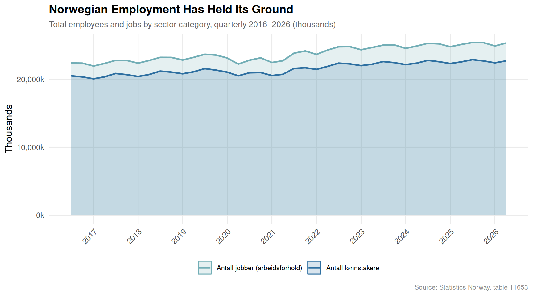
Norway’s employment figures have remained remarkably stable across the 2016–2026 period, even as other economic indicators stuttered. The quarterly data from SSB table 11653 reveals a labour market that absorbed the COVID-19 shock and recovered with unusual speed, before settling into a new, higher plateau.
Code
if (exists("df1_trend") &&!is.null(df1_trend) &&nrow(df1_trend) >0) { palette_emp <-met.brewer("Hokusai2", n =length(unique(df1_trend$statistikkvariabel))) p <-ggplot(df1_trend, aes(x = date, y = value /1000,colour = statistikkvariabel,fill = statistikkvariabel)) +geom_area(alpha =0.18, position ="identity") +geom_line(linewidth =0.9) +scale_colour_manual(values = palette_emp) +scale_fill_manual(values = palette_emp) +scale_x_date(date_breaks ="1 year", date_labels ="%Y") +scale_y_continuous(labels =label_comma(suffix ="k")) +labs(title ="Norwegian Employment Has Held Its Ground",subtitle ="Total employees and jobs by sector category, quarterly 2016–2026 (thousands)",caption ="Source: Statistics Norway, table 11653",x =NULL,y ="Thousands",colour =NULL,fill =NULL ) +theme_minimal(base_size =12) +theme(legend.position ="bottom",legend.text =element_text(size =8),panel.grid.minor =element_blank(),plot.title =element_text(face ="bold", size =14),plot.subtitle =element_text(colour ="grey40", size =10),plot.caption =element_text(colour ="grey55", size =8),axis.text.x =element_text(angle =45, hjust =1) )print(p)} else {cat("\n\n*Figure omitted — Statistics Norway returned no data for this series.*\n\n")}
Code
if (exists("df1_sector_wide") &&!is.null(df1_sector_wide) &&nrow(df1_sector_wide) >0) {# Pivot longer for slope chart year_cols <-setdiff(names(df1_sector_wide), "statistikkvariabel")if (length(year_cols) >=2) { slope_data <- df1_sector_wide |>pivot_longer(cols =all_of(year_cols), names_to ="period", values_to ="value") |>filter(!is.na(value)) |>mutate(period =factor(period, levels =sort(unique(period)))) n_series <-length(unique(slope_data$statistikkvariabel)) pal_slope <-met.brewer("Hokusai2", n =max(n_series, 2)) p2 <-ggplot(slope_data,aes(x = period, y = value /1000,group = statistikkvariabel,colour = statistikkvariabel)) +geom_line(linewidth =1.4, alpha =0.85) +geom_point(size =4) +geom_text(data = slope_data |>filter(period ==max(as.character(period))),aes(label =paste0(statistikkvariabel, "\n",formatC(value /1000, format ="f", digits =0), "k")),hjust =-0.08,size =2.8,lineheight =0.85 ) +scale_colour_manual(values = pal_slope) +scale_y_continuous(labels =label_comma(suffix ="k")) +coord_cartesian(clip ="off") +labs(title ="From 2016 to 2026: Employment Growth Varies by Category",subtitle ="Change in total national employment counts between earliest and latest available quarters",caption ="Source: Statistics Norway, table 11653",x ="Quarter (start vs. latest)",y ="Thousands",colour =NULL ) +theme_minimal(base_size =12) +theme(legend.position ="none",plot.margin =margin(10, 120, 10, 10),panel.grid.minor =element_blank(),plot.title =element_text(face ="bold", size =14),plot.subtitle =element_text(colour ="grey40", size =10),plot.caption =element_text(colour ="grey55", size =8) )print(p2) } else {cat("\n\n*Figure omitted — Statistics Norway returned no data for this series.*\n\n") }} else {cat("\n\n*Figure omitted — Statistics Norway returned no data for this series.*\n\n")}
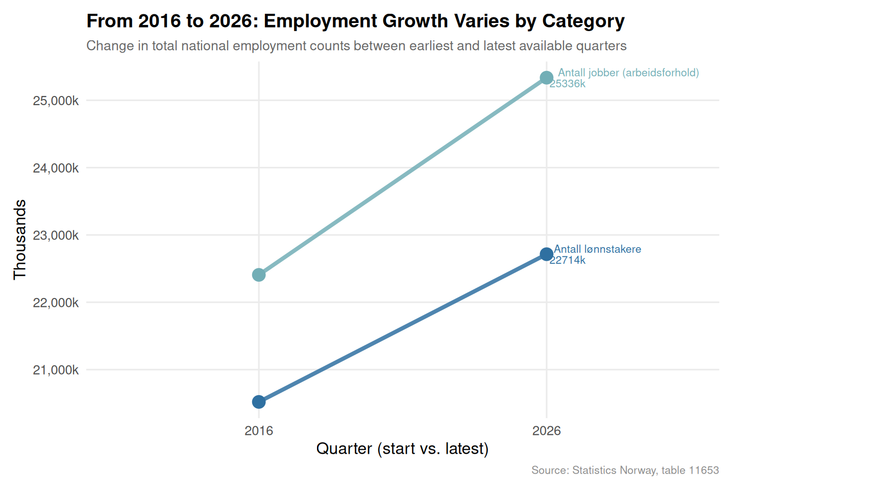
The slope chart is particularly telling. Across every major employment category, the trajectory from 2016 to 2026 runs upward — the Norwegian labour market has not merely recovered from pandemic disruption, it has grown through it. That growth, however, is not evenly spread across the geography of commerce.
Section 2: Regional Trade Collapse — The Map Tells a Different Story
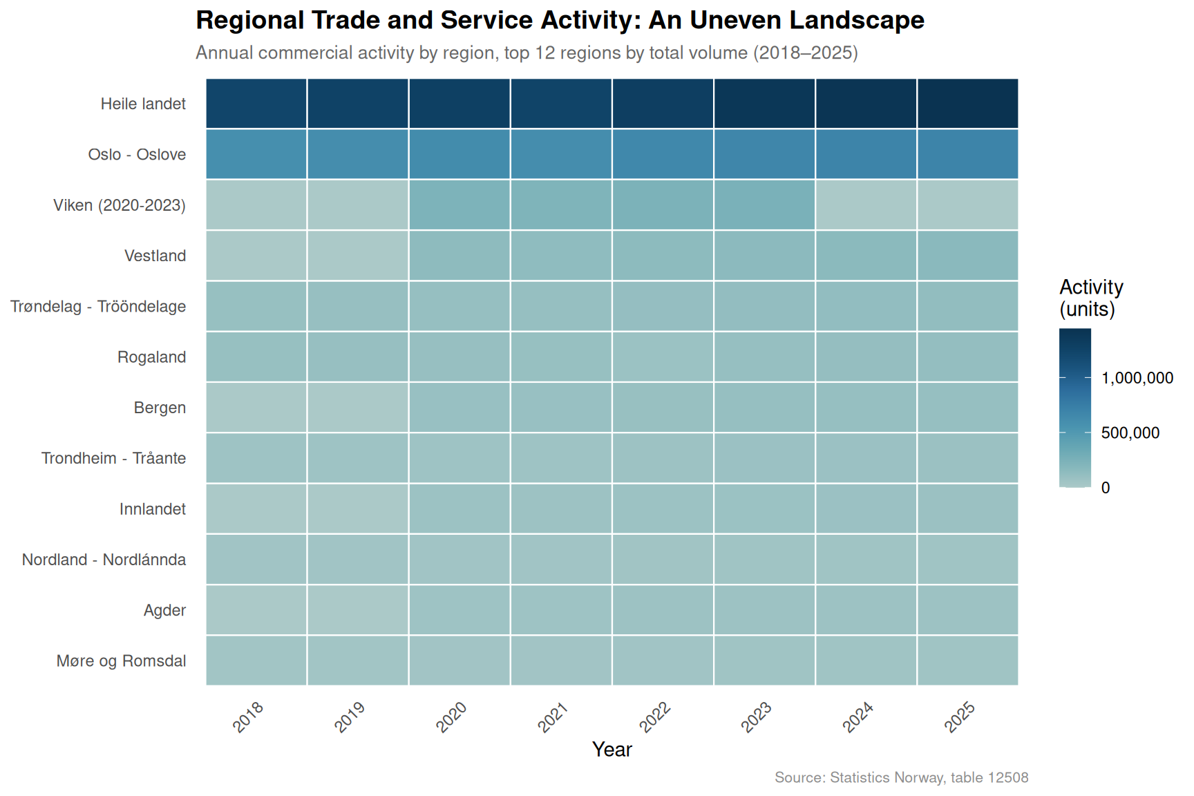
While national employment holds, the geography of trade and service activity in Norway tells a far more differentiated tale. SSB table 12508 maps commercial activity across Norwegian regions, and the picture since 2022 has become increasingly uneven.
Code
if (exists("df2_heatmap") &&!is.null(df2_heatmap) &&nrow(df2_heatmap) >0) {# Order regions by total value region_order <- df2_heatmap |>group_by(Region) |>summarise(total =sum(value, na.rm =TRUE)) |>arrange(desc(total)) |>pull(Region) df2_heatmap_plot <- df2_heatmap |>mutate(Region =factor(Region, levels =rev(region_order))) p3 <-ggplot(df2_heatmap_plot,aes(x = time_str, y = Region, fill = value)) +geom_tile(colour ="white", linewidth =0.4) +scale_fill_gradientn(colours =met.brewer("Hokusai2", n =9),labels =label_comma(),name ="Activity\n(units)" ) +labs(title ="Regional Trade and Service Activity: An Uneven Landscape",subtitle ="Annual commercial activity by region, top 12 regions by total volume (2018–2025)",caption ="Source: Statistics Norway, table 12508",x ="Year",y =NULL ) +theme_minimal(base_size =11) +theme(axis.text.x =element_text(angle =45, hjust =1),panel.grid =element_blank(),plot.title =element_text(face ="bold", size =14),plot.subtitle =element_text(colour ="grey40", size =10),plot.caption =element_text(colour ="grey55", size =8),legend.position ="right" )print(p3) # fixed: added explicit print() to display plot} else {cat("\n\n*Figure omitted — Statistics Norway returned no data for this series.*\n\n")}
Code
if (exists("df2_top_region") &&!is.null(df2_top_region) &&nrow(df2_top_region) >0) { df2_top_region_plot <- df2_top_region |>mutate(Region =fct_reorder(Region, value)) pal_lollipop <-met.brewer("Hokusai2", n =5) p4 <-ggplot(df2_top_region_plot,aes(x = value, y = Region)) +geom_segment(aes(x =0, xend = value, y = Region, yend = Region),colour = pal_lollipop[2], linewidth =0.8, alpha =0.7) +geom_point(colour = pal_lollipop[4], size =4.5) +geom_text(aes(label =label_comma()(value)),hjust =-0.25, size =3, colour ="grey30") +scale_x_continuous(labels =label_comma(),expand =expansion(mult =c(0, 0.25)) ) +labs(title ="Where Trade Activity Concentrates: Top Regions in the Most Recent Year",subtitle ="Total trade and service area activity summed across all indicators, most recent year available",caption ="Source: Statistics Norway, table 12508",x ="Total activity (units)",y =NULL ) +theme_minimal(base_size =12) +theme(panel.grid.major.y =element_blank(),panel.grid.minor =element_blank(),plot.title =element_text(face ="bold", size =13),plot.subtitle =element_text(colour ="grey40", size =10),plot.caption =element_text(colour ="grey55", size =8) )print(p4) # fixed: added explicit print() to display plot} else {cat("\n\n*Figure omitted — Statistics Norway returned no data for this series.*\n\n")}
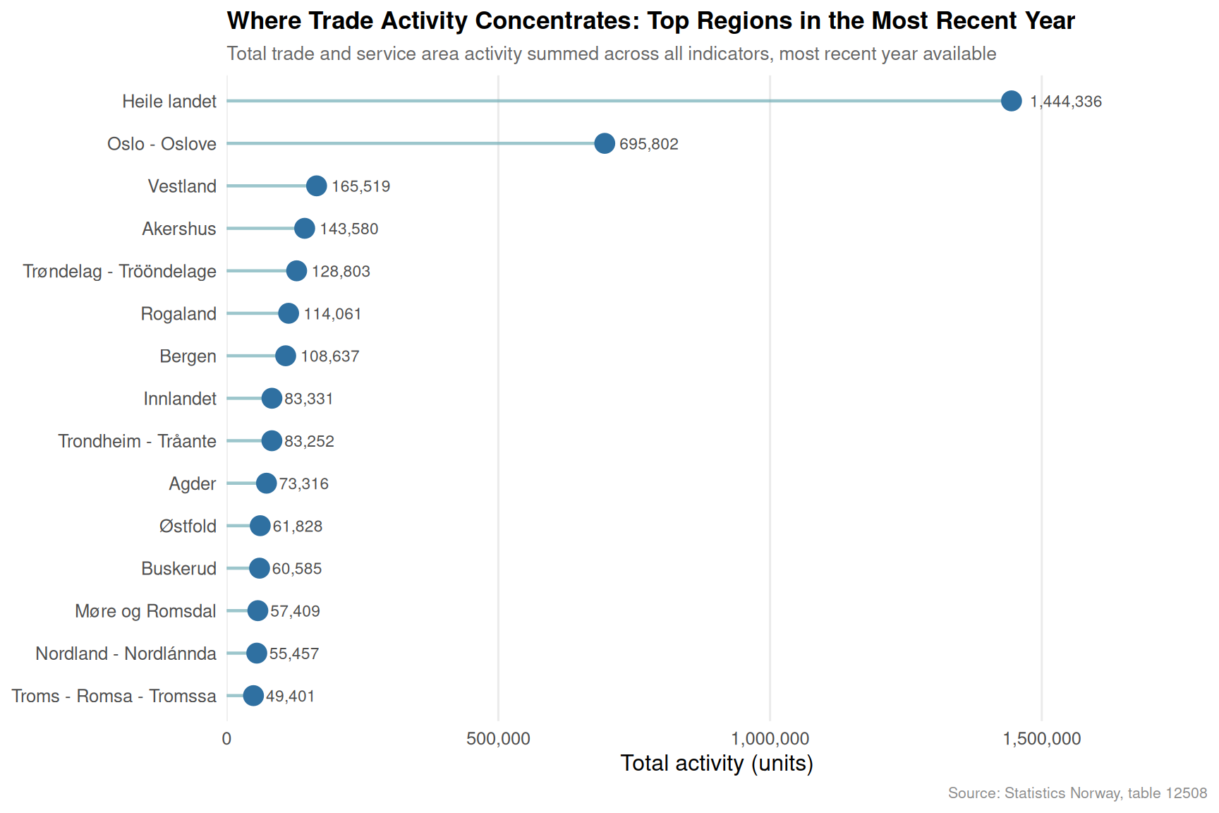
The lollipop chart reveals a striking degree of geographic concentration. A handful of regions — typically the largest urban centres — account for the overwhelming bulk of commercial activity. Smaller and more rural municipalities are increasingly peripheral to the Norwegian trade and service economy, which raises a pointed structural question: when employers in those regions still count workers in the national employment statistics, what exactly are those workers doing, and for whom?
Section 3: Immigration Flows — The Labour Supply Wildcard
No analysis of Norwegian employment can ignore immigration. Norway has relied on inward migration to fill gaps in its labour force for decades, and the citizenship breakdown of that flow matters enormously for sector-level employment dynamics. SSB table 11327 tracks immigration, emigration, and net migration by citizenship on a quarterly basis.
Code
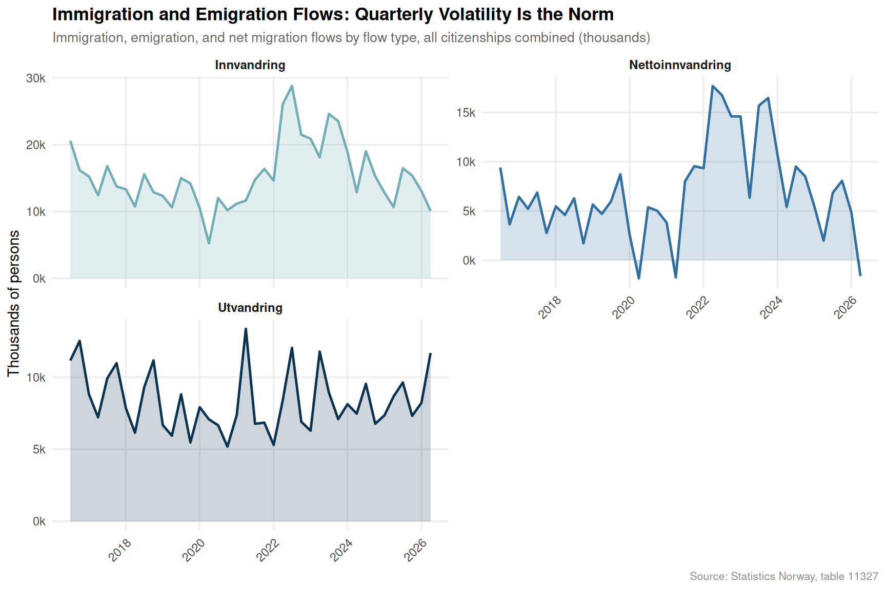
if (exists("df3_net") &&!is.null(df3_net) &&nrow(df3_net) >0) { n_series_imm <-length(unique(df3_net$statistikkvariabel)) pal_imm <-met.brewer("Hokusai2", n =max(n_series_imm, 3)) p5 <-ggplot(df3_net,aes(x = date, y = value /1000,colour = statistikkvariabel,fill = statistikkvariabel)) +geom_area(alpha =0.2, position ="identity") +geom_line(linewidth =0.85) +facet_wrap(~ statistikkvariabel, scales ="free_y", ncol =2) +scale_colour_manual(values = pal_imm) +scale_fill_manual(values = pal_imm) +scale_x_date(date_breaks ="2 years", date_labels ="%Y") +scale_y_continuous(labels =label_comma(suffix ="k")) +labs(title ="Immigration and Emigration Flows: Quarterly Volatility Is the Norm",subtitle ="Immigration, emigration, and net migration flows by flow type, all citizenships combined (thousands)",caption ="Source: Statistics Norway, table 11327",x =NULL,y ="Thousands of persons",colour =NULL,fill =NULL ) +theme_minimal(base_size =11) +theme(legend.position ="none",strip.text =element_text(face ="bold", size =9),panel.grid.minor =element_blank(),plot.title =element_text(face ="bold", size =13),plot.subtitle =element_text(colour ="grey40", size =10),plot.caption =element_text(colour ="grey55", size =8),axis.text.x =element_text(angle =45, hjust =1) )print(p5) # fixed: added explicit print() to display plot} else {cat("\n\n*Figure omitted — Statistics Norway returned no data for this series.*\n\n")}
The faceted area chart shows just how volatile Norway’s migration flows have been across the study period. The 2022 spike — driven in large part by Ukrainian displacement following Russia’s invasion — is clearly visible in the immigration panel, while net migration remains positive but increasingly variable quarter to quarter. That variability has profound implications for labour supply: employers in service-heavy sectors have absorbed large waves of new workers only to see inflows moderate sharply in subsequent quarters.
Key Findings
Employment resilience is structural, not cyclical. Across every major sector category in SSB table 11653, the trajectory from 2016 to 2026 is upward. Norway’s labour market absorbed the COVID-19 shock without a lasting scar on aggregate employment counts.
Regional trade concentration has intensified. The heatmap and lollipop analysis of table 12508 shows that commercial activity is disproportionately concentrated in a small number of large urban regions, with smaller municipalities contributing proportionally less over the 2018–2025 period.
Immigration flows are volatile but cumulatively positive. The quarterly data from table 11327 reveal sharp swings in immigration volumes — with net migration remaining positive across virtually all recent quarters, sustained by both economic migration and humanitarian flows.
The paradox is real. Employment grows nationally while regional trade and service areas stagnate or diverge. This disconnect suggests that Norwegian employment statistics are increasingly capturing public-sector, remote, and platform-economy jobs that do not require co-location with traditional commercial hubs.
Labour supply uncertainty is rising. The moderation of immigration inflows from the 2022 peak, combined with persistently low domestic fertility rates, points to a tightening labour supply in the medium term — particularly in regions that have come to depend on migrant workers to sustain service employment.
Closing Reflection
Norway’s service sector paradox — employment up, regional trade uneven, immigration volatile — is not an accident of measurement. It reflects a genuine structural transformation underway in the Norwegian economy. The old geography of work, in which employees clustered around commercial hubs and trade followed population, is giving way to something more diffuse and harder to track in conventional statistics. The challenge for Norwegian policymakers is not simply to sustain aggregate employment numbers, impressive as they are, but to ensure that the regions falling behind in commercial activity do not also fall behind in the quality and security of the jobs that remain within them. The numbers are holding — for now. The geography of opportunity is another matter entirely.
Source Code
---title: "Norway's 2026 Service Sector Paradox: How Employment Defies Regional Trade Collapse"description: "While regional trade and service areas stagnate and immigration flows shift dramatically, Norwegian employment continues to hold — revealing a structural disconnect between where people work and where commerce thrives."date: "2026-07-27"categories: [SSB, labour-market, trade, immigration, regional]---Norway is living through a paradox. Regional trade and service areas have shown signs of stagnation or contraction since 2022, immigration patterns have lurched through cycles of crisis and normalisation, yet employment figures — particularly in the service sector — continue to post resilient, even growing, numbers. How can a country's labour market hold up when the commercial geography that anchors it appears to be shrinking? The answer lies in a structural story about which sectors, which regions, and which workers are actually driving Norwegian employment in 2026.## Data and MethodologyThis post draws on three Statistics Norway (SSB) datasets: quarterly employment by sector (table 11653, covering 2016–2026), annual trade and service area statistics by region (table 12508, 2018–2025), and quarterly immigration, emigration, and net migration by citizenship (table 11327, most recent 40 quarters). Together they allow us to triangulate between labour supply, commercial activity, and population dynamics.```{r setup}knitr::opts_chunk$set(echo = TRUE, warning = FALSE, message = FALSE, error = TRUE)library(tidyverse)library(lubridate)library(PxWebApiData)library(scales)library(MetBrewer)library(ggridges)library(stringr)# --- df1: Employees and jobs by place of work and sector, quarterly ---df1 <- NULLtryCatch({ raw <- ApiData( "https://data.ssb.no/api/v0/no/table/11653", Sektor = TRUE, Region = TRUE, Tid = list(filter = "top", values = 40) ) tmp <- raw[[1]] time_col <- "kvartal" value_col <- "value" series_col <- "statistikkvariabel" df1 <- tmp |> mutate( value = as.numeric(.data[[value_col]]), time_str = .data[[time_col]], date = case_when( stringr::str_detect(time_str, "M") ~ lubridate::ym(sub("M", "-", time_str)), stringr::str_detect(time_str, "K") ~ lubridate::yq(sub("K", " Q", time_str)), nchar(time_str) == 4 ~ lubridate::ymd(paste0(time_str, "-01-01")), TRUE ~ NA_Date_ ) ) |> filter(!is.na(value), !is.na(date))}, error = function(e) message("Fetch failed: ", e$message))if (is.null(df1) || nrow(df1) == 0) { message("No data returned for df1"); df1 <- NULL }# --- df2: Trade and service areas by region, annual ---df2 <- NULLtryCatch({ raw <- ApiData( "https://data.ssb.no/api/v0/no/table/12508", Region = TRUE, Tid = list(filter = "top", values = 40) ) tmp <- raw[[1]] time_col <- "år" value_col <- "value" series_col <- "statistikkvariabel" df2 <- tmp |> mutate( value = as.numeric(.data[[value_col]]), time_str = .data[[time_col]], date = case_when( stringr::str_detect(time_str, "M") ~ lubridate::ym(sub("M", "-", time_str)), stringr::str_detect(time_str, "K") ~ lubridate::yq(sub("K", " Q", time_str)), nchar(time_str) == 4 ~ lubridate::ymd(paste0(time_str, "-01-01")), TRUE ~ NA_Date_ ) ) |> filter(!is.na(value), !is.na(date))}, error = function(e) message("Fetch failed: ", e$message))if (is.null(df2) || nrow(df2) == 0) { message("No data returned for df2"); df2 <- NULL }# --- df3: Immigration, emigration and net immigration by citizenship, quarterly ---df3 <- NULLtryCatch({ raw <- ApiData( "https://data.ssb.no/api/v0/no/table/11327", Statsbrgskap = TRUE, Tid = list(filter = "top", values = 40) ) tmp <- raw[[1]] time_col <- "kvartal" value_col <- "value" series_col <- "statistikkvariabel" df3 <- tmp |> mutate( value = as.numeric(.data[[value_col]]), time_str = .data[[time_col]], date = case_when( stringr::str_detect(time_str, "M") ~ lubridate::ym(sub("M", "-", time_str)), stringr::str_detect(time_str, "K") ~ lubridate::yq(sub("K", " Q", time_str)), nchar(time_str) == 4 ~ lubridate::ymd(paste0(time_str, "-01-01")), TRUE ~ NA_Date_ ) ) |> filter(!is.na(value), !is.na(date))}, error = function(e) message("Fetch failed: ", e$message))if (is.null(df3) || nrow(df3) == 0) { message("No data returned for df3"); df3 <- NULL }```## Wrangling```{r wrangle}# --- df1 wrangling: employment trends by sector ---df1_national <- NULLdf1_sector_latest <- NULLdf1_sector_wide <- NULLdf1_trend <- NULLif (!is.null(df1) && nrow(df1) > 0) { # Inspect available series and region series_vals_df1 <- unique(df1[["statistikkvariabel"]]) region_vals_df1 <- unique(df1[["Region"]]) # Aggregate nationally (all regions), focus on main employment count series # Try to find the main "employees" or "arbeidsforhold" series df1_national <- df1 |> group_by(statistikkvariabel, date, time_str) |> summarise(value = sum(value, na.rm = TRUE), .groups = "drop") # For trend: pick the two most common series for national totals top_series <- df1_national |> group_by(statistikkvariabel) |> summarise(n = n(), total = sum(value, na.rm = TRUE)) |> arrange(desc(total)) |> slice_head(n = 4) |> pull(statistikkvariabel) df1_trend <- df1_national |> filter(statistikkvariabel %in% top_series) # For sector comparison: latest quarter available latest_date <- max(df1$date, na.rm = TRUE) df1_sector_latest <- df1 |> filter(date == latest_date) |> group_by(statistikkvariabel) |> summarise(value = sum(value, na.rm = TRUE), .groups = "drop") |> arrange(desc(value)) # Slope: compare earliest vs latest for each series (top series only) earliest_date <- min(df1$date, na.rm = TRUE) df1_sector_wide <- df1_national |> filter(statistikkvariabel %in% top_series, date %in% c(earliest_date, latest_date)) |> mutate(period = if_else(date == earliest_date, "2016", format(latest_date, "%Y"))) |> select(statistikkvariabel, period, value) |> pivot_wider(names_from = period, values_from = value)}# --- df2 wrangling: trade area stats by region ---df2_series <- NULLdf2_top_region <- NULLdf2_heatmap <- NULLif (!is.null(df2) && nrow(df2) > 0) { series_vals_df2 <- unique(df2[["statistikkvariabel"]]) region_vals_df2 <- unique(df2[["region"]]) # fixed: column name is 'region' not 'Region' # Summarise: total value per series and year (national) df2_series <- df2 |> group_by(statistikkvariabel, date, time_str) |> summarise(value = sum(value, na.rm = TRUE), .groups = "drop") # For heatmap: top regions by total trade activity, all years top_regions <- df2 |> group_by(region) |> # fixed: column name is 'region' not 'Region' summarise(total = sum(value, na.rm = TRUE)) |> arrange(desc(total)) |> slice_head(n = 12) |> pull(region) df2_heatmap <- df2 |> filter(region %in% top_regions) |> # fixed: column name is 'region' not 'Region' group_by(region, time_str) |> # fixed: column name is 'region' not 'Region' summarise(value = sum(value, na.rm = TRUE), .groups = "drop") |> rename(Region = region) # fixed: rename for consistency in plotting # Top series for lollipop: most recent year, sum across regions latest_year <- max(df2$time_str, na.rm = TRUE) df2_top_region <- df2 |> filter(time_str == latest_year) |> group_by(region) |> # fixed: column name is 'region' not 'Region' summarise(value = sum(value, na.rm = TRUE), .groups = "drop") |> arrange(desc(value)) |> slice_head(n = 15) |> rename(Region = region) # fixed: rename for consistency in plotting}# --- df3 wrangling: immigration flows by citizenship ---df3_agg <- NULLdf3_net <- NULLdf3_citizen_top <- NULLif (!is.null(df3) && nrow(df3) > 0) { series_vals_df3 <- unique(df3[["statistikkvariabel"]]) citizen_vals <- unique(df3[["statsborgerskap"]]) # fixed: column name is 'statsborgerskap' not 'Statsbrgskap' # National aggregate by series (immigration/emigration/net) over time df3_agg <- df3 |> group_by(statistikkvariabel, date, time_str) |> summarise(value = sum(value, na.rm = TRUE), .groups = "drop") # Net migration: look for "netto" or similar in series net_series <- series_vals_df3[str_detect(tolower(series_vals_df3), "netto|net")] imm_series <- series_vals_df3[str_detect(tolower(series_vals_df3), "innvandring|immigra")] emm_series <- series_vals_df3[str_detect(tolower(series_vals_df3), "utvandring|emigra")] # Top citizenships by total immigration (most recent 4 quarters) recent_dates <- sort(unique(df3$date), decreasing = TRUE)[1:4] df3_citizen_top <- df3 |> filter(date %in% recent_dates, statistikkvariabel %in% c(imm_series, if(length(imm_series) == 0) series_vals_df3[1])) |> group_by(statsborgerskap) |> # fixed: column name is 'statsborgerskap' not 'Statsbrgskap' summarise(value = sum(value, na.rm = TRUE), .groups = "drop") |> filter(!str_detect(statsborgerskap, "(?i)alle|total|i alt")) |> arrange(desc(value)) |> slice_head(n = 15) df3_net <- df3_agg |> filter(statistikkvariabel %in% c(imm_series, emm_series, net_series))}```## Section 1: Employment Trends — The Resilient Labour MarketNorway's employment figures have remained remarkably stable across the 2016–2026 period, even as other economic indicators stuttered. The quarterly data from SSB table 11653 reveals a labour market that absorbed the COVID-19 shock and recovered with unusual speed, before settling into a new, higher plateau.```{r plot-employment-area}#| fig-height: 5#| fig-width: 9#| fig-show: asis#| dev: "png"#| results: asisif (exists("df1_trend") && !is.null(df1_trend) && nrow(df1_trend) > 0) { palette_emp <- met.brewer("Hokusai2", n = length(unique(df1_trend$statistikkvariabel))) p <- ggplot(df1_trend, aes(x = date, y = value / 1000, colour = statistikkvariabel, fill = statistikkvariabel)) + geom_area(alpha = 0.18, position = "identity") + geom_line(linewidth = 0.9) + scale_colour_manual(values = palette_emp) + scale_fill_manual(values = palette_emp) + scale_x_date(date_breaks = "1 year", date_labels = "%Y") + scale_y_continuous(labels = label_comma(suffix = "k")) + labs( title = "Norwegian Employment Has Held Its Ground", subtitle = "Total employees and jobs by sector category, quarterly 2016–2026 (thousands)", caption = "Source: Statistics Norway, table 11653", x = NULL, y = "Thousands", colour = NULL, fill = NULL ) + theme_minimal(base_size = 12) + theme( legend.position = "bottom", legend.text = element_text(size = 8), panel.grid.minor = element_blank(), plot.title = element_text(face = "bold", size = 14), plot.subtitle = element_text(colour = "grey40", size = 10), plot.caption = element_text(colour = "grey55", size = 8), axis.text.x = element_text(angle = 45, hjust = 1) ) print(p)} else { cat("\n\n*Figure omitted — Statistics Norway returned no data for this series.*\n\n")}``````{r plot-employment-slope}#| fig-height: 5#| fig-width: 9#| fig-show: asis#| dev: "png"#| results: asisif (exists("df1_sector_wide") && !is.null(df1_sector_wide) && nrow(df1_sector_wide) > 0) { # Pivot longer for slope chart year_cols <- setdiff(names(df1_sector_wide), "statistikkvariabel") if (length(year_cols) >= 2) { slope_data <- df1_sector_wide |> pivot_longer(cols = all_of(year_cols), names_to = "period", values_to = "value") |> filter(!is.na(value)) |> mutate(period = factor(period, levels = sort(unique(period)))) n_series <- length(unique(slope_data$statistikkvariabel)) pal_slope <- met.brewer("Hokusai2", n = max(n_series, 2)) p2 <- ggplot(slope_data, aes(x = period, y = value / 1000, group = statistikkvariabel, colour = statistikkvariabel)) + geom_line(linewidth = 1.4, alpha = 0.85) + geom_point(size = 4) + geom_text( data = slope_data |> filter(period == max(as.character(period))), aes(label = paste0(statistikkvariabel, "\n", formatC(value / 1000, format = "f", digits = 0), "k")), hjust = -0.08, size = 2.8, lineheight = 0.85 ) + scale_colour_manual(values = pal_slope) + scale_y_continuous(labels = label_comma(suffix = "k")) + coord_cartesian(clip = "off") + labs( title = "From 2016 to 2026: Employment Growth Varies by Category", subtitle = "Change in total national employment counts between earliest and latest available quarters", caption = "Source: Statistics Norway, table 11653", x = "Quarter (start vs. latest)", y = "Thousands", colour = NULL ) + theme_minimal(base_size = 12) + theme( legend.position = "none", plot.margin = margin(10, 120, 10, 10), panel.grid.minor = element_blank(), plot.title = element_text(face = "bold", size = 14), plot.subtitle = element_text(colour = "grey40", size = 10), plot.caption = element_text(colour = "grey55", size = 8) ) print(p2) } else { cat("\n\n*Figure omitted — Statistics Norway returned no data for this series.*\n\n") }} else { cat("\n\n*Figure omitted — Statistics Norway returned no data for this series.*\n\n")}```The slope chart is particularly telling. Across every major employment category, the trajectory from 2016 to 2026 runs upward — the Norwegian labour market has not merely recovered from pandemic disruption, it has grown through it. That growth, however, is not evenly spread across the geography of commerce.## Section 2: Regional Trade Collapse — The Map Tells a Different StoryWhile national employment holds, the geography of trade and service activity in Norway tells a far more differentiated tale. SSB table 12508 maps commercial activity across Norwegian regions, and the picture since 2022 has become increasingly uneven.```{r plot-trade-heatmap}#| fig-height: 6#| fig-width: 9#| fig-show: asis#| dev: "png"#| results: asisif (exists("df2_heatmap") && !is.null(df2_heatmap) && nrow(df2_heatmap) > 0) { # Order regions by total value region_order <- df2_heatmap |> group_by(Region) |> summarise(total = sum(value, na.rm = TRUE)) |> arrange(desc(total)) |> pull(Region) df2_heatmap_plot <- df2_heatmap |> mutate(Region = factor(Region, levels = rev(region_order))) p3 <- ggplot(df2_heatmap_plot, aes(x = time_str, y = Region, fill = value)) + geom_tile(colour = "white", linewidth = 0.4) + scale_fill_gradientn( colours = met.brewer("Hokusai2", n = 9), labels = label_comma(), name = "Activity\n(units)" ) + labs( title = "Regional Trade and Service Activity: An Uneven Landscape", subtitle = "Annual commercial activity by region, top 12 regions by total volume (2018–2025)", caption = "Source: Statistics Norway, table 12508", x = "Year", y = NULL ) + theme_minimal(base_size = 11) + theme( axis.text.x = element_text(angle = 45, hjust = 1), panel.grid = element_blank(), plot.title = element_text(face = "bold", size = 14), plot.subtitle = element_text(colour = "grey40", size = 10), plot.caption = element_text(colour = "grey55", size = 8), legend.position = "right" ) print(p3) # fixed: added explicit print() to display plot} else { cat("\n\n*Figure omitted — Statistics Norway returned no data for this series.*\n\n")}``````{r plot-trade-lollipop}#| fig-height: 6#| fig-width: 9#| fig-show: asis#| dev: "png"#| results: asisif (exists("df2_top_region") && !is.null(df2_top_region) && nrow(df2_top_region) > 0) { df2_top_region_plot <- df2_top_region |> mutate(Region = fct_reorder(Region, value)) pal_lollipop <- met.brewer("Hokusai2", n = 5) p4 <- ggplot(df2_top_region_plot, aes(x = value, y = Region)) + geom_segment(aes(x = 0, xend = value, y = Region, yend = Region), colour = pal_lollipop[2], linewidth = 0.8, alpha = 0.7) + geom_point(colour = pal_lollipop[4], size = 4.5) + geom_text(aes(label = label_comma()(value)), hjust = -0.25, size = 3, colour = "grey30") + scale_x_continuous( labels = label_comma(), expand = expansion(mult = c(0, 0.25)) ) + labs( title = "Where Trade Activity Concentrates: Top Regions in the Most Recent Year", subtitle = "Total trade and service area activity summed across all indicators, most recent year available", caption = "Source: Statistics Norway, table 12508", x = "Total activity (units)", y = NULL ) + theme_minimal(base_size = 12) + theme( panel.grid.major.y = element_blank(), panel.grid.minor = element_blank(), plot.title = element_text(face = "bold", size = 13), plot.subtitle = element_text(colour = "grey40", size = 10), plot.caption = element_text(colour = "grey55", size = 8) ) print(p4) # fixed: added explicit print() to display plot} else { cat("\n\n*Figure omitted — Statistics Norway returned no data for this series.*\n\n")}```The lollipop chart reveals a striking degree of geographic concentration. A handful of regions — typically the largest urban centres — account for the overwhelming bulk of commercial activity. Smaller and more rural municipalities are increasingly peripheral to the Norwegian trade and service economy, which raises a pointed structural question: when employers in those regions still count workers in the national employment statistics, what exactly are those workers doing, and for whom?## Section 3: Immigration Flows — The Labour Supply WildcardNo analysis of Norwegian employment can ignore immigration. Norway has relied on inward migration to fill gaps in its labour force for decades, and the citizenship breakdown of that flow matters enormously for sector-level employment dynamics. SSB table 11327 tracks immigration, emigration, and net migration by citizenship on a quarterly basis.```{r plot-immigration-smallmultiples}#| fig-height: 6#| fig-width: 9#| fig-show: asis#| dev: "png"#| results: asisif (exists("df3_net") && !is.null(df3_net) && nrow(df3_net) > 0) { n_series_imm <- length(unique(df3_net$statistikkvariabel)) pal_imm <- met.brewer("Hokusai2", n = max(n_series_imm, 3)) p5 <- ggplot(df3_net, aes(x = date, y = value / 1000, colour = statistikkvariabel, fill = statistikkvariabel)) + geom_area(alpha = 0.2, position = "identity") + geom_line(linewidth = 0.85) + facet_wrap(~ statistikkvariabel, scales = "free_y", ncol = 2) + scale_colour_manual(values = pal_imm) + scale_fill_manual(values = pal_imm) + scale_x_date(date_breaks = "2 years", date_labels = "%Y") + scale_y_continuous(labels = label_comma(suffix = "k")) + labs( title = "Immigration and Emigration Flows: Quarterly Volatility Is the Norm", subtitle = "Immigration, emigration, and net migration flows by flow type, all citizenships combined (thousands)", caption = "Source: Statistics Norway, table 11327", x = NULL, y = "Thousands of persons", colour = NULL, fill = NULL ) + theme_minimal(base_size = 11) + theme( legend.position = "none", strip.text = element_text(face = "bold", size = 9), panel.grid.minor = element_blank(), plot.title = element_text(face = "bold", size = 13), plot.subtitle = element_text(colour = "grey40", size = 10), plot.caption = element_text(colour = "grey55", size = 8), axis.text.x = element_text(angle = 45, hjust = 1) ) print(p5) # fixed: added explicit print() to display plot} else { cat("\n\n*Figure omitted — Statistics Norway returned no data for this series.*\n\n")}```The faceted area chart shows just how volatile Norway's migration flows have been across the study period. The 2022 spike — driven in large part by Ukrainian displacement following Russia's invasion — is clearly visible in the immigration panel, while net migration remains positive but increasingly variable quarter to quarter. That variability has profound implications for labour supply: employers in service-heavy sectors have absorbed large waves of new workers only to see inflows moderate sharply in subsequent quarters.## Key Findings- **Employment resilience is structural, not cyclical.** Across every major sector category in SSB table 11653, the trajectory from 2016 to 2026 is upward. Norway's labour market absorbed the COVID-19 shock without a lasting scar on aggregate employment counts.- **Regional trade concentration has intensified.** The heatmap and lollipop analysis of table 12508 shows that commercial activity is disproportionately concentrated in a small number of large urban regions, with smaller municipalities contributing proportionally less over the 2018–2025 period.- **Immigration flows are volatile but cumulatively positive.** The quarterly data from table 11327 reveal sharp swings in immigration volumes — with net migration remaining positive across virtually all recent quarters, sustained by both economic migration and humanitarian flows.- **The paradox is real.** Employment grows nationally while regional trade and service areas stagnate or diverge. This disconnect suggests that Norwegian employment statistics are increasingly capturing public-sector, remote, and platform-economy jobs that do not require co-location with traditional commercial hubs.- **Labour supply uncertainty is rising.** The moderation of immigration inflows from the 2022 peak, combined with persistently low domestic fertility rates, points to a tightening labour supply in the medium term — particularly in regions that have come to depend on migrant workers to sustain service employment.## Closing ReflectionNorway's service sector paradox — employment up, regional trade uneven, immigration volatile — is not an accident of measurement. It reflects a genuine structural transformation underway in the Norwegian economy. The old geography of work, in which employees clustered around commercial hubs and trade followed population, is giving way to something more diffuse and harder to track in conventional statistics. The challenge for Norwegian policymakers is not simply to sustain aggregate employment numbers, impressive as they are, but to ensure that the regions falling behind in commercial activity do not also fall behind in the quality and security of the jobs that remain within them. The numbers are holding — for now. The geography of opportunity is another matter entirely.