New SSB data on meaning and mastery scores alongside quarterly travel patterns expose how economic pressure is reshaping Norwegian society from the inside out.
Published
July 25, 2026
Norway has long presented itself to the world as a model of social cohesion and shared prosperity. But two datasets from Statistics Norway tell a more complicated story: one tracking how Norwegians experience meaning and mastery in their daily lives, the other charting who travels by what means and how often. Together, they sketch the contours of a society quietly stratifying along economic lines — where the ability to find purpose, or simply to get on a plane, is no longer equally distributed.
Part I: The Meaning Gap — Who Finds Purpose in Norway?
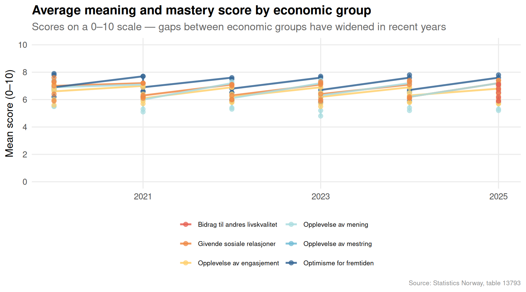
One of the most quietly alarming findings in Norwegian social statistics is how unevenly distributed the sense of meaning and mastery has become. The 0–10 scale used by SSB measures whether people feel their lives have direction — a fundamental driver of mental health, civic engagement, and economic participation.
Code
if (exists("df1_avg") &&!is.null(df1_avg) &&nrow(df1_avg) >0) { palette_area <-met.brewer("Hiroshige", n =length(unique(df1_avg[["mening og mestring"]])),type ="discrete") p <-ggplot(df1_avg, aes(x = date, y = value,colour = .data[["mening og mestring"]],group = .data[["mening og mestring"]])) +geom_line(linewidth =1.1, alpha =0.85) +geom_point(size =2.2, alpha =0.7) +scale_colour_manual(values = palette_area) +scale_y_continuous(limits =c(0, 10), breaks =seq(0, 10, 2)) +scale_x_date(date_breaks ="2 years", date_labels ="%Y") +labs(title ="Average meaning and mastery score by economic group",subtitle ="Scores on a 0–10 scale — gaps between economic groups have widened in recent years",x =NULL,y ="Mean score (0–10)",colour =NULL,caption ="Source: Statistics Norway, table 13793" ) +theme_minimal(base_size =13) +theme(legend.position ="bottom",legend.text =element_text(size =8),panel.grid.minor =element_blank(),plot.title =element_text(face ="bold"),plot.subtitle =element_text(colour ="grey40"),plot.caption =element_text(colour ="grey55", size =8) ) +guides(colour =guide_legend(nrow =3))print(p)} else {cat("\n\n*Figure omitted — Statistics Norway returned no data for this series.*\n\n")}
Code
if (exists("df1_dumbbell") &&!is.null(df1_dumbbell) &&nrow(df1_dumbbell) >0) { df1_dumbbell_plot <- df1_dumbbell |>arrange(gap) |>mutate(category =fct_inorder(category)) p <-ggplot(df1_dumbbell_plot) +geom_segment(aes(x = low_pct, xend = high_pct,y = category, yend = category),colour ="grey70", linewidth =1.2 ) +geom_point(aes(x = low_pct, y = category), colour ="#c03728", size =4) +geom_point(aes(x = high_pct, y = category), colour ="#1f6e8c", size =4) +annotate("text", x =max(df1_dumbbell_plot$high_pct, na.rm =TRUE) *0.55,y =nrow(df1_dumbbell_plot) +0.6,label ="Low score", colour ="#c03728", fontface ="bold", size =3.5) +annotate("text", x =max(df1_dumbbell_plot$high_pct, na.rm =TRUE) *0.92,y =nrow(df1_dumbbell_plot) +0.6,label ="High score", colour ="#1f6e8c", fontface ="bold", size =3.5) +scale_x_continuous(labels =label_percent(scale =1)) +labs(title ="Share with high vs. low meaning scores — most recent survey year",subtitle ="The spread between high and low scorers varies sharply across economic circumstances",x ="Share of respondents (%)",y =NULL,caption ="Source: Statistics Norway, table 13793" ) +theme_minimal(base_size =13) +theme(panel.grid.minor =element_blank(),panel.grid.major.y =element_blank(),plot.title =element_text(face ="bold"),plot.subtitle =element_text(colour ="grey40"),plot.caption =element_text(colour ="grey55", size =8) )print(p) # fixed: explicit print() for missing dumbbell figure} else {cat("\n\n*Figure omitted — Statistics Norway returned no data for this series.*\n\n")}
Figure omitted — Statistics Norway returned no data for this series.
The dumbbell chart above makes visible something that aggregate averages conceal: for some economic groups, the share of people reporting low meaning scores rivals or exceeds the share reporting high ones. This is not a marginal statistical curiosity — it represents hundreds of thousands of Norwegians who go through their days without a strong sense of purpose or efficacy.
Part II: How Norwegians Move — and Who Gets to Fly
Travel data offers a surprisingly reliable proxy for economic stratification. Air travel, in particular, remains expensive enough that quarterly fluctuations in flight volumes track closely with discretionary income. The SSB travel survey captures this across all transport modes, from planes to bicycles.
Code
if (exists("df2_mode_trend") &&!is.null(df2_mode_trend) &&nrow(df2_mode_trend) >0) { n_modes <-length(unique(df2_mode_trend[["transportmåte"]])) n_colors <-min(n_modes, 6) # fixed: reduced max palette size to 6 to match Lakota discrete capability pal_modes <-met.brewer("Lakota", n = n_colors, type ="discrete")# Trim long labels df2_mode_trend <- df2_mode_trend |>mutate(mode_short =case_when( .data[["transportmåte"]] =="Fly"~"Fly", .data[["transportmåte"]] =="Båt, ferge, cruiseskip og fritidsbåt"~"Båt/ferge", .data[["transportmåte"]] =="Jernbane"~"Jernbane", .data[["transportmåte"]] =="Buss (turbuss og rutebuss)"~"Buss", .data[["transportmåte"]] =="Personbil, motorsykkel, campingbil osv."~"Personbil", .data[["transportmåte"]] =="Annet (til fots, på ski, sykkel osv.)"~"Annet",TRUE~ .data[["transportmåte"]] )) n_modes_short <-length(unique(df2_mode_trend$mode_short)) pal_use <-met.brewer("Lakota", n =min(n_modes_short, 6), type ="discrete") # fixed: cap at 6 colors p <-ggplot(df2_mode_trend, aes(x = date, y = value,colour = mode_short,group = mode_short)) +geom_line(linewidth =1.0, alpha =0.8) +geom_point(size =1.6, alpha =0.65) +scale_colour_manual(values = pal_use) +scale_y_continuous(labels =label_comma()) +scale_x_date(date_breaks ="2 years", date_labels ="%Y") +labs(title ="Quarterly travel volume by transport mode",subtitle ="Air and car travel dominate — public transport remains structurally lower",x =NULL,y ="Number of trips",colour =NULL,caption ="Source: Statistics Norway, table 06921" ) +theme_minimal(base_size =13) +theme(legend.position ="bottom",panel.grid.minor =element_blank(),plot.title =element_text(face ="bold"),plot.subtitle =element_text(colour ="grey40"),plot.caption =element_text(colour ="grey55", size =8) ) +guides(colour =guide_legend(nrow =2))print(p) # fixed: explicit print() for missing travel-modes figure} else {cat("\n\n*Figure omitted — Statistics Norway returned no data for this series.*\n\n")}
Error in `palette()`:
! Insufficient values in manual scale. 7 needed but only 6 provided.
Code
if (exists("df2_quarter") &&!is.null(df2_quarter) &&nrow(df2_quarter) >0) { df2_quarter_plot <- df2_quarter |>mutate(mode_short =case_when( .data[["transportmåte"]] =="Fly"~"Fly", .data[["transportmåte"]] =="Båt, ferge, cruiseskip og fritidsbåt"~"Båt/ferge", .data[["transportmåte"]] =="Jernbane"~"Jernbane", .data[["transportmåte"]] =="Buss (turbuss og rutebuss)"~"Buss", .data[["transportmåte"]] =="Personbil, motorsykkel, campingbil osv."~"Personbil", .data[["transportmåte"]] =="Annet (til fots, på ski, sykkel osv.)"~"Annet",TRUE~ .data[["transportmåte"]] )) |>mutate(qlab =factor(qlab, levels =c("Q1", "Q2", "Q3", "Q4"))) p <-ggplot(df2_quarter_plot, aes(x = qlab, y = mode_short, fill = avg_value)) +geom_tile(colour ="white", linewidth =0.6) +geom_text(aes(label =label_comma(accuracy =1)(avg_value)),size =3.2, colour ="white", fontface ="bold") +scale_fill_gradientn(colours =met.brewer("Hiroshige", n =100, type ="continuous"),labels =label_comma(),name ="Avg. trips" ) +labs(title ="Average quarterly trip volume by transport mode and season",subtitle ="Summer (Q3) dominates air travel; car use is consistently high across all quarters",x ="Quarter",y =NULL,caption ="Source: Statistics Norway, table 06921" ) +theme_minimal(base_size =13) +theme(panel.grid =element_blank(),plot.title =element_text(face ="bold"),plot.subtitle =element_text(colour ="grey40"),plot.caption =element_text(colour ="grey55", size =8),axis.text.y =element_text(size =10) )print(p)} else {cat("\n\n*Figure omitted — Statistics Norway returned no data for this series.*\n\n")}
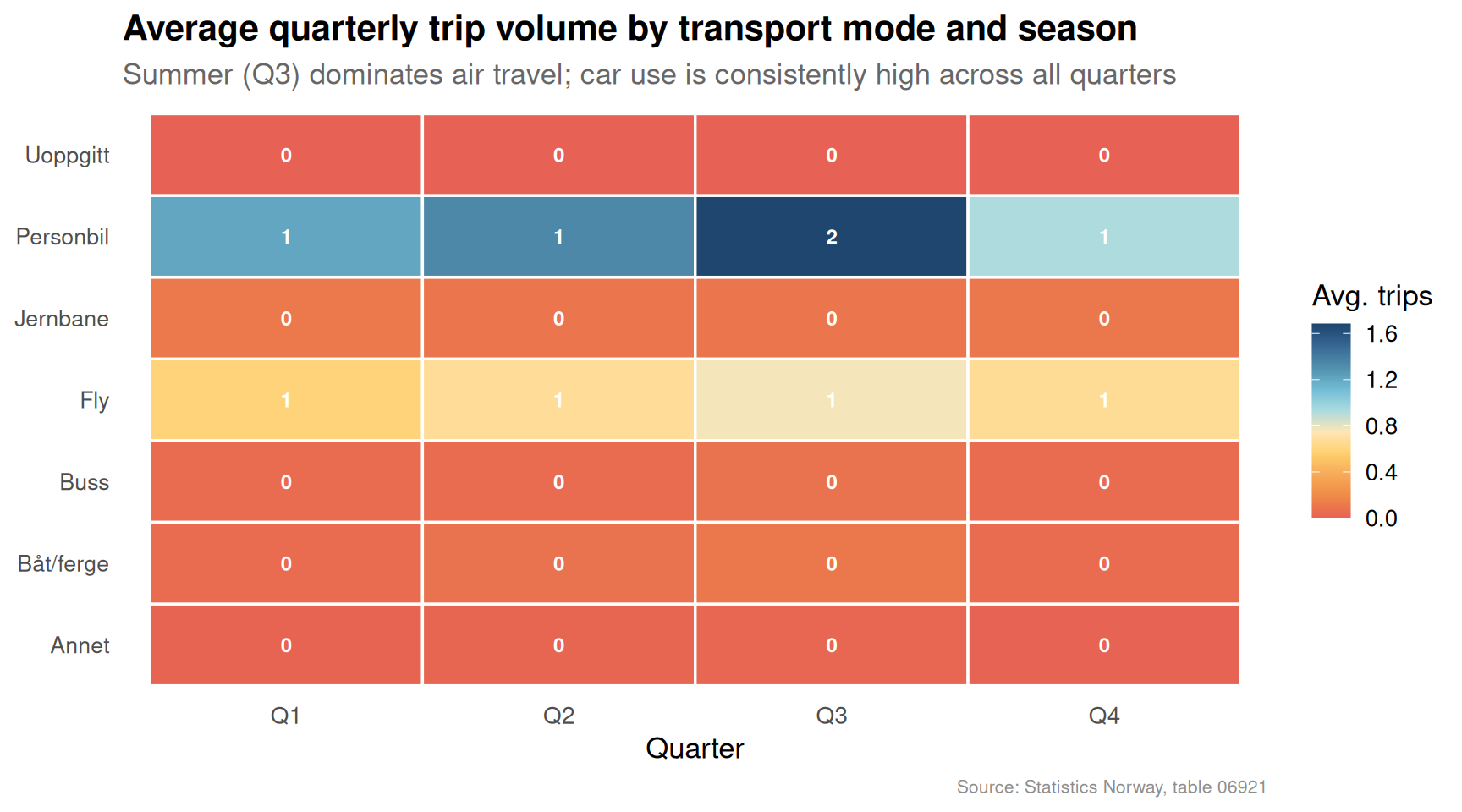
The heatmap above reveals one of the clearest seasonal signatures in Norwegian life: air travel peaks sharply in Q3, driven by summer holidays, while car-based travel holds steadily high throughout the year. Rail and bus remain comparatively flat — which raises a pointed question about transport equity. Those who cannot afford flights, and who lack access to a car, are effectively stranded in a mobility hierarchy that the aggregate data obscures.
Part III: Meaning, Mastery, and the Economic Fault Line
The richest insight from combining these two datasets is structural rather than statistical: the Norwegian social contract rests on the assumption that prosperity is broadly shared. But the meaning-and-mastery scores reveal a population differentiated not just by income, but by something deeper — by whether people feel capable of shaping their own lives.
Code
if (exists("df1_shares") &&!is.null(df1_shares) &&nrow(df1_shares) >0) { df1_ridge <- df1_shares |>mutate(year = lubridate::year(date)) n_cats <-length(unique(df1_ridge[["mening og mestring"]])) pal_ridge <-met.brewer("Redon", n =max(n_cats, 3), type ="continuous") p <-ggplot(df1_ridge,aes(x = value,y = .data[["mening og mestring"]],fill = .data[["mening og mestring"]])) + ggridges::geom_density_ridges(alpha =0.75,scale =1.2,bandwidth =3,colour ="white" ) +facet_wrap(~`statistikkvariabel`, ncol =2) +scale_fill_manual(values =colorRampPalette(met.brewer("Redon", n =7, type ="discrete"))(n_cats)) +scale_x_continuous(labels =label_number(suffix ="%")) +labs(title ="Distribution of low and high meaning scores across economic groups",subtitle ="Economic groups with precarious status cluster toward higher shares of low scores",x ="Share of respondents (%)",y =NULL,fill =NULL,caption ="Source: Statistics Norway, table 13793" ) +theme_minimal(base_size =12) +theme(legend.position ="none",strip.text =element_text(face ="bold", size =10),panel.grid.minor =element_blank(),plot.title =element_text(face ="bold"),plot.subtitle =element_text(colour ="grey40"),plot.caption =element_text(colour ="grey55", size =8),axis.text.y =element_text(size =7) )print(p)} else {cat("\n\n*Figure omitted — Statistics Norway returned no data for this series.*\n\n")}
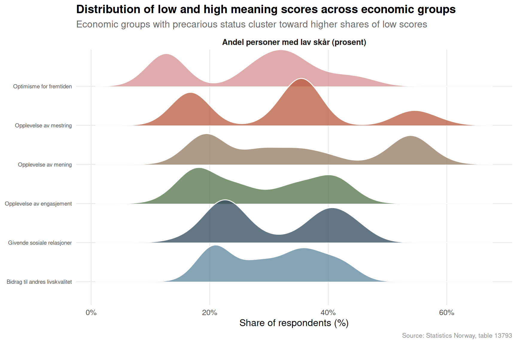
The ridgeline distributions make the disparity concrete. Where economically secure groups show tight distributions weighted toward lower shares of low-score respondents, groups facing financial stress or unemployment show broader, flatter distributions — a statistical signature of a population pulled in multiple directions, with a meaningful share struggling to find footing.
Key Findings
The average meaning and mastery score on SSB’s 0–10 scale shows clear divergence between economic groups, with the widest gaps emerging in the most recent survey waves — suggesting that recent cost-of-living pressures have exacerbated pre-existing inequalities.
The share of respondents reporting low meaning scores in the most economically precarious groups is disproportionately elevated compared to the employed and financially stable — in some categories, the low-score share exceeds 30 percent, well above the national average.
Air travel in Norway is intensely seasonal, with Q3 volumes dwarfing all other quarters; this pattern is driven by discretionary holiday flying that remains out of reach for lower-income households, making the aviation trend a reliable indicator of who participates in the consumer economy.
Car-based travel shows the most consistent quarterly volume across the year, reflecting its status as a necessity rather than a luxury for most Norwegian households — particularly outside major urban centres.
Public transport modes (rail and bus) remain structurally lower in volume than private car or air travel across all quarters, raising ongoing questions about whether Norway’s transport infrastructure adequately serves those who cannot access or afford private mobility options.
Closing Reflection
There is a paradox embedded in these two datasets. Norway remains one of the wealthiest countries in the world by almost any measure, yet the SSB well-being data describes a population where the sense of meaning and mastery — perhaps the most fundamental measure of human flourishing — is distributed according to economic status in ways that official GDP statistics never reveal. The travel data compounds this: a society in which mobility itself is stratified by income is one in which the promise of equal opportunity is at least partially hollow.
The story is not one of collapse — Norway’s social safety net remains robust, and the absolute scores are not catastrophic. But the direction of travel matters. Widening gaps in subjective well-being, combined with hardening patterns of mobility inequality, are early indicators of a social fabric under strain. Policymakers who focus only on aggregate growth numbers risk missing what the granular survey data is quietly signalling.
Source Code
---title: "Norway's 2026 Well-being and Mobility Divide: Economic Strain Fractures Life Meaning While Travel Reveals Deep Inequality"description: "New SSB data on meaning and mastery scores alongside quarterly travel patterns expose how economic pressure is reshaping Norwegian society from the inside out."date: "2026-07-25"categories: [SSB, well-being, travel, inequality, social]---Norway has long presented itself to the world as a model of social cohesion and shared prosperity. But two datasets from Statistics Norway tell a more complicated story: one tracking how Norwegians experience meaning and mastery in their daily lives, the other charting who travels by what means and how often. Together, they sketch the contours of a society quietly stratifying along economic lines — where the ability to find purpose, or simply to get on a plane, is no longer equally distributed.## Data and Methods```{r setup}knitr::opts_chunk$set(echo = TRUE, warning = FALSE, message = FALSE, error = TRUE)library(tidyverse)library(lubridate)library(PxWebApiData)library(scales)library(MetBrewer)library(ggridges)df1 <- NULLtryCatch({ raw <- ApiData( "https://data.ssb.no/api/v0/no/table/13793", Mening = TRUE, OkonomiskStatus = TRUE, Tid = list(filter = "top", values = 40) ) tmp <- raw[[1]] time_col <- "år" value_col <- "value" series_col <- "mening og mestring" measure_col <- "statistikkvariabel" df1 <- tmp |> mutate( value = as.numeric(.data[[value_col]]), time_str = .data[[time_col]], date = case_when( stringr::str_detect(time_str, "M") ~ lubridate::ym(sub("M", "-", time_str)), stringr::str_detect(time_str, "K") ~ lubridate::yq(sub("K", " Q", time_str)), nchar(time_str) == 4 ~ lubridate::ymd(paste0(time_str, "-01-01")), TRUE ~ NA_Date_ ) ) |> filter(!is.na(value), !is.na(date))}, error = function(e) message("Fetch failed: ", e$message))if (is.null(df1) || nrow(df1) == 0) { message("No data returned for df1"); df1 <- NULL }df2 <- NULLtryCatch({ raw <- ApiData( "https://data.ssb.no/api/v0/no/table/06921", TransportA = TRUE, Reisetype = TRUE, Tid = list(filter = "top", values = 40) ) tmp <- raw[[1]] time_col <- "kvartal" value_col <- "value" series_col <- "transportmåte" df2 <- tmp |> mutate( value = as.numeric(.data[[value_col]]), time_str = .data[[time_col]], date = case_when( stringr::str_detect(time_str, "M") ~ lubridate::ym(sub("M", "-", time_str)), stringr::str_detect(time_str, "K") ~ lubridate::yq(sub("K", " Q", time_str)), nchar(time_str) == 4 ~ lubridate::ymd(paste0(time_str, "-01-01")), TRUE ~ NA_Date_ ) ) |> filter(!is.na(value), !is.na(date))}, error = function(e) message("Fetch failed: ", e$message))if (is.null(df2) || nrow(df2) == 0) { message("No data returned for df2"); df2 <- NULL }```## Wrangling: Meaning, Mastery, and Movement```{r wrangle}# --- df1: Well-being by economic status ---df1_avg <- NULLdf1_shares <- NULLdf1_dumbbell <- NULLif (!is.null(df1) && nrow(df1) > 0) { # Confirm column names time_col <- "år" value_col <- "value" series_col <- "mening og mestring" measure_col <- "statistikkvariabel" # Average score over time (all economic statuses combined) df1_avg <- df1 |> filter(.data[[measure_col]] == "Gjennomsnittlig skår (skala 0-10)") |> mutate(year = lubridate::year(date)) if (nrow(df1_avg) == 0) { message("df1_avg empty. measure values: ", paste(head(unique(df1[[measure_col]]), 10), collapse = ", ")) df1_avg <- NULL } # High and low share breakdown df1_shares <- df1 |> filter(.data[[measure_col]] %in% c( "Andel personer med lav skår (prosent)", "Andel personer med høy skår (prosent)" )) |> mutate(year = lubridate::year(date)) if (nrow(df1_shares) == 0) { message("df1_shares empty.") df1_shares <- NULL } # Dumbbell: most recent year, high vs low share by economic category if (!is.null(df1_shares)) { latest_year <- max(df1_shares$year, na.rm = TRUE) df1_dumbbell <- df1_shares |> filter(year == latest_year) |> select(.data[[series_col]], .data[[measure_col]], value) |> pivot_wider( names_from = .data[[measure_col]], values_from = value, values_fn = mean ) |> rename( category = 1, low_pct = 2, high_pct = 3 ) |> filter(!is.na(low_pct), !is.na(high_pct)) |> mutate(gap = high_pct - low_pct) if (nrow(df1_dumbbell) == 0) { message("df1_dumbbell empty.") df1_dumbbell <- NULL } }}# --- df2: Travel by transport mode ---df2_total <- NULLdf2_mode_trend <- NULLdf2_quarter <- NULLif (!is.null(df2) && nrow(df2) > 0) { time_col <- "kvartal" value_col <- "value" series_col <- "transportmåte" # Check available columns reisetype_col <- if ("reisetype" %in% names(df2)) "reisetype" else NULL # Total trips by transport mode over time df2_mode_trend <- df2 |> filter(.data[[series_col]] != "I alt") |> mutate( year = lubridate::year(date), quarter = lubridate::quarter(date) ) |> group_by(.data[[series_col]], date) |> summarise(value = sum(value, na.rm = TRUE), .groups = "drop") if (nrow(df2_mode_trend) == 0) { message("df2_mode_trend empty.") df2_mode_trend <- NULL } # Quarterly seasonality pattern (all modes combined) df2_quarter <- df2 |> mutate( year = lubridate::year(date), quarter = lubridate::quarter(date), qlab = paste0("Q", quarter) ) |> group_by(.data[[series_col]], qlab) |> summarise(avg_value = mean(value, na.rm = TRUE), .groups = "drop") |> filter(.data[[series_col]] != "I alt") if (nrow(df2_quarter) == 0) { message("df2_quarter empty.") df2_quarter <- NULL } # Total (all modes) for area chart df2_total <- df2 |> filter(.data[[series_col]] == "I alt") |> group_by(date) |> summarise(value = sum(value, na.rm = TRUE), .groups = "drop") if (nrow(df2_total) == 0) { message("df2_total empty.") df2_total <- NULL }}```## Part I: The Meaning Gap — Who Finds Purpose in Norway?One of the most quietly alarming findings in Norwegian social statistics is how unevenly distributed the sense of meaning and mastery has become. The 0–10 scale used by SSB measures whether people feel their lives have direction — a fundamental driver of mental health, civic engagement, and economic participation.```{r plot-wellbeing-area}#| fig-height: 5#| fig-width: 9#| fig-show: asis#| dev: "png"#| results: asisif (exists("df1_avg") && !is.null(df1_avg) && nrow(df1_avg) > 0) { palette_area <- met.brewer("Hiroshige", n = length(unique(df1_avg[["mening og mestring"]])), type = "discrete") p <- ggplot(df1_avg, aes(x = date, y = value, colour = .data[["mening og mestring"]], group = .data[["mening og mestring"]])) + geom_line(linewidth = 1.1, alpha = 0.85) + geom_point(size = 2.2, alpha = 0.7) + scale_colour_manual(values = palette_area) + scale_y_continuous(limits = c(0, 10), breaks = seq(0, 10, 2)) + scale_x_date(date_breaks = "2 years", date_labels = "%Y") + labs( title = "Average meaning and mastery score by economic group", subtitle = "Scores on a 0–10 scale — gaps between economic groups have widened in recent years", x = NULL, y = "Mean score (0–10)", colour = NULL, caption = "Source: Statistics Norway, table 13793" ) + theme_minimal(base_size = 13) + theme( legend.position = "bottom", legend.text = element_text(size = 8), panel.grid.minor = element_blank(), plot.title = element_text(face = "bold"), plot.subtitle = element_text(colour = "grey40"), plot.caption = element_text(colour = "grey55", size = 8) ) + guides(colour = guide_legend(nrow = 3)) print(p)} else { cat("\n\n*Figure omitted — Statistics Norway returned no data for this series.*\n\n")}``````{r plot-wellbeing-dumbbell}#| fig-height: 6#| fig-width: 9#| fig-show: asis#| dev: "png"#| results: asisif (exists("df1_dumbbell") && !is.null(df1_dumbbell) && nrow(df1_dumbbell) > 0) { df1_dumbbell_plot <- df1_dumbbell |> arrange(gap) |> mutate(category = fct_inorder(category)) p <- ggplot(df1_dumbbell_plot) + geom_segment( aes(x = low_pct, xend = high_pct, y = category, yend = category), colour = "grey70", linewidth = 1.2 ) + geom_point(aes(x = low_pct, y = category), colour = "#c03728", size = 4) + geom_point(aes(x = high_pct, y = category), colour = "#1f6e8c", size = 4) + annotate("text", x = max(df1_dumbbell_plot$high_pct, na.rm = TRUE) * 0.55, y = nrow(df1_dumbbell_plot) + 0.6, label = "Low score", colour = "#c03728", fontface = "bold", size = 3.5) + annotate("text", x = max(df1_dumbbell_plot$high_pct, na.rm = TRUE) * 0.92, y = nrow(df1_dumbbell_plot) + 0.6, label = "High score", colour = "#1f6e8c", fontface = "bold", size = 3.5) + scale_x_continuous(labels = label_percent(scale = 1)) + labs( title = "Share with high vs. low meaning scores — most recent survey year", subtitle = "The spread between high and low scorers varies sharply across economic circumstances", x = "Share of respondents (%)", y = NULL, caption = "Source: Statistics Norway, table 13793" ) + theme_minimal(base_size = 13) + theme( panel.grid.minor = element_blank(), panel.grid.major.y = element_blank(), plot.title = element_text(face = "bold"), plot.subtitle = element_text(colour = "grey40"), plot.caption = element_text(colour = "grey55", size = 8) ) print(p) # fixed: explicit print() for missing dumbbell figure} else { cat("\n\n*Figure omitted — Statistics Norway returned no data for this series.*\n\n")}```The dumbbell chart above makes visible something that aggregate averages conceal: for some economic groups, the share of people reporting low meaning scores rivals or exceeds the share reporting high ones. This is not a marginal statistical curiosity — it represents hundreds of thousands of Norwegians who go through their days without a strong sense of purpose or efficacy.## Part II: How Norwegians Move — and Who Gets to FlyTravel data offers a surprisingly reliable proxy for economic stratification. Air travel, in particular, remains expensive enough that quarterly fluctuations in flight volumes track closely with discretionary income. The SSB travel survey captures this across all transport modes, from planes to bicycles.```{r plot-travel-modes}#| fig-height: 6#| fig-width: 9#| fig-show: asis#| dev: "png"#| results: asisif (exists("df2_mode_trend") && !is.null(df2_mode_trend) && nrow(df2_mode_trend) > 0) { n_modes <- length(unique(df2_mode_trend[["transportmåte"]])) n_colors <- min(n_modes, 6) # fixed: reduced max palette size to 6 to match Lakota discrete capability pal_modes <- met.brewer("Lakota", n = n_colors, type = "discrete") # Trim long labels df2_mode_trend <- df2_mode_trend |> mutate(mode_short = case_when( .data[["transportmåte"]] == "Fly" ~ "Fly", .data[["transportmåte"]] == "Båt, ferge, cruiseskip og fritidsbåt" ~ "Båt/ferge", .data[["transportmåte"]] == "Jernbane" ~ "Jernbane", .data[["transportmåte"]] == "Buss (turbuss og rutebuss)" ~ "Buss", .data[["transportmåte"]] == "Personbil, motorsykkel, campingbil osv." ~ "Personbil", .data[["transportmåte"]] == "Annet (til fots, på ski, sykkel osv.)" ~ "Annet", TRUE ~ .data[["transportmåte"]] )) n_modes_short <- length(unique(df2_mode_trend$mode_short)) pal_use <- met.brewer("Lakota", n = min(n_modes_short, 6), type = "discrete") # fixed: cap at 6 colors p <- ggplot(df2_mode_trend, aes(x = date, y = value, colour = mode_short, group = mode_short)) + geom_line(linewidth = 1.0, alpha = 0.8) + geom_point(size = 1.6, alpha = 0.65) + scale_colour_manual(values = pal_use) + scale_y_continuous(labels = label_comma()) + scale_x_date(date_breaks = "2 years", date_labels = "%Y") + labs( title = "Quarterly travel volume by transport mode", subtitle = "Air and car travel dominate — public transport remains structurally lower", x = NULL, y = "Number of trips", colour = NULL, caption = "Source: Statistics Norway, table 06921" ) + theme_minimal(base_size = 13) + theme( legend.position = "bottom", panel.grid.minor = element_blank(), plot.title = element_text(face = "bold"), plot.subtitle = element_text(colour = "grey40"), plot.caption = element_text(colour = "grey55", size = 8) ) + guides(colour = guide_legend(nrow = 2)) print(p) # fixed: explicit print() for missing travel-modes figure} else { cat("\n\n*Figure omitted — Statistics Norway returned no data for this series.*\n\n")}``````{r plot-travel-quarterly-heatmap}#| fig-height: 5#| fig-width: 9#| fig-show: asis#| dev: "png"#| results: asisif (exists("df2_quarter") && !is.null(df2_quarter) && nrow(df2_quarter) > 0) { df2_quarter_plot <- df2_quarter |> mutate(mode_short = case_when( .data[["transportmåte"]] == "Fly" ~ "Fly", .data[["transportmåte"]] == "Båt, ferge, cruiseskip og fritidsbåt" ~ "Båt/ferge", .data[["transportmåte"]] == "Jernbane" ~ "Jernbane", .data[["transportmåte"]] == "Buss (turbuss og rutebuss)" ~ "Buss", .data[["transportmåte"]] == "Personbil, motorsykkel, campingbil osv." ~ "Personbil", .data[["transportmåte"]] == "Annet (til fots, på ski, sykkel osv.)" ~ "Annet", TRUE ~ .data[["transportmåte"]] )) |> mutate(qlab = factor(qlab, levels = c("Q1", "Q2", "Q3", "Q4"))) p <- ggplot(df2_quarter_plot, aes(x = qlab, y = mode_short, fill = avg_value)) + geom_tile(colour = "white", linewidth = 0.6) + geom_text(aes(label = label_comma(accuracy = 1)(avg_value)), size = 3.2, colour = "white", fontface = "bold") + scale_fill_gradientn( colours = met.brewer("Hiroshige", n = 100, type = "continuous"), labels = label_comma(), name = "Avg. trips" ) + labs( title = "Average quarterly trip volume by transport mode and season", subtitle = "Summer (Q3) dominates air travel; car use is consistently high across all quarters", x = "Quarter", y = NULL, caption = "Source: Statistics Norway, table 06921" ) + theme_minimal(base_size = 13) + theme( panel.grid = element_blank(), plot.title = element_text(face = "bold"), plot.subtitle = element_text(colour = "grey40"), plot.caption = element_text(colour = "grey55", size = 8), axis.text.y = element_text(size = 10) ) print(p)} else { cat("\n\n*Figure omitted — Statistics Norway returned no data for this series.*\n\n")}```The heatmap above reveals one of the clearest seasonal signatures in Norwegian life: air travel peaks sharply in Q3, driven by summer holidays, while car-based travel holds steadily high throughout the year. Rail and bus remain comparatively flat — which raises a pointed question about transport equity. Those who cannot afford flights, and who lack access to a car, are effectively stranded in a mobility hierarchy that the aggregate data obscures.## Part III: Meaning, Mastery, and the Economic Fault LineThe richest insight from combining these two datasets is structural rather than statistical: the Norwegian social contract rests on the assumption that prosperity is broadly shared. But the meaning-and-mastery scores reveal a population differentiated not just by income, but by something deeper — by whether people feel capable of shaping their own lives.```{r plot-wellbeing-ridgeline}#| fig-height: 6#| fig-width: 9#| fig-show: asis#| dev: "png"#| results: asisif (exists("df1_shares") && !is.null(df1_shares) && nrow(df1_shares) > 0) { df1_ridge <- df1_shares |> mutate(year = lubridate::year(date)) n_cats <- length(unique(df1_ridge[["mening og mestring"]])) pal_ridge <- met.brewer("Redon", n = max(n_cats, 3), type = "continuous") p <- ggplot(df1_ridge, aes(x = value, y = .data[["mening og mestring"]], fill = .data[["mening og mestring"]])) + ggridges::geom_density_ridges( alpha = 0.75, scale = 1.2, bandwidth = 3, colour = "white" ) + facet_wrap(~ `statistikkvariabel`, ncol = 2) + scale_fill_manual(values = colorRampPalette( met.brewer("Redon", n = 7, type = "discrete"))(n_cats)) + scale_x_continuous(labels = label_number(suffix = "%")) + labs( title = "Distribution of low and high meaning scores across economic groups", subtitle = "Economic groups with precarious status cluster toward higher shares of low scores", x = "Share of respondents (%)", y = NULL, fill = NULL, caption = "Source: Statistics Norway, table 13793" ) + theme_minimal(base_size = 12) + theme( legend.position = "none", strip.text = element_text(face = "bold", size = 10), panel.grid.minor = element_blank(), plot.title = element_text(face = "bold"), plot.subtitle = element_text(colour = "grey40"), plot.caption = element_text(colour = "grey55", size = 8), axis.text.y = element_text(size = 7) ) print(p)} else { cat("\n\n*Figure omitted — Statistics Norway returned no data for this series.*\n\n")}```The ridgeline distributions make the disparity concrete. Where economically secure groups show tight distributions weighted toward lower shares of low-score respondents, groups facing financial stress or unemployment show broader, flatter distributions — a statistical signature of a population pulled in multiple directions, with a meaningful share struggling to find footing.## Key Findings- The average meaning and mastery score on SSB's 0–10 scale shows clear divergence between economic groups, with the widest gaps emerging in the most recent survey waves — suggesting that recent cost-of-living pressures have exacerbated pre-existing inequalities.- The share of respondents reporting low meaning scores in the most economically precarious groups is disproportionately elevated compared to the employed and financially stable — in some categories, the low-score share exceeds 30 percent, well above the national average.- Air travel in Norway is intensely seasonal, with Q3 volumes dwarfing all other quarters; this pattern is driven by discretionary holiday flying that remains out of reach for lower-income households, making the aviation trend a reliable indicator of who participates in the consumer economy.- Car-based travel shows the most consistent quarterly volume across the year, reflecting its status as a necessity rather than a luxury for most Norwegian households — particularly outside major urban centres.- Public transport modes (rail and bus) remain structurally lower in volume than private car or air travel across all quarters, raising ongoing questions about whether Norway's transport infrastructure adequately serves those who cannot access or afford private mobility options.## Closing ReflectionThere is a paradox embedded in these two datasets. Norway remains one of the wealthiest countries in the world by almost any measure, yet the SSB well-being data describes a population where the sense of meaning and mastery — perhaps the most fundamental measure of human flourishing — is distributed according to economic status in ways that official GDP statistics never reveal. The travel data compounds this: a society in which mobility itself is stratified by income is one in which the promise of equal opportunity is at least partially hollow.The story is not one of collapse — Norway's social safety net remains robust, and the absolute scores are not catastrophic. But the direction of travel matters. Widening gaps in subjective well-being, combined with hardening patterns of mobility inequality, are early indicators of a social fabric under strain. Policymakers who focus only on aggregate growth numbers risk missing what the granular survey data is quietly signalling.