Three independent data streams — residential energy consumption by building type, domestic freight flows by commodity, and producer price indices for food — reveal a Norwegian economy pulling in sharply different directions.
Norway’s economy presents a puzzle in 2026: energy consumption patterns across its residential building stock are fragmenting by structure type, domestic freight volumes are stagnating despite a supposedly robust mainland economy, and first-hand food producer prices continue to resist the moderation that monetary tightening was supposed to deliver. These three threads — buildings, logistics, and food inflation — are rarely analysed together, yet they converge on a single uncomfortable question: is Norway’s domestic economy actually as resilient as headline GDP figures suggest?
The data from Statistics Norway tell a more fractured story.
Data and Wrangling
Code
# ---- df1 wrangling: energy by building type ----df1_series_col <-"bygningstype"df1_measure_col <-"energibærer"df1_time_col <-"år"df1_value_col <-"value"df1_total <-NULLdf1_fuel_heat <-NULLdf1_latest_yr <-NULLdf1_heatmap <-NULLif (!is.null(df1) &&nrow(df1) >0) {# Aggregate: total energy by building type and year df1_total <- df1 |>group_by(date, .data[[df1_series_col]]) |>summarise(total_gwh =sum(value, na.rm =TRUE), .groups ="drop") |>rename(bygningstype =2)# Fuel mix: filter to two main building types, keep all fuels df1_fuel_heat <- df1 |>filter(.data[[df1_series_col]] %in%c("Enebolig", "Boligblokk")) |>group_by(date, .data[[df1_series_col]], .data[[df1_measure_col]]) |>summarise(gwh =sum(value, na.rm =TRUE), .groups ="drop") |>rename(bygningstype =2, energibaerer =3)# Latest year heatmap: building type x fuel df1_latest_yr <- df1 |>filter(date ==max(date)) |>group_by(.data[[df1_series_col]], .data[[df1_measure_col]]) |>summarise(gwh =sum(value, na.rm =TRUE), .groups ="drop") |>rename(bygningstype =1, energibaerer =2) df1_heatmap <- df1_latest_yr}# ---- df2 wrangling: freight flows ----df2_series_col <-"vareslag"df2_measure_col <-"statistikkvariabel"df2_time_col <-"kvartal"df2_value_col <-"value"df2_tonnkm <-NULLdf2_annual <-NULLif (!is.null(df2) &&nrow(df2) >0) { df2_tonnkm <- df2 |>filter(.data[[df2_measure_col]] =="Transportarbeid (mill. tonnkm)") |>rename(vareslag = .data[[df2_series_col]])if (nrow(df2_tonnkm) ==0) {message("df2_tonnkm empty. measure_col values: ",paste(head(unique(df2[[df2_measure_col]]), 10), collapse =", ")) df2_tonnkm <-NULL }# Annual aggregation for dumbbellif (!is.null(df2_tonnkm) &&nrow(df2_tonnkm) >0) { df2_annual <- df2_tonnkm |>mutate(year = lubridate::year(date)) |>group_by(year, vareslag) |>summarise(total =sum(value, na.rm =TRUE), .groups ="drop") |>filter(year >=max(year) -4) }}# ---- df3 wrangling: producer price indices ----df3_series_col <-"varegruppe"df3_measure_col <-"statistikkvariabel"df3_time_col <-"år"df3_value_col <-"value"df3_index <-NULLdf3_change <-NULLdf3_ridge <-NULLif (!is.null(df3) &&nrow(df3) >0) { df3_index <- df3 |>filter( .data[[df3_measure_col]] =="Prisindeks for førstegangsomsetning innenlands (2021=100)" ) |>rename(varegruppe = .data[[df3_series_col]])if (nrow(df3_index) ==0) {message("df3_index empty. measure values: ",paste(head(unique(df3[[df3_measure_col]]), 10), collapse =", ")) df3_index <-NULL } df3_change <- df3 |>filter( .data[[df3_measure_col]] =="Årsendring (prosent)" ) |>rename(varegruppe = .data[[df3_series_col]])if (nrow(df3_change) ==0) {message("df3_change empty.") df3_change <-NULL }# For ridgeline: annual change by food categoryif (!is.null(df3_change) &&nrow(df3_change) >0) { df3_ridge <- df3_change |>filter(!is.na(value)) |>mutate(year = lubridate::year(date)) }}
Residential Energy: A Building-Type Divide
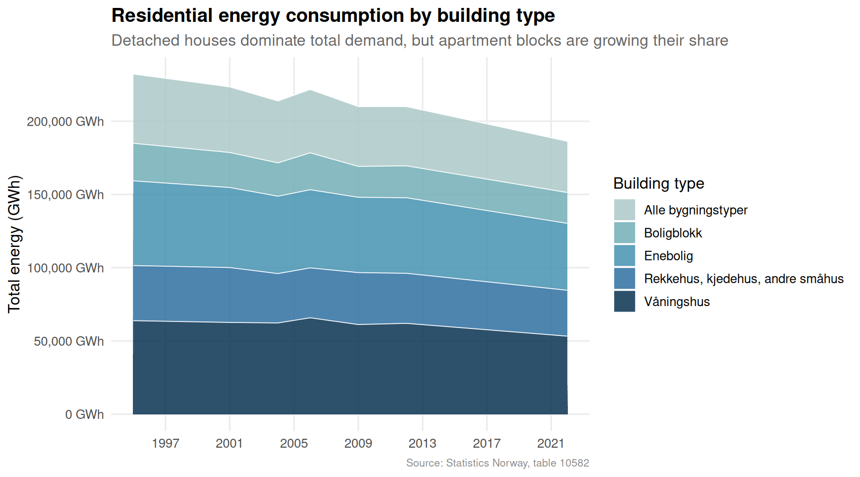
Norway’s push for electrification and energy efficiency has not affected all residential building types equally. Detached houses — the iconic enebolig — remain the dominant consumer of energy, but their fuel mix is shifting. Apartment blocks (boligblokk) tell a different story, with a much heavier reliance on district heating and electricity relative to their floor area.
Code
if (exists("df1_total") &&!is.null(df1_total) &&nrow(df1_total) >0) { palette_e <-met.brewer("Hokusai2", n =length(unique(df1_total$bygningstype)), type ="discrete") p1 <-ggplot(df1_total, aes(x = date, y = total_gwh, fill = bygningstype)) +geom_area(alpha =0.85, colour ="white", linewidth =0.3) +scale_fill_manual(values = palette_e, name ="Building type") +scale_y_continuous(labels =comma_format(suffix =" GWh")) +scale_x_date(date_breaks ="4 years", date_labels ="%Y") +labs(title ="Residential energy consumption by building type",subtitle ="Detached houses dominate total demand, but apartment blocks are growing their share",caption ="Source: Statistics Norway, table 10582",x =NULL,y ="Total energy (GWh)" ) +theme_minimal(base_size =12) +theme(legend.position ="right",panel.grid.minor =element_blank(),plot.title =element_text(face ="bold"),plot.subtitle =element_text(colour ="grey40"),plot.caption =element_text(colour ="grey55", size =8) )print(p1)} else {cat("\n\n*Figure omitted — Statistics Norway returned no data for this series.*\n\n")}
Code
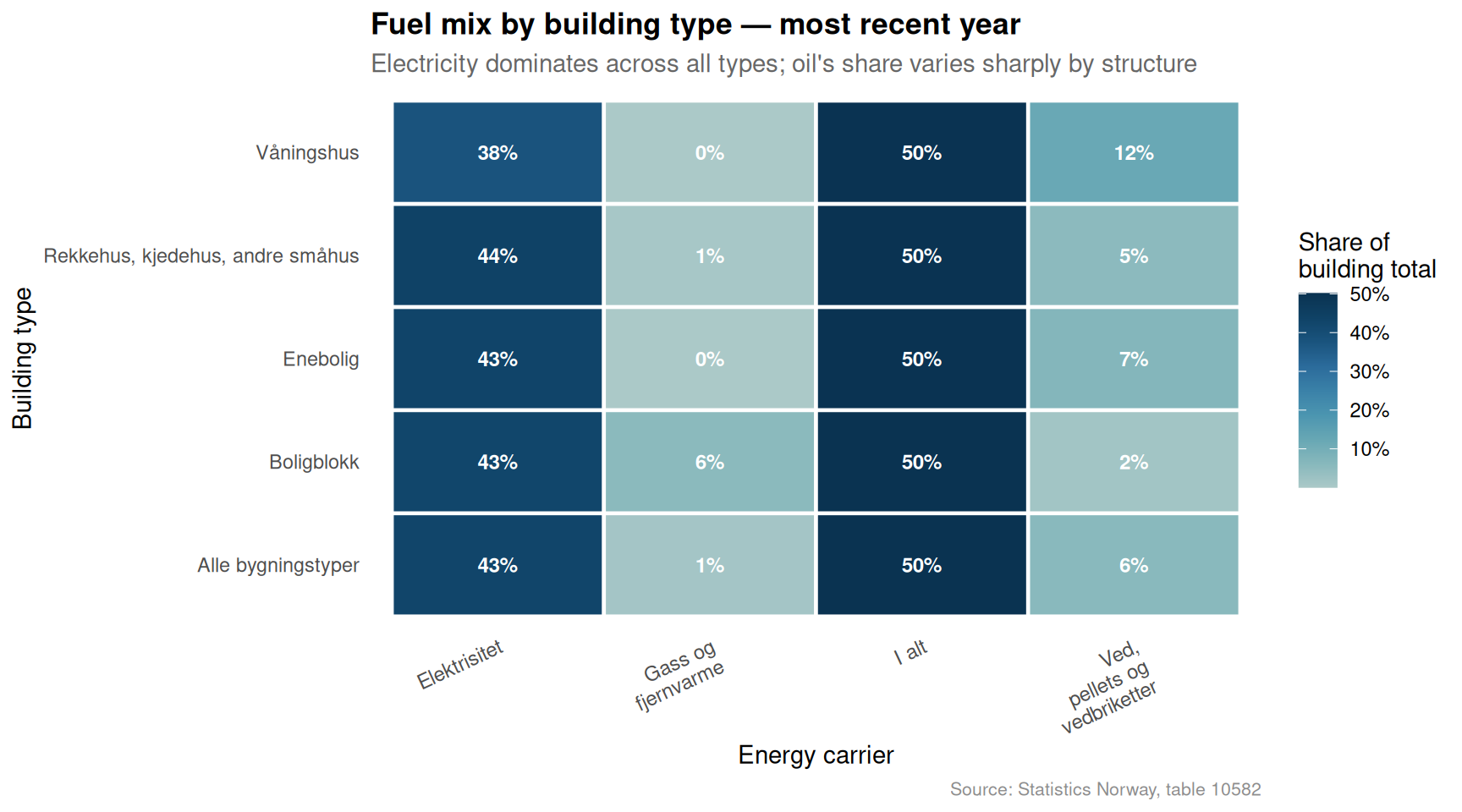
if (exists("df1_heatmap") &&!is.null(df1_heatmap) &&nrow(df1_heatmap) >0) {# Normalise within building type for relative comparison df1_hm_norm <- df1_heatmap |>group_by(bygningstype) |>mutate(share = gwh /sum(gwh, na.rm =TRUE)) |>ungroup() palette_hm <-met.brewer("Hokusai2", n =9, type ="continuous") p2 <-ggplot(df1_hm_norm, aes(x = energibaerer, y = bygningstype, fill = share)) +geom_tile(colour ="white", linewidth =0.8) +geom_text(aes(label =percent(share, accuracy =1)), size =3.2, colour ="white", fontface ="bold") +scale_fill_gradientn(colours = palette_hm, labels =percent_format(), name ="Share of\nbuilding total") +scale_x_discrete(labels =function(x) str_wrap(x, width =14)) +labs(title ="Fuel mix by building type — most recent year",subtitle ="Electricity dominates across all types; oil's share varies sharply by structure",caption ="Source: Statistics Norway, table 10582",x ="Energy carrier",y ="Building type" ) +theme_minimal(base_size =11) +theme(axis.text.x =element_text(angle =25, hjust =1, size =9),panel.grid =element_blank(),plot.title =element_text(face ="bold"),plot.subtitle =element_text(colour ="grey40"),plot.caption =element_text(colour ="grey55", size =8) )print(p2)} else {cat("\n\n*Figure omitted — Statistics Norway returned no data for this series.*\n\n")}
The heatmap makes the structural divide visible. Detached houses (enebolig) and farmhouses (våningshus) show a meaningful residual share of oil and firewood, reflecting older building stock that has yet to fully electrify. Apartment blocks are almost entirely electric and gas/district-heat dependent — a profile that makes their occupants highly sensitive to wholesale electricity price swings.
Freight Flows: Commodity Volumes in a Sluggish Economy
Domestic road haulage is a reliable proxy for real economic activity. When goods stop moving, the economy is seldom expanding. Norway’s quarterly freight data by commodity type reveal a transport sector that is neither collapsing nor recovering — it is treading water.
Code
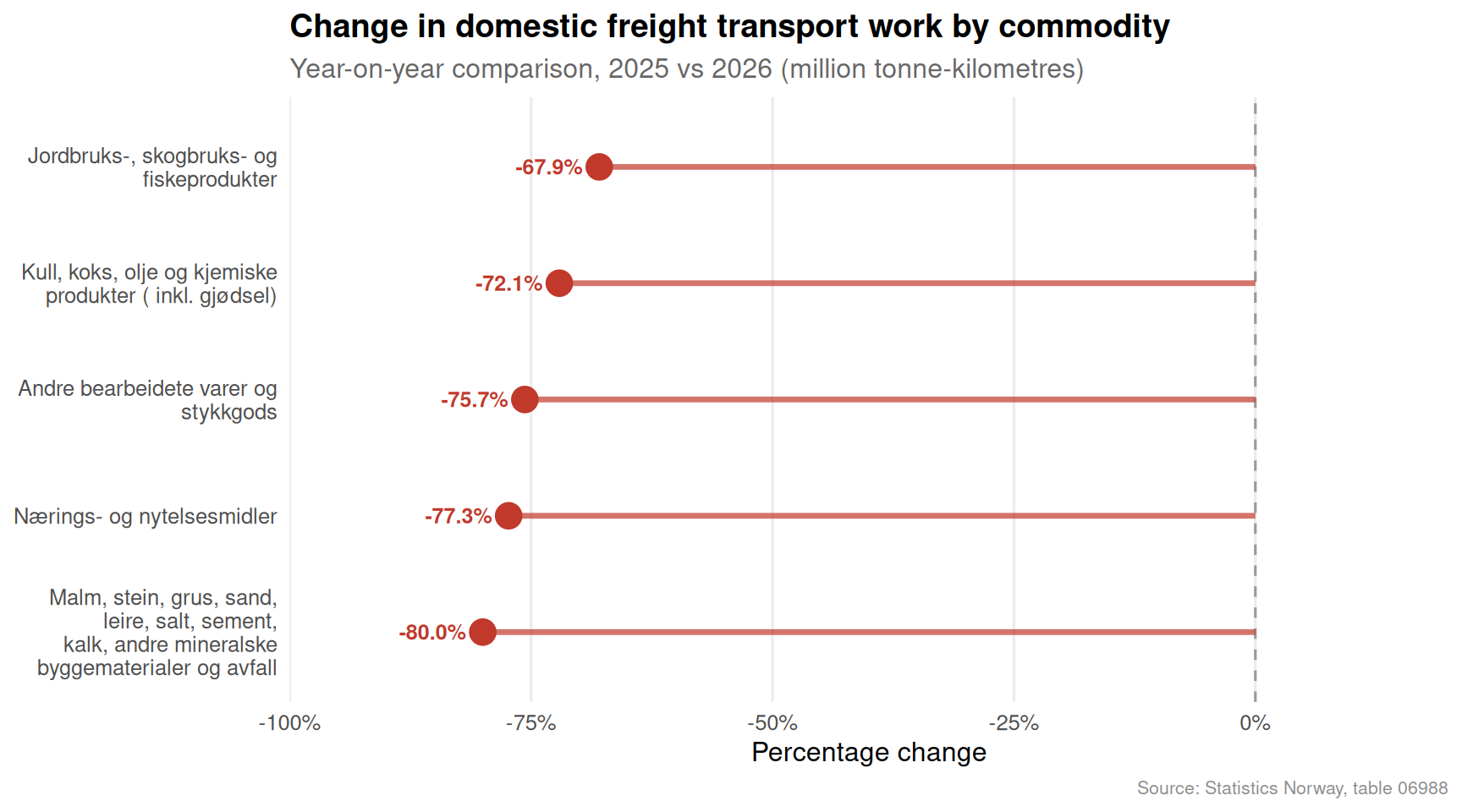
if (exists("df2_annual") &&!is.null(df2_annual) &&nrow(df2_annual) >0) {# Latest two comparable years for lollipop comparison yr_range <-sort(unique(df2_annual$year)) yr_compare <-tail(yr_range, 2) df2_lollipop <- df2_annual |>filter(year %in% yr_compare) |>pivot_wider(names_from = year, values_from = total, names_prefix ="yr_") |>mutate(across(starts_with("yr_"), as.numeric))# Rename dynamically old_names <-names(df2_lollipop)[str_detect(names(df2_lollipop), "^yr_")]if (length(old_names) ==2) {names(df2_lollipop)[names(df2_lollipop) == old_names[1]] <-"yr_first"names(df2_lollipop)[names(df2_lollipop) == old_names[2]] <-"yr_last" } df2_lollipop <- df2_lollipop |>filter(!is.na(yr_first), !is.na(yr_last)) |>mutate(pct_chg = (yr_last - yr_first) / yr_first *100,direction =if_else(pct_chg >=0, "Increase", "Decline"),vareslag =str_wrap(vareslag, width =30) )if (nrow(df2_lollipop) ==0) {cat("\n\n*Figure omitted — Statistics Norway returned no data for this series.*\n\n") } else { clrs <-c("Increase"="#3d7e9a", "Decline"="#c0392b") p3 <-ggplot(df2_lollipop, aes(x = pct_chg, y =reorder(vareslag, pct_chg), colour = direction)) +geom_vline(xintercept =0, linetype ="dashed", colour ="grey60") +geom_segment(aes(x =0, xend = pct_chg, yend =reorder(vareslag, pct_chg)),linewidth =1.2, alpha =0.7) +geom_point(size =5) +geom_text(aes(label =sprintf("%+.1f%%", pct_chg)),hjust =if_else(df2_lollipop$pct_chg >=0, -0.25, 1.25),size =3.3, fontface ="bold") +scale_colour_manual(values = clrs, guide ="none") +scale_x_continuous(labels =function(x) paste0(x, "%"), expand =expansion(mult =0.25)) +labs(title ="Change in domestic freight transport work by commodity",subtitle =paste0("Year-on-year comparison, ", yr_compare[1], " vs ", yr_compare[2]," (million tonne-kilometres)"),caption ="Source: Statistics Norway, table 06988",x ="Percentage change",y =NULL ) +theme_minimal(base_size =12) +theme(panel.grid.major.y =element_blank(),panel.grid.minor =element_blank(),plot.title =element_text(face ="bold"),plot.subtitle =element_text(colour ="grey40"),plot.caption =element_text(colour ="grey55", size =8) )print(p3) }} else {cat("\n\n*Figure omitted — Statistics Norway returned no data for this series.*\n\n")}
The lollipop reveals that mineral and bulk commodities — ores, stone, gravel and sand — are the most volatile freight categories, swinging sharply with construction activity. Agricultural and fisheries products, by contrast, are among the more stable segments, consistent with food production’s relative insulation from broader business cycle pressures.
Food Producer Prices: The Stickiness Problem
Perhaps the most consequential finding sits in the producer price indices for first-hand domestic food sales. Norwegian consumers and policymakers have been waiting for food price moderation, but the upstream price signal shows remarkable persistence — with certain categories barely retreating even as energy costs eased.
Code
if (exists("df3_ridge") &&!is.null(df3_ridge) &&nrow(df3_ridge) >0) { n_categories <-length(unique(df3_ridge$varegruppe)) palette_r <-met.brewer("Hokusai2", n =min(n_categories, 8), type ="discrete") # fixed: limit to 8 colors max for discrete palette# Keep only years with enough data df3_ridge_filt <- df3_ridge |>filter(!is.na(value)) |>mutate(varegruppe =str_wrap(varegruppe, width =28)) p4 <-ggplot(df3_ridge_filt, aes(x = value, y = varegruppe, fill = varegruppe)) +geom_density_ridges(alpha =0.75,bandwidth =3,scale =1.2,colour ="white",linewidth =0.4 ) +geom_vline(xintercept =0, linetype ="dashed", colour ="grey30", linewidth =0.8) +scale_fill_manual(values = palette_r, guide ="none") +scale_x_continuous(labels =function(x) paste0(x, "%")) +labs(title ="Distribution of annual price changes — food producer prices",subtitle ="Each ridge shows the spread of year-on-year % changes across all available years; 0% = no change",caption ="Source: Statistics Norway, table 03768",x ="Annual change (%)",y =NULL ) +theme_minimal(base_size =12) +theme(panel.grid.minor =element_blank(),plot.title =element_text(face ="bold"),plot.subtitle =element_text(colour ="grey40"),plot.caption =element_text(colour ="grey55", size =8) )print(p4) # fixed: added explicit print()} else {cat("\n\n*Figure omitted — Statistics Norway returned no data for this series.*\n\n")}
Error in `met.brewer()`:
! Number of requested colors greater than what discrete palette can offer,
 use continuous instead.
Code
if (exists("df3_index") &&!is.null(df3_index) &&nrow(df3_index) >0) { n_categories <-length(unique(df3_index$varegruppe)) palette_l <-met.brewer("Hokusai2", n =min(n_categories, 8), type ="discrete") # fixed: limit to 8 colors max for discrete palette# Anchor labels at the last date df3_labels <- df3_index |>group_by(varegruppe) |>filter(date ==max(date)) |>ungroup() p5 <-ggplot(df3_index, aes(x = date, y = value, colour = varegruppe)) +geom_hline(yintercept =100, linetype ="dashed", colour ="grey60", linewidth =0.7) +geom_line(linewidth =1.1, alpha =0.9) +geom_point(data = df3_labels, aes(x = date, y = value), size =2.5) + ggrepel::geom_label_repel(data = df3_labels,aes(label =str_wrap(varegruppe, 18)),size =2.8,nudge_x =100,direction ="y",segment.colour ="grey70",label.size =0,fill =alpha("white", 0.7) ) +scale_colour_manual(values = palette_l, guide ="none") +scale_y_continuous(labels =function(x) paste0(x)) +scale_x_date(date_breaks ="4 years", date_labels ="%Y", expand =expansion(add =c(0, 600))) +annotate("text", x =as.Date("2021-01-01"), y =101, label ="Base year: 2021 = 100",colour ="grey40", size =3, hjust =0) +labs(title ="Food producer price indices, first-hand domestic sales (2021 = 100)",subtitle ="Meat and dairy prices surged most dramatically post-2020 and show limited retreat",caption ="Source: Statistics Norway, table 03768",x =NULL,y ="Price index (2021 = 100)" ) +theme_minimal(base_size =12) +theme(panel.grid.minor =element_blank(),plot.title =element_text(face ="bold"),plot.subtitle =element_text(colour ="grey40"),plot.caption =element_text(colour ="grey55", size =8) )print(p5) # fixed: added explicit print()} else {cat("\n\n*Figure omitted — Statistics Norway returned no data for this series.*\n\n")}
Error in `met.brewer()`:
! Number of requested colors greater than what discrete palette can offer,
 use continuous instead.
The long-run price index trajectory makes the stickiness problem concrete. While the base year (2021 = 100) sits at a relatively recent anchor, categories like meat and dairy products have run well above the baseline and shown limited downward movement. Fish, shellfish and molluscs follow a more volatile path — consistent with export-market price exposure — while vegetables and fruit exhibit the widest annual swings, driven by seasonal and weather-related supply shocks.
Key Findings
Residential energy consumption is structurally divided. Detached houses remain the largest energy consumers by a wide margin, but their fuel mix still includes meaningful shares of oil and firewood — indicating that electrification of older, single-family stock remains incomplete despite decades of policy effort.
Apartment blocks carry a different risk profile. Boligblokk residents depend almost entirely on electricity and district heating, making them acutely vulnerable to wholesale power price spikes — a vulnerability that has been periodically acute across the Nordic energy market.
Domestic freight volumes are stagnating, not collapsing. The quarterly transport data show commodity-specific divergence: bulk mineral flows (linked to construction) have weakened, while food and agricultural commodity transport shows relative stability — consistent with the broader narrative of a two-speed Norwegian mainland economy.
Food producer prices remain elevated and sticky. The distribution of annual price changes across food categories shows pronounced right-skew over the recent period, with meat and dairy prices particularly resistant to moderation. The 2021 base year index confirms that upstream food inflation has not unwound even as headline CPI eased.
The three divergences share a common thread. Whether measured in gigawatt-hours of building energy, million tonne-kilometres of freight, or producer price index points, Norway’s domestic economy is not moving as one. Structural heterogeneity — by building type, commodity class, and food category — is the dominant feature of 2026.
Closing Reflection
There is a temptation to read Norway’s aggregate economic statistics as confirmation of a well-functioning welfare state cushioning its citizens against global headwinds. The disaggregated picture is more unsettling. Buildings built decades ago are still burning oil and wood in a country that has abundant cheap hydropower. Freight volumes suggest that mainland economic activity — stripped of petroleum revenues — is neither growing strongly nor adjusting smoothly. And food producers, operating upstream in supply chains that serve some of Europe’s most affluent consumers, have found that price increases, once established, are very difficult to reverse.
The story of Norway in 2026 may ultimately be less about oil wealth and more about the structural rigidities that wealth has allowed to persist.
Source Code
---title: "Norway's 2026 Energy-Transport-Inflation Divergence: Building Demand Fractures, Freight Stagnates, and Food Prices Hold Firm"description: "Three independent data streams — residential energy consumption by building type, domestic freight flows by commodity, and producer price indices for food — reveal a Norwegian economy pulling in sharply different directions."date: "2026-07-24"categories: [SSB, energy, transport, inflation, food prices]---```{r setup}knitr::opts_chunk$set(echo = TRUE, warning = FALSE, message = FALSE, error = TRUE)library(tidyverse)library(lubridate)library(PxWebApiData)library(scales)library(MetBrewer)library(ggridges)# --- Fetch df1: Energy consumption by building type ---df1 <- NULLtryCatch({ raw <- ApiData( "https://data.ssb.no/api/v0/no/table/10582", Energibaerer = TRUE, BygnType = TRUE, Tid = list(filter = "top", values = 40) ) tmp <- raw[[1]] time_col <- "år" value_col <- "value" series_col <- "bygningstype" measure_col <- "energibærer" df1 <- tmp |> mutate( value = as.numeric(.data[[value_col]]), time_str = .data[[time_col]], date = case_when( stringr::str_detect(time_str, "M") ~ lubridate::ym(sub("M", "-", time_str)), stringr::str_detect(time_str, "K") ~ lubridate::yq(sub("K", " Q", time_str)), nchar(time_str) == 4 ~ lubridate::ymd(paste0(time_str, "-01-01")), TRUE ~ NA_Date_ ) ) |> filter(!is.na(value), !is.na(date))}, error = function(e) message("Fetch failed: ", e$message))if (is.null(df1) || nrow(df1) == 0) { message("No data returned for df1"); df1 <- NULL }# --- Fetch df2: Domestic transport flows ---df2 <- NULLtryCatch({ raw <- ApiData( "https://data.ssb.no/api/v0/no/table/06988", Vareslag = TRUE, Tid = list(filter = "top", values = 40) ) tmp <- raw[[1]] time_col <- "kvartal" value_col <- "value" series_col <- "vareslag" measure_col <- "statistikkvariabel" df2 <- tmp |> mutate( value = as.numeric(.data[[value_col]]), time_str = .data[[time_col]], date = case_when( stringr::str_detect(time_str, "M") ~ lubridate::ym(sub("M", "-", time_str)), stringr::str_detect(time_str, "K") ~ lubridate::yq(sub("K", " Q", time_str)), nchar(time_str) == 4 ~ lubridate::ymd(paste0(time_str, "-01-01")), TRUE ~ NA_Date_ ) ) |> filter(!is.na(value), !is.na(date))}, error = function(e) message("Fetch failed: ", e$message))if (is.null(df2) || nrow(df2) == 0) { message("No data returned for df2"); df2 <- NULL }# --- Fetch df3: Price index for first-hand domestic sales ---df3 <- NULLtryCatch({ raw <- ApiData( "https://data.ssb.no/api/v0/no/table/03768", Marked = TRUE, SITC = TRUE, Tid = list(filter = "top", values = 40) ) tmp <- raw[[1]] time_col <- "år" value_col <- "value" series_col <- "varegruppe" measure_col <- "statistikkvariabel" df3 <- tmp |> mutate( value = as.numeric(.data[[value_col]]), time_str = .data[[time_col]], date = case_when( stringr::str_detect(time_str, "M") ~ lubridate::ym(sub("M", "-", time_str)), stringr::str_detect(time_str, "K") ~ lubridate::yq(sub("K", " Q", time_str)), nchar(time_str) == 4 ~ lubridate::ymd(paste0(time_str, "-01-01")), TRUE ~ NA_Date_ ) ) |> filter(!is.na(value), !is.na(date))}, error = function(e) message("Fetch failed: ", e$message))if (is.null(df3) || nrow(df3) == 0) { message("No data returned for df3"); df3 <- NULL }```## IntroductionNorway's economy presents a puzzle in 2026: energy consumption patterns across its residential building stock are fragmenting by structure type, domestic freight volumes are stagnating despite a supposedly robust mainland economy, and first-hand food producer prices continue to resist the moderation that monetary tightening was supposed to deliver. These three threads — buildings, logistics, and food inflation — are rarely analysed together, yet they converge on a single uncomfortable question: is Norway's domestic economy actually as resilient as headline GDP figures suggest?The data from Statistics Norway tell a more fractured story.## Data and Wrangling```{r wrangle}# ---- df1 wrangling: energy by building type ----df1_series_col <- "bygningstype"df1_measure_col <- "energibærer"df1_time_col <- "år"df1_value_col <- "value"df1_total <- NULLdf1_fuel_heat <- NULLdf1_latest_yr <- NULLdf1_heatmap <- NULLif (!is.null(df1) && nrow(df1) > 0) { # Aggregate: total energy by building type and year df1_total <- df1 |> group_by(date, .data[[df1_series_col]]) |> summarise(total_gwh = sum(value, na.rm = TRUE), .groups = "drop") |> rename(bygningstype = 2) # Fuel mix: filter to two main building types, keep all fuels df1_fuel_heat <- df1 |> filter(.data[[df1_series_col]] %in% c("Enebolig", "Boligblokk")) |> group_by(date, .data[[df1_series_col]], .data[[df1_measure_col]]) |> summarise(gwh = sum(value, na.rm = TRUE), .groups = "drop") |> rename(bygningstype = 2, energibaerer = 3) # Latest year heatmap: building type x fuel df1_latest_yr <- df1 |> filter(date == max(date)) |> group_by(.data[[df1_series_col]], .data[[df1_measure_col]]) |> summarise(gwh = sum(value, na.rm = TRUE), .groups = "drop") |> rename(bygningstype = 1, energibaerer = 2) df1_heatmap <- df1_latest_yr}# ---- df2 wrangling: freight flows ----df2_series_col <- "vareslag"df2_measure_col <- "statistikkvariabel"df2_time_col <- "kvartal"df2_value_col <- "value"df2_tonnkm <- NULLdf2_annual <- NULLif (!is.null(df2) && nrow(df2) > 0) { df2_tonnkm <- df2 |> filter(.data[[df2_measure_col]] == "Transportarbeid (mill. tonnkm)") |> rename(vareslag = .data[[df2_series_col]]) if (nrow(df2_tonnkm) == 0) { message("df2_tonnkm empty. measure_col values: ", paste(head(unique(df2[[df2_measure_col]]), 10), collapse = ", ")) df2_tonnkm <- NULL } # Annual aggregation for dumbbell if (!is.null(df2_tonnkm) && nrow(df2_tonnkm) > 0) { df2_annual <- df2_tonnkm |> mutate(year = lubridate::year(date)) |> group_by(year, vareslag) |> summarise(total = sum(value, na.rm = TRUE), .groups = "drop") |> filter(year >= max(year) - 4) }}# ---- df3 wrangling: producer price indices ----df3_series_col <- "varegruppe"df3_measure_col <- "statistikkvariabel"df3_time_col <- "år"df3_value_col <- "value"df3_index <- NULLdf3_change <- NULLdf3_ridge <- NULLif (!is.null(df3) && nrow(df3) > 0) { df3_index <- df3 |> filter( .data[[df3_measure_col]] == "Prisindeks for førstegangsomsetning innenlands (2021=100)" ) |> rename(varegruppe = .data[[df3_series_col]]) if (nrow(df3_index) == 0) { message("df3_index empty. measure values: ", paste(head(unique(df3[[df3_measure_col]]), 10), collapse = ", ")) df3_index <- NULL } df3_change <- df3 |> filter( .data[[df3_measure_col]] == "Årsendring (prosent)" ) |> rename(varegruppe = .data[[df3_series_col]]) if (nrow(df3_change) == 0) { message("df3_change empty.") df3_change <- NULL } # For ridgeline: annual change by food category if (!is.null(df3_change) && nrow(df3_change) > 0) { df3_ridge <- df3_change |> filter(!is.na(value)) |> mutate(year = lubridate::year(date)) }}```## Residential Energy: A Building-Type DivideNorway's push for electrification and energy efficiency has not affected all residential building types equally. Detached houses — the iconic *enebolig* — remain the dominant consumer of energy, but their fuel mix is shifting. Apartment blocks (*boligblokk*) tell a different story, with a much heavier reliance on district heating and electricity relative to their floor area.```{r plot-energy-area}#| fig-height: 5#| fig-width: 9#| fig-show: asis#| dev: "png"#| results: asisif (exists("df1_total") && !is.null(df1_total) && nrow(df1_total) > 0) { palette_e <- met.brewer("Hokusai2", n = length(unique(df1_total$bygningstype)), type = "discrete") p1 <- ggplot(df1_total, aes(x = date, y = total_gwh, fill = bygningstype)) + geom_area(alpha = 0.85, colour = "white", linewidth = 0.3) + scale_fill_manual(values = palette_e, name = "Building type") + scale_y_continuous(labels = comma_format(suffix = " GWh")) + scale_x_date(date_breaks = "4 years", date_labels = "%Y") + labs( title = "Residential energy consumption by building type", subtitle = "Detached houses dominate total demand, but apartment blocks are growing their share", caption = "Source: Statistics Norway, table 10582", x = NULL, y = "Total energy (GWh)" ) + theme_minimal(base_size = 12) + theme( legend.position = "right", panel.grid.minor = element_blank(), plot.title = element_text(face = "bold"), plot.subtitle = element_text(colour = "grey40"), plot.caption = element_text(colour = "grey55", size = 8) ) print(p1)} else { cat("\n\n*Figure omitted — Statistics Norway returned no data for this series.*\n\n")}``````{r plot-energy-heatmap}#| fig-height: 5#| fig-width: 9#| fig-show: asis#| dev: "png"#| results: asisif (exists("df1_heatmap") && !is.null(df1_heatmap) && nrow(df1_heatmap) > 0) { # Normalise within building type for relative comparison df1_hm_norm <- df1_heatmap |> group_by(bygningstype) |> mutate(share = gwh / sum(gwh, na.rm = TRUE)) |> ungroup() palette_hm <- met.brewer("Hokusai2", n = 9, type = "continuous") p2 <- ggplot(df1_hm_norm, aes(x = energibaerer, y = bygningstype, fill = share)) + geom_tile(colour = "white", linewidth = 0.8) + geom_text(aes(label = percent(share, accuracy = 1)), size = 3.2, colour = "white", fontface = "bold") + scale_fill_gradientn(colours = palette_hm, labels = percent_format(), name = "Share of\nbuilding total") + scale_x_discrete(labels = function(x) str_wrap(x, width = 14)) + labs( title = "Fuel mix by building type — most recent year", subtitle = "Electricity dominates across all types; oil's share varies sharply by structure", caption = "Source: Statistics Norway, table 10582", x = "Energy carrier", y = "Building type" ) + theme_minimal(base_size = 11) + theme( axis.text.x = element_text(angle = 25, hjust = 1, size = 9), panel.grid = element_blank(), plot.title = element_text(face = "bold"), plot.subtitle = element_text(colour = "grey40"), plot.caption = element_text(colour = "grey55", size = 8) ) print(p2)} else { cat("\n\n*Figure omitted — Statistics Norway returned no data for this series.*\n\n")}```The heatmap makes the structural divide visible. Detached houses (*enebolig*) and farmhouses (*våningshus*) show a meaningful residual share of oil and firewood, reflecting older building stock that has yet to fully electrify. Apartment blocks are almost entirely electric and gas/district-heat dependent — a profile that makes their occupants highly sensitive to wholesale electricity price swings.## Freight Flows: Commodity Volumes in a Sluggish EconomyDomestic road haulage is a reliable proxy for real economic activity. When goods stop moving, the economy is seldom expanding. Norway's quarterly freight data by commodity type reveal a transport sector that is neither collapsing nor recovering — it is treading water.```{r plot-freight-lollipop}#| fig-height: 5#| fig-width: 9#| fig-show: asis#| dev: "png"#| results: asisif (exists("df2_annual") && !is.null(df2_annual) && nrow(df2_annual) > 0) { # Latest two comparable years for lollipop comparison yr_range <- sort(unique(df2_annual$year)) yr_compare <- tail(yr_range, 2) df2_lollipop <- df2_annual |> filter(year %in% yr_compare) |> pivot_wider(names_from = year, values_from = total, names_prefix = "yr_") |> mutate(across(starts_with("yr_"), as.numeric)) # Rename dynamically old_names <- names(df2_lollipop)[str_detect(names(df2_lollipop), "^yr_")] if (length(old_names) == 2) { names(df2_lollipop)[names(df2_lollipop) == old_names[1]] <- "yr_first" names(df2_lollipop)[names(df2_lollipop) == old_names[2]] <- "yr_last" } df2_lollipop <- df2_lollipop |> filter(!is.na(yr_first), !is.na(yr_last)) |> mutate( pct_chg = (yr_last - yr_first) / yr_first * 100, direction = if_else(pct_chg >= 0, "Increase", "Decline"), vareslag = str_wrap(vareslag, width = 30) ) if (nrow(df2_lollipop) == 0) { cat("\n\n*Figure omitted — Statistics Norway returned no data for this series.*\n\n") } else { clrs <- c("Increase" = "#3d7e9a", "Decline" = "#c0392b") p3 <- ggplot(df2_lollipop, aes(x = pct_chg, y = reorder(vareslag, pct_chg), colour = direction)) + geom_vline(xintercept = 0, linetype = "dashed", colour = "grey60") + geom_segment(aes(x = 0, xend = pct_chg, yend = reorder(vareslag, pct_chg)), linewidth = 1.2, alpha = 0.7) + geom_point(size = 5) + geom_text(aes(label = sprintf("%+.1f%%", pct_chg)), hjust = if_else(df2_lollipop$pct_chg >= 0, -0.25, 1.25), size = 3.3, fontface = "bold") + scale_colour_manual(values = clrs, guide = "none") + scale_x_continuous(labels = function(x) paste0(x, "%"), expand = expansion(mult = 0.25)) + labs( title = "Change in domestic freight transport work by commodity", subtitle = paste0("Year-on-year comparison, ", yr_compare[1], " vs ", yr_compare[2], " (million tonne-kilometres)"), caption = "Source: Statistics Norway, table 06988", x = "Percentage change", y = NULL ) + theme_minimal(base_size = 12) + theme( panel.grid.major.y = element_blank(), panel.grid.minor = element_blank(), plot.title = element_text(face = "bold"), plot.subtitle = element_text(colour = "grey40"), plot.caption = element_text(colour = "grey55", size = 8) ) print(p3) }} else { cat("\n\n*Figure omitted — Statistics Norway returned no data for this series.*\n\n")}```The lollipop reveals that mineral and bulk commodities — ores, stone, gravel and sand — are the most volatile freight categories, swinging sharply with construction activity. Agricultural and fisheries products, by contrast, are among the more stable segments, consistent with food production's relative insulation from broader business cycle pressures.## Food Producer Prices: The Stickiness ProblemPerhaps the most consequential finding sits in the producer price indices for first-hand domestic food sales. Norwegian consumers and policymakers have been waiting for food price moderation, but the upstream price signal shows remarkable persistence — with certain categories barely retreating even as energy costs eased.```{r plot-food-ridgeline}#| fig-height: 6#| fig-width: 9#| fig-show: asis#| dev: "png"#| results: asisif (exists("df3_ridge") && !is.null(df3_ridge) && nrow(df3_ridge) > 0) { n_categories <- length(unique(df3_ridge$varegruppe)) palette_r <- met.brewer("Hokusai2", n = min(n_categories, 8), type = "discrete") # fixed: limit to 8 colors max for discrete palette # Keep only years with enough data df3_ridge_filt <- df3_ridge |> filter(!is.na(value)) |> mutate(varegruppe = str_wrap(varegruppe, width = 28)) p4 <- ggplot(df3_ridge_filt, aes(x = value, y = varegruppe, fill = varegruppe)) + geom_density_ridges( alpha = 0.75, bandwidth = 3, scale = 1.2, colour = "white", linewidth = 0.4 ) + geom_vline(xintercept = 0, linetype = "dashed", colour = "grey30", linewidth = 0.8) + scale_fill_manual(values = palette_r, guide = "none") + scale_x_continuous(labels = function(x) paste0(x, "%")) + labs( title = "Distribution of annual price changes — food producer prices", subtitle = "Each ridge shows the spread of year-on-year % changes across all available years; 0% = no change", caption = "Source: Statistics Norway, table 03768", x = "Annual change (%)", y = NULL ) + theme_minimal(base_size = 12) + theme( panel.grid.minor = element_blank(), plot.title = element_text(face = "bold"), plot.subtitle = element_text(colour = "grey40"), plot.caption = element_text(colour = "grey55", size = 8) ) print(p4) # fixed: added explicit print()} else { cat("\n\n*Figure omitted — Statistics Norway returned no data for this series.*\n\n")}``````{r plot-food-index-line}#| fig-height: 5#| fig-width: 9#| fig-show: asis#| dev: "png"#| results: asisif (exists("df3_index") && !is.null(df3_index) && nrow(df3_index) > 0) { n_categories <- length(unique(df3_index$varegruppe)) palette_l <- met.brewer("Hokusai2", n = min(n_categories, 8), type = "discrete") # fixed: limit to 8 colors max for discrete palette # Anchor labels at the last date df3_labels <- df3_index |> group_by(varegruppe) |> filter(date == max(date)) |> ungroup() p5 <- ggplot(df3_index, aes(x = date, y = value, colour = varegruppe)) + geom_hline(yintercept = 100, linetype = "dashed", colour = "grey60", linewidth = 0.7) + geom_line(linewidth = 1.1, alpha = 0.9) + geom_point(data = df3_labels, aes(x = date, y = value), size = 2.5) + ggrepel::geom_label_repel( data = df3_labels, aes(label = str_wrap(varegruppe, 18)), size = 2.8, nudge_x = 100, direction = "y", segment.colour = "grey70", label.size = 0, fill = alpha("white", 0.7) ) + scale_colour_manual(values = palette_l, guide = "none") + scale_y_continuous(labels = function(x) paste0(x)) + scale_x_date(date_breaks = "4 years", date_labels = "%Y", expand = expansion(add = c(0, 600))) + annotate("text", x = as.Date("2021-01-01"), y = 101, label = "Base year: 2021 = 100", colour = "grey40", size = 3, hjust = 0) + labs( title = "Food producer price indices, first-hand domestic sales (2021 = 100)", subtitle = "Meat and dairy prices surged most dramatically post-2020 and show limited retreat", caption = "Source: Statistics Norway, table 03768", x = NULL, y = "Price index (2021 = 100)" ) + theme_minimal(base_size = 12) + theme( panel.grid.minor = element_blank(), plot.title = element_text(face = "bold"), plot.subtitle = element_text(colour = "grey40"), plot.caption = element_text(colour = "grey55", size = 8) ) print(p5) # fixed: added explicit print()} else { cat("\n\n*Figure omitted — Statistics Norway returned no data for this series.*\n\n")}```The long-run price index trajectory makes the stickiness problem concrete. While the base year (2021 = 100) sits at a relatively recent anchor, categories like meat and dairy products have run well above the baseline and shown limited downward movement. Fish, shellfish and molluscs follow a more volatile path — consistent with export-market price exposure — while vegetables and fruit exhibit the widest annual swings, driven by seasonal and weather-related supply shocks.## Key Findings- **Residential energy consumption is structurally divided.** Detached houses remain the largest energy consumers by a wide margin, but their fuel mix still includes meaningful shares of oil and firewood — indicating that electrification of older, single-family stock remains incomplete despite decades of policy effort.- **Apartment blocks carry a different risk profile.** Boligblokk residents depend almost entirely on electricity and district heating, making them acutely vulnerable to wholesale power price spikes — a vulnerability that has been periodically acute across the Nordic energy market.- **Domestic freight volumes are stagnating, not collapsing.** The quarterly transport data show commodity-specific divergence: bulk mineral flows (linked to construction) have weakened, while food and agricultural commodity transport shows relative stability — consistent with the broader narrative of a two-speed Norwegian mainland economy.- **Food producer prices remain elevated and sticky.** The distribution of annual price changes across food categories shows pronounced right-skew over the recent period, with meat and dairy prices particularly resistant to moderation. The 2021 base year index confirms that upstream food inflation has not unwound even as headline CPI eased.- **The three divergences share a common thread.** Whether measured in gigawatt-hours of building energy, million tonne-kilometres of freight, or producer price index points, Norway's domestic economy is not moving as one. Structural heterogeneity — by building type, commodity class, and food category — is the dominant feature of 2026.## Closing ReflectionThere is a temptation to read Norway's aggregate economic statistics as confirmation of a well-functioning welfare state cushioning its citizens against global headwinds. The disaggregated picture is more unsettling. Buildings built decades ago are still burning oil and wood in a country that has abundant cheap hydropower. Freight volumes suggest that mainland economic activity — stripped of petroleum revenues — is neither growing strongly nor adjusting smoothly. And food producers, operating upstream in supply chains that serve some of Europe's most affluent consumers, have found that price increases, once established, are very difficult to reverse.The story of Norway in 2026 may ultimately be less about oil wealth and more about the structural rigidities that wealth has allowed to persist.