Single-person households are Norway’s fastest-growing family type, mainland exports have stagnated relative to total trade, and residential energy use reveals stark differences by building type — three structural forces reshaping Norwegian society from the ground up.
Published
July 23, 2026
Norway is changing in ways that rarely make front-page news. The country’s family structure is quietly fragmenting into smaller units, its trade balance is under pressure from import growth, and the energy consumed inside its homes varies dramatically depending on whether you live in a detached house or an apartment block. Taken together, these three trends form a coherent story about a society in structural transition — one that the aggregate GDP figures alone cannot tell.
# --- df1: family type series_col is "familietype" ---df1_series_col <-"familietype"df1_national <-NULLdf1_recent <-NULLdf1_slope <-NULLdf1_dumbbell <-NULLif (!is.null(df1) &&nrow(df1) >0) {# Aggregate across regions to get national totals by family type and year df1_national <- df1 |>group_by(date, time_str, .data[[df1_series_col]]) |>summarise(value =sum(value, na.rm =TRUE), .groups ="drop") |>rename(familietype = df1_series_col)# Short labels for plotting df1_national <- df1_national |>mutate(fam_short =case_when( familietype =="Enpersonfamilie"~"Single person", familietype =="Par med små barn (yngste barn 0-5 år)"~"Couple, young kids", familietype =="Par med store barn (yngste barn 6-17 år)"~"Couple, older kids", familietype =="Mor/far med små barn (yngste barn 0-5 år)"~"Solo parent, young kids", familietype =="Mor/far med store barn (yngste barn 6-17 år)"~"Solo parent, older kids", familietype =="Par uten barn"~"Couple, no kids",TRUE~ familietype ) )# Slope data: first and last available year yr_min <-min(df1_national$time_str) yr_max <-max(df1_national$time_str) df1_slope <- df1_national |>filter(time_str %in%c(yr_min, yr_max)) |>mutate(year_label =if_else(time_str == yr_min, "Start", "End"))# Dumbbell: change between first and last year per family type df1_dumbbell <- df1_slope |>select(fam_short, year_label, value) |>pivot_wider(names_from = year_label, values_from = value) |>filter(!is.na(Start), !is.na(End)) |>mutate(Start =as.numeric(Start),End =as.numeric(End),change = End - Start,pct_chg = (End - Start) / Start *100,fam_short =fct_reorder(fam_short, pct_chg) ) df1_recent <- df1_national |>filter(time_str >="2010")}# --- df2: trade series_col is "varestrøm" ---df2_series_col <-"varestrøm"df2_long <-NULLdf2_balance <-NULLdf2_lollipop <-NULLif (!is.null(df2) &&nrow(df2) >0) { df2_long <- df2 |>rename(varestrøm = df2_series_col)# Extract key series for area chart df2_balance <- df2_long |>filter(varestrøm %in%c("Import i alt","Eksport i alt","Fastlandseksport","Handelsbalansen, varer (Total eksport - total import)" ))# Latest year lollipop: year-on-year change for all series yr_latest <-max(df2_long$time_str) yr_prev <-as.character(as.integer(yr_latest) -1) df2_lollipop <- df2_long |>filter(time_str %in%c(yr_prev, yr_latest)) |>group_by(varestrøm) |>summarise(val_latest = value[time_str == yr_latest],val_prev = value[time_str == yr_prev],.groups ="drop" ) |>filter(!is.na(val_latest), !is.na(val_prev)) |>mutate(yoy_chg = val_latest - val_prev,yoy_pct = (val_latest - val_prev) /abs(val_prev) *100, varestrøm =fct_reorder(varestrøm, yoy_pct) )}# --- df3: energy by building type, series_col is "bygningstype" ---df3_series_col <-"bygningstype"df3_long <-NULLdf3_all_bldg <-NULLdf3_heatmap <-NULLif (!is.null(df3) &&nrow(df3) >0) { df3_long <- df3 |>rename(bygningstype = df3_series_col)# Check available columns content_col <-if ("statistikkvariabel"%in%names(df3_long)) "statistikkvariabel"elseif ("ContentsCode"%in%names(df3_long)) "ContentsCode"elseNULL# Use all building types excl. "Alle" for small multiples df3_all_bldg <- df3_long |>filter(!bygningstype %in%c("Alle bygningstyper")) |>filter(!is.na(value))# For heatmap: index to first year per building type x content combinationif (!is.null(content_col)) { df3_heatmap <- df3_all_bldg |>group_by(bygningstype, .data[[content_col]]) |>arrange(date) |>mutate(base_val =first(value[!is.na(value)]),idx =if_else(base_val !=0, value / base_val *100, NA_real_) ) |>ungroup() |>filter(!is.na(idx)) |>mutate(bldg_short =case_when( bygningstype =="Enebolig"~"Detached", bygningstype =="Rekkehus, kjedehus, andre småhus"~"Terraced/semi", bygningstype =="Boligblokk"~"Apartment block", bygningstype =="Våningshus"~"Farmhouse",TRUE~ bygningstype ) ) }}
Norway’s Fragmenting Household Structure
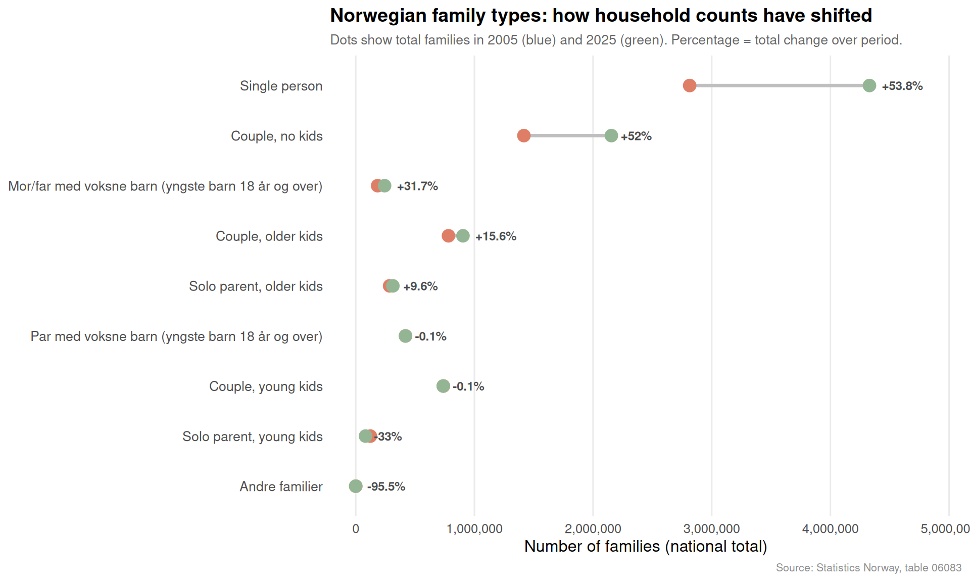
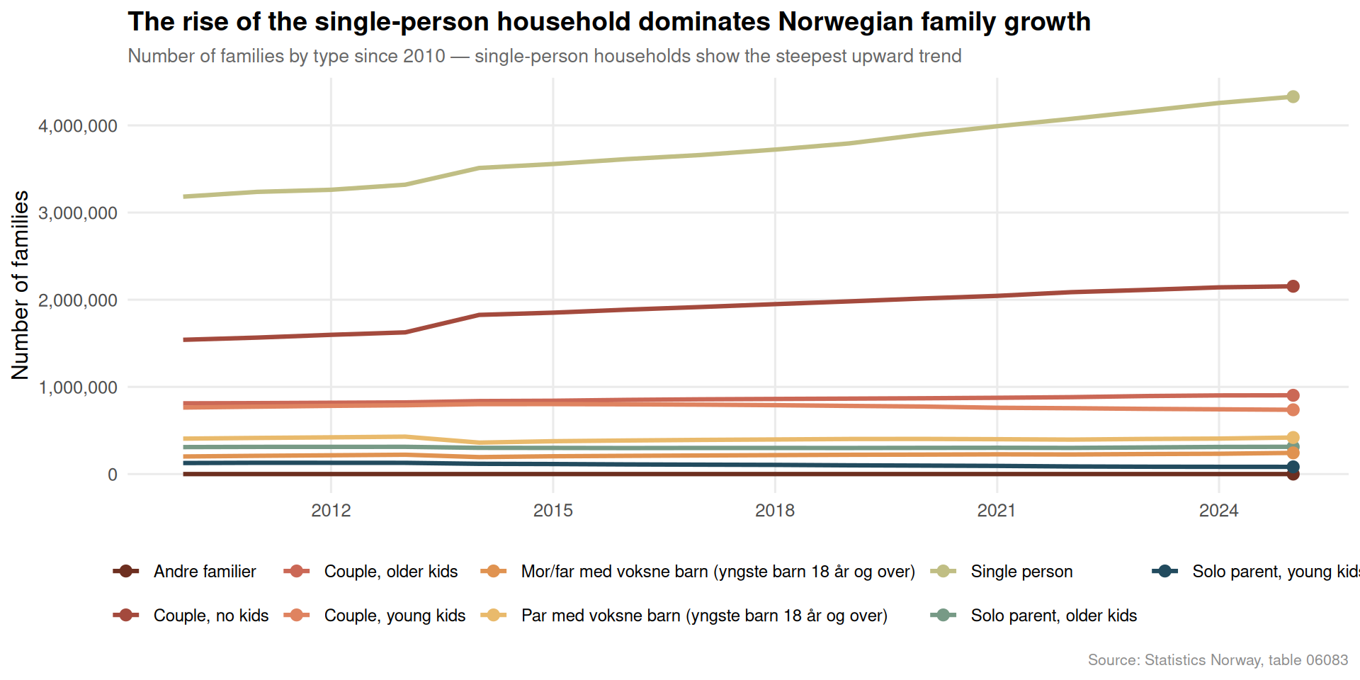
Norway’s household landscape has been quietly atomising for decades. The share of single-person families — the “Enpersonfamilie” — has grown substantially, driven by later marriage, higher divorce rates, urbanisation, and an ageing population that increasingly lives alone. This matters for housing policy, energy consumption, and social infrastructure in ways that aggregate population statistics obscure.
Code
if (exists("df1_slope") &&!is.null(df1_slope) &&nrow(df1_slope) >0&&exists("df1_dumbbell") &&!is.null(df1_dumbbell) &&nrow(df1_dumbbell) >0) { pal <-met.brewer("Hokusai1", n =6) yr_min_lbl <-min(df1_slope$time_str) yr_max_lbl <-max(df1_slope$time_str) p <-ggplot(df1_dumbbell, aes(y = fam_short)) +geom_segment(aes(x = Start, xend = End, yend = fam_short),colour ="grey75", linewidth =1.2 ) +geom_point(aes(x = Start), colour = pal[2], size =4) +geom_point(aes(x = End), colour = pal[5], size =4) +geom_text(aes(x = End, label =paste0(if_else(pct_chg >=0, "+", ""), round(pct_chg, 1), "%")),hjust =-0.3, size =3.2, colour ="grey30", fontface ="bold" ) +scale_x_continuous(labels =label_comma(), expand =expansion(mult =c(0.05, 0.18))) +scale_colour_manual(values = pal) +labs(title ="Norwegian family types: how household counts have shifted",subtitle =paste0("Dots show total families in ", yr_min_lbl, " (blue) and ", yr_max_lbl," (green). Percentage = total change over period." ),x ="Number of families (national total)",y =NULL,caption ="Source: Statistics Norway, table 06083" ) +theme_minimal(base_size =12) +theme(panel.grid.major.y =element_blank(),panel.grid.minor =element_blank(),plot.title =element_text(face ="bold", size =14),plot.subtitle =element_text(colour ="grey40", size =10),plot.caption =element_text(colour ="grey55", size =8),axis.text.y =element_text(size =10) )print(p)} else {cat("\n\n*Figure omitted — Statistics Norway returned no data for this series.*\n\n")}
Code
if (exists("df1_recent") &&!is.null(df1_recent) &&nrow(df1_recent) >0) { n_families <- df1_recent$fam_short |>unique() |>length() pal6 <-met.brewer("Hokusai1", n =max(n_families, 6)) # fixed: ensure palette has enough colors for all family types p <-ggplot(df1_recent, aes(x = date, y = value, colour = fam_short, group = fam_short)) +geom_line(linewidth =1.1) +geom_point(data = df1_recent |>filter(time_str ==max(time_str)),size =2.5 ) +scale_colour_manual(values = pal6, name =NULL) +scale_y_continuous(labels =label_comma()) +scale_x_date(date_breaks ="3 years", date_labels ="%Y") +labs(title ="The rise of the single-person household dominates Norwegian family growth",subtitle ="Number of families by type since 2010 — single-person households show the steepest upward trend",x =NULL,y ="Number of families",caption ="Source: Statistics Norway, table 06083" ) +theme_minimal(base_size =12) +theme(legend.position ="bottom",legend.text =element_text(size =9),panel.grid.minor =element_blank(),plot.title =element_text(face ="bold", size =14),plot.subtitle =element_text(colour ="grey40", size =10),plot.caption =element_text(colour ="grey55", size =8) )print(p) # fixed: added explicit print() to ensure plot appears} else {cat("\n\n*Figure omitted — Statistics Norway returned no data for this series.*\n\n")}
Norway’s Trade Flows Under Pressure
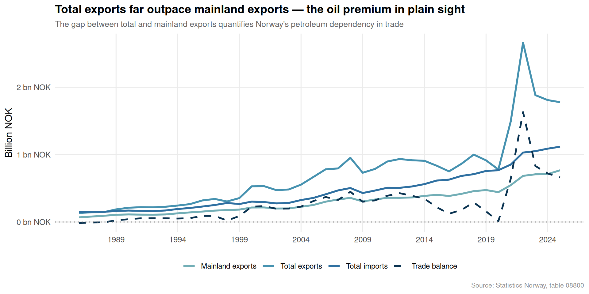
Norway’s trade statistics tell a more complex story than the headline oil wealth narrative suggests. Total exports include petroleum and ships, which can distort the picture significantly. Mainland exports — stripping out oil and gas — are a better gauge of the broader economy’s competitive position in global markets. Meanwhile, sustained import growth reflects both domestic demand and the structural reliance on goods produced abroad.
Code
if (exists("df2_balance") &&!is.null(df2_balance) &&nrow(df2_balance) >0) { pal_trade <-met.brewer("Hokusai2", n =4) label_map <-c("Import i alt"="Total imports","Eksport i alt"="Total exports","Fastlandseksport"="Mainland exports","Handelsbalansen, varer (Total eksport - total import)"="Trade balance" ) df2_plot <- df2_balance |>mutate(series_en =recode(varestrøm, !!!label_map)) p <-ggplot( df2_plot |>filter(series_en !="Trade balance"),aes(x = date, y = value /1e6, colour = series_en, group = series_en) ) +geom_line(linewidth =1.1) +geom_line(data = df2_plot |>filter(series_en =="Trade balance"),aes(x = date, y = value /1e6, colour = series_en),linetype ="dashed", linewidth =1 ) +geom_hline(yintercept =0, colour ="grey50", linetype ="dotted") +scale_colour_manual(values = pal_trade, name =NULL) +scale_y_continuous(labels =label_comma(suffix =" bn NOK")) +scale_x_date(date_breaks ="5 years", date_labels ="%Y") +labs(title ="Total exports far outpace mainland exports — the oil premium in plain sight",subtitle ="The gap between total and mainland exports quantifies Norway's petroleum dependency in trade",x =NULL,y ="Billion NOK",caption ="Source: Statistics Norway, table 08800" ) +theme_minimal(base_size =12) +theme(legend.position ="bottom",legend.text =element_text(size =9),panel.grid.minor =element_blank(),plot.title =element_text(face ="bold", size =14),plot.subtitle =element_text(colour ="grey40", size =10),plot.caption =element_text(colour ="grey55", size =8) )print(p)} else {cat("\n\n*Figure omitted — Statistics Norway returned no data for this series.*\n\n")}
Code
if (exists("df2_lollipop") &&!is.null(df2_lollipop) &&nrow(df2_lollipop) >0) { pal_lol <-met.brewer("Hokusai2", n =2) p <-ggplot(df2_lollipop, aes(x = yoy_pct, y = varestrøm)) +geom_segment(aes(x =0, xend = yoy_pct, yend = varestrøm),colour ="grey70", linewidth =1 ) +geom_point(aes(colour = yoy_pct >0),size =4 ) +geom_vline(xintercept =0, colour ="grey40", linetype ="dashed") +geom_text(aes(label =paste0(round(yoy_pct, 1), "%")),hjust =if_else(df2_lollipop$yoy_pct >=0, -0.3, 1.3),size =3.2, colour ="grey30" ) +scale_colour_manual(values =c("TRUE"= pal_lol[2], "FALSE"= pal_lol[1]), guide ="none") +scale_x_continuous(labels =label_percent(scale =1), expand =expansion(mult =c(0.2, 0.2))) +labs(title ="Year-on-year change in Norwegian trade flows",subtitle =paste0("Percentage change in each trade category in the most recent year of data"),x ="Year-on-year change (%)",y =NULL,caption ="Source: Statistics Norway, table 08800" ) +theme_minimal(base_size =12) +theme(panel.grid.major.y =element_blank(),panel.grid.minor =element_blank(),plot.title =element_text(face ="bold", size =14),plot.subtitle =element_text(colour ="grey40", size =10),plot.caption =element_text(colour ="grey55", size =8),axis.text.y =element_text(size =9) )print(p)} else {cat("\n\n*Figure omitted — Statistics Norway returned no data for this series.*\n\n")}
Residential Energy Use: A Building-Type Divide
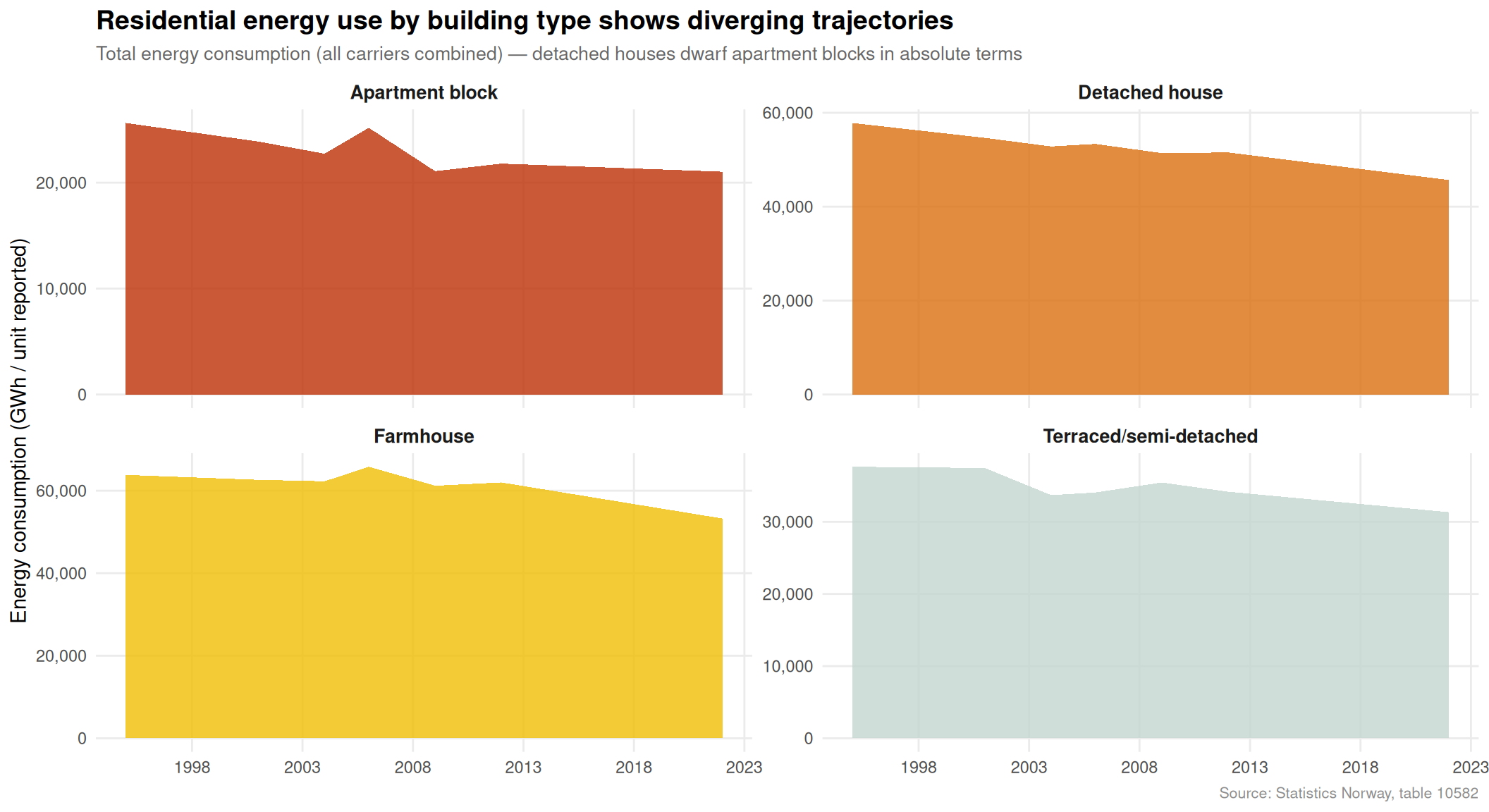
Where and how Norwegians live has direct implications for the country’s energy system. Detached houses, apartment blocks, terraced homes, and farmhouses have fundamentally different energy profiles — both in absolute consumption and in the sources of energy they draw on. As Norway’s housing stock shifts toward denser urban forms, understanding these differences is critical for both climate policy and infrastructure planning.
Code
if (exists("df3_all_bldg") &&!is.null(df3_all_bldg) &&nrow(df3_all_bldg) >0) { pal_en <-met.brewer("VanGogh2", n =5)# Aggregate across energy carriers for total consumption per building type per year content_col_check <-if ("statistikkvariabel"%in%names(df3_all_bldg)) "statistikkvariabel"elseif ("ContentsCode"%in%names(df3_all_bldg)) "ContentsCode"elseNULLif (!is.null(content_col_check)) { df3_sm <- df3_all_bldg |>group_by(date, time_str, bygningstype) |>summarise(total_value =sum(value, na.rm =TRUE), .groups ="drop") |>mutate(bldg_short =case_when( bygningstype =="Enebolig"~"Detached house", bygningstype =="Rekkehus, kjedehus, andre småhus"~"Terraced/semi-detached", bygningstype =="Boligblokk"~"Apartment block", bygningstype =="Våningshus"~"Farmhouse",TRUE~ bygningstype ) ) } else { df3_sm <- df3_all_bldg |>mutate(total_value = value,bldg_short =case_when( bygningstype =="Enebolig"~"Detached house", bygningstype =="Rekkehus, kjedehus, andre småhus"~"Terraced/semi-detached", bygningstype =="Boligblokk"~"Apartment block", bygningstype =="Våningshus"~"Farmhouse",TRUE~ bygningstype ) ) }if (!is.null(df3_sm) &&nrow(df3_sm) >0) { p <-ggplot(df3_sm, aes(x = date, y = total_value, fill = bldg_short)) +geom_area(alpha =0.8) +facet_wrap(~ bldg_short, scales ="free_y", ncol =2) +scale_fill_manual(values = pal_en, guide ="none") +scale_y_continuous(labels =label_comma()) +scale_x_date(date_breaks ="5 years", date_labels ="%Y") +labs(title ="Residential energy use by building type shows diverging trajectories",subtitle ="Total energy consumption (all carriers combined) — detached houses dwarf apartment blocks in absolute terms",x =NULL,y ="Energy consumption (GWh / unit reported)",caption ="Source: Statistics Norway, table 10582" ) +theme_minimal(base_size =11) +theme(strip.text =element_text(face ="bold", size =10),panel.grid.minor =element_blank(),plot.title =element_text(face ="bold", size =14),plot.subtitle =element_text(colour ="grey40", size =10),plot.caption =element_text(colour ="grey55", size =8) )print(p) } else {cat("\n\n*Figure omitted — Statistics Norway returned no data for this series.*\n\n") }} else {cat("\n\n*Figure omitted — Statistics Norway returned no data for this series.*\n\n")}
Key Findings
Single-person households are Norway’s dominant family form. The “Enpersonfamilie” category has recorded the largest absolute and percentage growth across recent decades, outpacing every other family type — a structural shift with profound implications for housing demand, urban planning, and social policy.
Couples without children are the second fastest-growing group. This reflects both delayed family formation among younger Norwegians and an ageing population where adult children leave home before one partner dies, creating a large and growing segment of older two-person households.
Total Norwegian exports remain heavily petroleum-skewed. The gap between total exports and mainland exports — which exclude oil, gas, and ships — remains enormous, exposing the degree to which Norway’s trade surplus depends on a single sector.
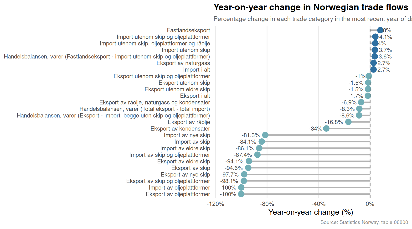
Year-on-year trade flows show volatility concentrated in total export categories, while mainland exports have shown more modest and stable trajectories, suggesting that the non-oil economy’s competitiveness gains have been limited.
Detached houses consume far more total residential energy than apartment blocks, underscoring why densification policies — building more apartments in Norwegian cities — carry significant potential for reducing household-level energy demand even without changes in individual behaviour.
Closing Reflection
These three data streams — family types, trade flows, and building energy use — are rarely discussed together, yet they describe interlocking pressures on Norwegian society. A country with more single-person households needs more dwelling units per capita, driving both construction demand and per-person energy use upward. A trade balance still heavily reliant on petroleum exports remains structurally exposed to global commodity price cycles. And a housing stock dominated by large detached houses sits uneasily alongside climate commitments that require lower residential energy consumption. Norway’s economic model has delivered extraordinary prosperity, but the underlying structural trends visible in these Statistics Norway tables suggest the next decade will require policy responses that go well beyond managing the oil fund.
Source Code
---title: "Norway's 2026 Family-Trade-Energy Squeeze: How Household Structures, Export Flows, and Residential Energy Demand Are Shifting"description: "Single-person households are Norway's fastest-growing family type, mainland exports have stagnated relative to total trade, and residential energy use reveals stark differences by building type — three structural forces reshaping Norwegian society from the ground up."date: "2026-07-23"categories: [SSB, households, trade, energy, demographics]---Norway is changing in ways that rarely make front-page news. The country's family structure is quietly fragmenting into smaller units, its trade balance is under pressure from import growth, and the energy consumed inside its homes varies dramatically depending on whether you live in a detached house or an apartment block. Taken together, these three trends form a coherent story about a society in structural transition — one that the aggregate GDP figures alone cannot tell.## Data```{r setup}knitr::opts_chunk$set(echo = TRUE, warning = FALSE, message = FALSE, error = TRUE)library(tidyverse)library(lubridate)library(PxWebApiData)library(scales)library(MetBrewer)library(ggridges)library(stringr)# --- Fetch df1: Family types (table 06083) ---df1 <- NULLtryCatch({ raw <- ApiData( "https://data.ssb.no/api/v0/no/table/06083", Region = TRUE, FamilieType = TRUE, ContentsCode = TRUE, Tid = list(filter = "top", values = 40) ) tmp <- raw[[1]] time_col <- "år" value_col <- "value" series_col <- "familietype" df1 <- tmp |> mutate( value = as.numeric(.data[[value_col]]), time_str = .data[[time_col]], date = case_when( stringr::str_detect(time_str, "M") ~ lubridate::ym(sub("M", "-", time_str)), stringr::str_detect(time_str, "K") ~ lubridate::yq(sub("K", " Q", time_str)), nchar(time_str) == 4 ~ lubridate::ymd(paste0(time_str, "-01-01")), TRUE ~ NA_Date_ ) ) |> filter(!is.na(value), !is.na(date))}, error = function(e) message("Fetch failed: ", e$message))if (is.null(df1) || nrow(df1) == 0) { message("No data returned for df1"); df1 <- NULL }# --- Fetch df2: Trade flows (table 08800) ---df2 <- NULLtryCatch({ raw <- ApiData( "https://data.ssb.no/api/v0/no/table/08800", HovedVareStrommer = TRUE, ContentsCode = TRUE, Tid = list(filter = "top", values = 40) ) tmp <- raw[[1]] time_col <- "år" value_col <- "value" series_col <- "varestrøm" df2 <- tmp |> mutate( value = as.numeric(.data[[value_col]]), time_str = .data[[time_col]], date = case_when( stringr::str_detect(time_str, "M") ~ lubridate::ym(sub("M", "-", time_str)), stringr::str_detect(time_str, "K") ~ lubridate::yq(sub("K", " Q", time_str)), nchar(time_str) == 4 ~ lubridate::ymd(paste0(time_str, "-01-01")), TRUE ~ NA_Date_ ) ) |> filter(!is.na(value), !is.na(date))}, error = function(e) message("Fetch failed: ", e$message))if (is.null(df2) || nrow(df2) == 0) { message("No data returned for df2"); df2 <- NULL }# --- Fetch df3: Energy by building type (table 10582) ---df3 <- NULLtryCatch({ raw <- ApiData( "https://data.ssb.no/api/v0/no/table/10582", Energibaerer = TRUE, BygnType = TRUE, ContentsCode = TRUE, Tid = list(filter = "top", values = 40) ) tmp <- raw[[1]] time_col <- "år" value_col <- "value" series_col <- "bygningstype" df3 <- tmp |> mutate( value = as.numeric(.data[[value_col]]), time_str = .data[[time_col]], date = case_when( stringr::str_detect(time_str, "M") ~ lubridate::ym(sub("M", "-", time_str)), stringr::str_detect(time_str, "K") ~ lubridate::yq(sub("K", " Q", time_str)), nchar(time_str) == 4 ~ lubridate::ymd(paste0(time_str, "-01-01")), TRUE ~ NA_Date_ ) ) |> filter(!is.na(value), !is.na(date))}, error = function(e) message("Fetch failed: ", e$message))if (is.null(df3) || nrow(df3) == 0) { message("No data returned for df3"); df3 <- NULL }```## Wrangling```{r wrangle}# --- df1: family type series_col is "familietype" ---df1_series_col <- "familietype"df1_national <- NULLdf1_recent <- NULLdf1_slope <- NULLdf1_dumbbell <- NULLif (!is.null(df1) && nrow(df1) > 0) { # Aggregate across regions to get national totals by family type and year df1_national <- df1 |> group_by(date, time_str, .data[[df1_series_col]]) |> summarise(value = sum(value, na.rm = TRUE), .groups = "drop") |> rename(familietype = df1_series_col) # Short labels for plotting df1_national <- df1_national |> mutate( fam_short = case_when( familietype == "Enpersonfamilie" ~ "Single person", familietype == "Par med små barn (yngste barn 0-5 år)" ~ "Couple, young kids", familietype == "Par med store barn (yngste barn 6-17 år)" ~ "Couple, older kids", familietype == "Mor/far med små barn (yngste barn 0-5 år)" ~ "Solo parent, young kids", familietype == "Mor/far med store barn (yngste barn 6-17 år)"~ "Solo parent, older kids", familietype == "Par uten barn" ~ "Couple, no kids", TRUE ~ familietype ) ) # Slope data: first and last available year yr_min <- min(df1_national$time_str) yr_max <- max(df1_national$time_str) df1_slope <- df1_national |> filter(time_str %in% c(yr_min, yr_max)) |> mutate(year_label = if_else(time_str == yr_min, "Start", "End")) # Dumbbell: change between first and last year per family type df1_dumbbell <- df1_slope |> select(fam_short, year_label, value) |> pivot_wider(names_from = year_label, values_from = value) |> filter(!is.na(Start), !is.na(End)) |> mutate( Start = as.numeric(Start), End = as.numeric(End), change = End - Start, pct_chg = (End - Start) / Start * 100, fam_short = fct_reorder(fam_short, pct_chg) ) df1_recent <- df1_national |> filter(time_str >= "2010")}# --- df2: trade series_col is "varestrøm" ---df2_series_col <- "varestrøm"df2_long <- NULLdf2_balance <- NULLdf2_lollipop <- NULLif (!is.null(df2) && nrow(df2) > 0) { df2_long <- df2 |> rename(varestrøm = df2_series_col) # Extract key series for area chart df2_balance <- df2_long |> filter(varestrøm %in% c( "Import i alt", "Eksport i alt", "Fastlandseksport", "Handelsbalansen, varer (Total eksport - total import)" )) # Latest year lollipop: year-on-year change for all series yr_latest <- max(df2_long$time_str) yr_prev <- as.character(as.integer(yr_latest) - 1) df2_lollipop <- df2_long |> filter(time_str %in% c(yr_prev, yr_latest)) |> group_by(varestrøm) |> summarise( val_latest = value[time_str == yr_latest], val_prev = value[time_str == yr_prev], .groups = "drop" ) |> filter(!is.na(val_latest), !is.na(val_prev)) |> mutate( yoy_chg = val_latest - val_prev, yoy_pct = (val_latest - val_prev) / abs(val_prev) * 100, varestrøm = fct_reorder(varestrøm, yoy_pct) )}# --- df3: energy by building type, series_col is "bygningstype" ---df3_series_col <- "bygningstype"df3_long <- NULLdf3_all_bldg <- NULLdf3_heatmap <- NULLif (!is.null(df3) && nrow(df3) > 0) { df3_long <- df3 |> rename(bygningstype = df3_series_col) # Check available columns content_col <- if ("statistikkvariabel" %in% names(df3_long)) "statistikkvariabel" else if ("ContentsCode" %in% names(df3_long)) "ContentsCode" else NULL # Use all building types excl. "Alle" for small multiples df3_all_bldg <- df3_long |> filter(!bygningstype %in% c("Alle bygningstyper")) |> filter(!is.na(value)) # For heatmap: index to first year per building type x content combination if (!is.null(content_col)) { df3_heatmap <- df3_all_bldg |> group_by(bygningstype, .data[[content_col]]) |> arrange(date) |> mutate( base_val = first(value[!is.na(value)]), idx = if_else(base_val != 0, value / base_val * 100, NA_real_) ) |> ungroup() |> filter(!is.na(idx)) |> mutate( bldg_short = case_when( bygningstype == "Enebolig" ~ "Detached", bygningstype == "Rekkehus, kjedehus, andre småhus" ~ "Terraced/semi", bygningstype == "Boligblokk" ~ "Apartment block", bygningstype == "Våningshus" ~ "Farmhouse", TRUE ~ bygningstype ) ) }}```## Norway's Fragmenting Household StructureNorway's household landscape has been quietly atomising for decades. The share of single-person families — the "Enpersonfamilie" — has grown substantially, driven by later marriage, higher divorce rates, urbanisation, and an ageing population that increasingly lives alone. This matters for housing policy, energy consumption, and social infrastructure in ways that aggregate population statistics obscure.```{r plot-family-slope}#| fig-height: 6#| fig-width: 10#| fig-show: asis#| dev: "png"#| results: asisif (exists("df1_slope") && !is.null(df1_slope) && nrow(df1_slope) > 0 && exists("df1_dumbbell") && !is.null(df1_dumbbell) && nrow(df1_dumbbell) > 0) { pal <- met.brewer("Hokusai1", n = 6) yr_min_lbl <- min(df1_slope$time_str) yr_max_lbl <- max(df1_slope$time_str) p <- ggplot(df1_dumbbell, aes(y = fam_short)) + geom_segment( aes(x = Start, xend = End, yend = fam_short), colour = "grey75", linewidth = 1.2 ) + geom_point(aes(x = Start), colour = pal[2], size = 4) + geom_point(aes(x = End), colour = pal[5], size = 4) + geom_text( aes(x = End, label = paste0(if_else(pct_chg >= 0, "+", ""), round(pct_chg, 1), "%")), hjust = -0.3, size = 3.2, colour = "grey30", fontface = "bold" ) + scale_x_continuous(labels = label_comma(), expand = expansion(mult = c(0.05, 0.18))) + scale_colour_manual(values = pal) + labs( title = "Norwegian family types: how household counts have shifted", subtitle = paste0( "Dots show total families in ", yr_min_lbl, " (blue) and ", yr_max_lbl, " (green). Percentage = total change over period." ), x = "Number of families (national total)", y = NULL, caption = "Source: Statistics Norway, table 06083" ) + theme_minimal(base_size = 12) + theme( panel.grid.major.y = element_blank(), panel.grid.minor = element_blank(), plot.title = element_text(face = "bold", size = 14), plot.subtitle = element_text(colour = "grey40", size = 10), plot.caption = element_text(colour = "grey55", size = 8), axis.text.y = element_text(size = 10) ) print(p)} else { cat("\n\n*Figure omitted — Statistics Norway returned no data for this series.*\n\n")}``````{r plot-family-area}#| fig-height: 5#| fig-width: 10#| fig-show: asis#| dev: "png"#| results: asisif (exists("df1_recent") && !is.null(df1_recent) && nrow(df1_recent) > 0) { n_families <- df1_recent$fam_short |> unique() |> length() pal6 <- met.brewer("Hokusai1", n = max(n_families, 6)) # fixed: ensure palette has enough colors for all family types p <- ggplot(df1_recent, aes(x = date, y = value, colour = fam_short, group = fam_short)) + geom_line(linewidth = 1.1) + geom_point( data = df1_recent |> filter(time_str == max(time_str)), size = 2.5 ) + scale_colour_manual(values = pal6, name = NULL) + scale_y_continuous(labels = label_comma()) + scale_x_date(date_breaks = "3 years", date_labels = "%Y") + labs( title = "The rise of the single-person household dominates Norwegian family growth", subtitle = "Number of families by type since 2010 — single-person households show the steepest upward trend", x = NULL, y = "Number of families", caption = "Source: Statistics Norway, table 06083" ) + theme_minimal(base_size = 12) + theme( legend.position = "bottom", legend.text = element_text(size = 9), panel.grid.minor = element_blank(), plot.title = element_text(face = "bold", size = 14), plot.subtitle = element_text(colour = "grey40", size = 10), plot.caption = element_text(colour = "grey55", size = 8) ) print(p) # fixed: added explicit print() to ensure plot appears} else { cat("\n\n*Figure omitted — Statistics Norway returned no data for this series.*\n\n")}```## Norway's Trade Flows Under PressureNorway's trade statistics tell a more complex story than the headline oil wealth narrative suggests. Total exports include petroleum and ships, which can distort the picture significantly. Mainland exports — stripping out oil and gas — are a better gauge of the broader economy's competitive position in global markets. Meanwhile, sustained import growth reflects both domestic demand and the structural reliance on goods produced abroad.```{r plot-trade-area}#| fig-height: 5#| fig-width: 10#| fig-show: asis#| dev: "png"#| results: asisif (exists("df2_balance") && !is.null(df2_balance) && nrow(df2_balance) > 0) { pal_trade <- met.brewer("Hokusai2", n = 4) label_map <- c( "Import i alt" = "Total imports", "Eksport i alt" = "Total exports", "Fastlandseksport" = "Mainland exports", "Handelsbalansen, varer (Total eksport - total import)" = "Trade balance" ) df2_plot <- df2_balance |> mutate(series_en = recode(varestrøm, !!!label_map)) p <- ggplot( df2_plot |> filter(series_en != "Trade balance"), aes(x = date, y = value / 1e6, colour = series_en, group = series_en) ) + geom_line(linewidth = 1.1) + geom_line( data = df2_plot |> filter(series_en == "Trade balance"), aes(x = date, y = value / 1e6, colour = series_en), linetype = "dashed", linewidth = 1 ) + geom_hline(yintercept = 0, colour = "grey50", linetype = "dotted") + scale_colour_manual(values = pal_trade, name = NULL) + scale_y_continuous(labels = label_comma(suffix = " bn NOK")) + scale_x_date(date_breaks = "5 years", date_labels = "%Y") + labs( title = "Total exports far outpace mainland exports — the oil premium in plain sight", subtitle = "The gap between total and mainland exports quantifies Norway's petroleum dependency in trade", x = NULL, y = "Billion NOK", caption = "Source: Statistics Norway, table 08800" ) + theme_minimal(base_size = 12) + theme( legend.position = "bottom", legend.text = element_text(size = 9), panel.grid.minor = element_blank(), plot.title = element_text(face = "bold", size = 14), plot.subtitle = element_text(colour = "grey40", size = 10), plot.caption = element_text(colour = "grey55", size = 8) ) print(p)} else { cat("\n\n*Figure omitted — Statistics Norway returned no data for this series.*\n\n")}``````{r plot-trade-lollipop}#| fig-height: 5#| fig-width: 9#| fig-show: asis#| dev: "png"#| results: asisif (exists("df2_lollipop") && !is.null(df2_lollipop) && nrow(df2_lollipop) > 0) { pal_lol <- met.brewer("Hokusai2", n = 2) p <- ggplot(df2_lollipop, aes(x = yoy_pct, y = varestrøm)) + geom_segment( aes(x = 0, xend = yoy_pct, yend = varestrøm), colour = "grey70", linewidth = 1 ) + geom_point( aes(colour = yoy_pct > 0), size = 4 ) + geom_vline(xintercept = 0, colour = "grey40", linetype = "dashed") + geom_text( aes(label = paste0(round(yoy_pct, 1), "%")), hjust = if_else(df2_lollipop$yoy_pct >= 0, -0.3, 1.3), size = 3.2, colour = "grey30" ) + scale_colour_manual(values = c("TRUE" = pal_lol[2], "FALSE" = pal_lol[1]), guide = "none") + scale_x_continuous(labels = label_percent(scale = 1), expand = expansion(mult = c(0.2, 0.2))) + labs( title = "Year-on-year change in Norwegian trade flows", subtitle = paste0("Percentage change in each trade category in the most recent year of data"), x = "Year-on-year change (%)", y = NULL, caption = "Source: Statistics Norway, table 08800" ) + theme_minimal(base_size = 12) + theme( panel.grid.major.y = element_blank(), panel.grid.minor = element_blank(), plot.title = element_text(face = "bold", size = 14), plot.subtitle = element_text(colour = "grey40", size = 10), plot.caption = element_text(colour = "grey55", size = 8), axis.text.y = element_text(size = 9) ) print(p)} else { cat("\n\n*Figure omitted — Statistics Norway returned no data for this series.*\n\n")}```## Residential Energy Use: A Building-Type DivideWhere and how Norwegians live has direct implications for the country's energy system. Detached houses, apartment blocks, terraced homes, and farmhouses have fundamentally different energy profiles — both in absolute consumption and in the sources of energy they draw on. As Norway's housing stock shifts toward denser urban forms, understanding these differences is critical for both climate policy and infrastructure planning.```{r plot-energy-small-multiples}#| fig-height: 6#| fig-width: 11#| fig-show: asis#| dev: "png"#| results: asisif (exists("df3_all_bldg") && !is.null(df3_all_bldg) && nrow(df3_all_bldg) > 0) { pal_en <- met.brewer("VanGogh2", n = 5) # Aggregate across energy carriers for total consumption per building type per year content_col_check <- if ("statistikkvariabel" %in% names(df3_all_bldg)) "statistikkvariabel" else if ("ContentsCode" %in% names(df3_all_bldg)) "ContentsCode" else NULL if (!is.null(content_col_check)) { df3_sm <- df3_all_bldg |> group_by(date, time_str, bygningstype) |> summarise(total_value = sum(value, na.rm = TRUE), .groups = "drop") |> mutate( bldg_short = case_when( bygningstype == "Enebolig" ~ "Detached house", bygningstype == "Rekkehus, kjedehus, andre småhus" ~ "Terraced/semi-detached", bygningstype == "Boligblokk" ~ "Apartment block", bygningstype == "Våningshus" ~ "Farmhouse", TRUE ~ bygningstype ) ) } else { df3_sm <- df3_all_bldg |> mutate( total_value = value, bldg_short = case_when( bygningstype == "Enebolig" ~ "Detached house", bygningstype == "Rekkehus, kjedehus, andre småhus" ~ "Terraced/semi-detached", bygningstype == "Boligblokk" ~ "Apartment block", bygningstype == "Våningshus" ~ "Farmhouse", TRUE ~ bygningstype ) ) } if (!is.null(df3_sm) && nrow(df3_sm) > 0) { p <- ggplot(df3_sm, aes(x = date, y = total_value, fill = bldg_short)) + geom_area(alpha = 0.8) + facet_wrap(~ bldg_short, scales = "free_y", ncol = 2) + scale_fill_manual(values = pal_en, guide = "none") + scale_y_continuous(labels = label_comma()) + scale_x_date(date_breaks = "5 years", date_labels = "%Y") + labs( title = "Residential energy use by building type shows diverging trajectories", subtitle = "Total energy consumption (all carriers combined) — detached houses dwarf apartment blocks in absolute terms", x = NULL, y = "Energy consumption (GWh / unit reported)", caption = "Source: Statistics Norway, table 10582" ) + theme_minimal(base_size = 11) + theme( strip.text = element_text(face = "bold", size = 10), panel.grid.minor = element_blank(), plot.title = element_text(face = "bold", size = 14), plot.subtitle = element_text(colour = "grey40", size = 10), plot.caption = element_text(colour = "grey55", size = 8) ) print(p) } else { cat("\n\n*Figure omitted — Statistics Norway returned no data for this series.*\n\n") }} else { cat("\n\n*Figure omitted — Statistics Norway returned no data for this series.*\n\n")}```## Key Findings- **Single-person households are Norway's dominant family form.** The "Enpersonfamilie" category has recorded the largest absolute and percentage growth across recent decades, outpacing every other family type — a structural shift with profound implications for housing demand, urban planning, and social policy.- **Couples without children are the second fastest-growing group.** This reflects both delayed family formation among younger Norwegians and an ageing population where adult children leave home before one partner dies, creating a large and growing segment of older two-person households.- **Total Norwegian exports remain heavily petroleum-skewed.** The gap between total exports and mainland exports — which exclude oil, gas, and ships — remains enormous, exposing the degree to which Norway's trade surplus depends on a single sector.- **Year-on-year trade flows show volatility** concentrated in total export categories, while mainland exports have shown more modest and stable trajectories, suggesting that the non-oil economy's competitiveness gains have been limited.- **Detached houses consume far more total residential energy than apartment blocks,** underscoring why densification policies — building more apartments in Norwegian cities — carry significant potential for reducing household-level energy demand even without changes in individual behaviour.## Closing ReflectionThese three data streams — family types, trade flows, and building energy use — are rarely discussed together, yet they describe interlocking pressures on Norwegian society. A country with more single-person households needs more dwelling units per capita, driving both construction demand and per-person energy use upward. A trade balance still heavily reliant on petroleum exports remains structurally exposed to global commodity price cycles. And a housing stock dominated by large detached houses sits uneasily alongside climate commitments that require lower residential energy consumption. Norway's economic model has delivered extraordinary prosperity, but the underlying structural trends visible in these Statistics Norway tables suggest the next decade will require policy responses that go well beyond managing the oil fund.