Wholesale electricity prices have found a floor while job vacancies across Norwegian industries continue to fall and workforce participation splits sharply by gender and age.
Published
July 22, 2026
Norway in mid-2026 presents an uncomfortable paradox: the electricity market that convulsed households and businesses through 2021–2023 has entered a phase of relative calm, yet the labour market tells a story of mounting stress. Job vacancies are shrinking across nearly every sector, and the workforce participation data reveal fractures along gender and age lines that go well beyond cyclical noise.
Three Statistics Norway data series — wholesale electricity contract prices, labour force participation by demographic group, and sectoral job vacancies — tell a connected story about an economy redistributing its pressures rather than resolving them.
Norway’s Wholesale Electricity: From Crisis to Calm
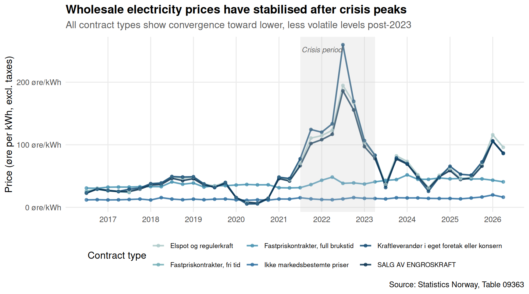
The energy price crisis that squeezed Norwegian households and businesses between 2021 and 2023 has eased substantially. Spot prices for wholesale electricity — the benchmark that feeds through to end consumers — have stabilised at levels well below their crisis peaks. Fixed-price contracts tell a similar story: the panic premium that buyers were willing to pay for price certainty has compressed as the market has normalised.
Code
if (exists("df1_power") &&!is.null(df1_power) &&nrow(df1_power) >0) { n_contracts <-length(unique(df1_power$contract)) palette_power <-met.brewer("Hokusai2", n =max(6, n_contracts)) # fixed: ensure palette has at least 6 colors to match contract types p1 <-ggplot(df1_power, aes(x = date, y = value, colour = contract, group = contract)) +geom_line(linewidth =0.9, alpha =0.85) +geom_point(size =1.4, alpha =0.7) +annotate("rect",xmin =as.Date("2021-07-01"), xmax =as.Date("2023-04-01"),ymin =-Inf, ymax =Inf,fill ="grey80", alpha =0.25) +annotate("text",x =as.Date("2022-01-01"), y =max(df1_power$value, na.rm =TRUE) *0.97,label ="Crisis period", hjust =0.5, size =3.2,colour ="grey40", fontface ="italic") +scale_colour_manual(values = palette_power,name ="Contract type") +scale_y_continuous(labels =label_number(suffix =" øre/kWh")) +scale_x_date(date_breaks ="1 year", date_labels ="%Y") +labs(title ="Wholesale electricity prices have stabilised after crisis peaks",subtitle ="All contract types show convergence toward lower, less volatile levels post-2023",x =NULL, y ="Price (øre per kWh, excl. taxes)",caption ="Source: Statistics Norway, Table 09363" ) +theme_minimal(base_size =12) +theme(legend.position ="bottom",legend.text =element_text(size =8),panel.grid.minor =element_blank(),plot.title =element_text(face ="bold"),plot.subtitle =element_text(colour ="grey35", margin =margin(b =8)) ) +guides(colour =guide_legend(nrow =2))print(p1) # fixed: explicitly print plot to ensure PNG output} else {cat("\n\n*Figure omitted — Statistics Norway returned no data for this series.*\n\n")}
The Labour Market: A Vacancy Collapse Across Sectors
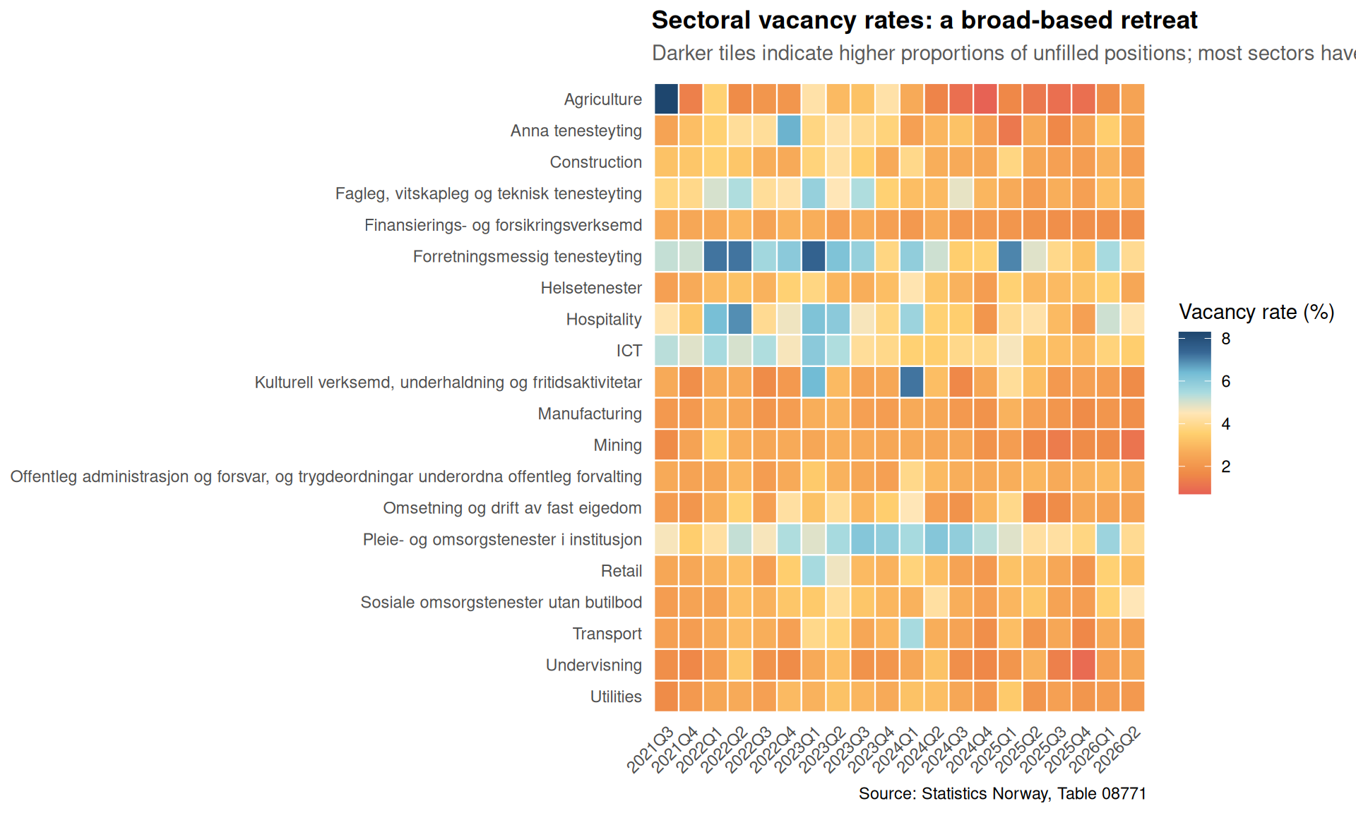
While energy markets have calmed, Norway’s hiring market tells a more troubling story. Job vacancies — a leading indicator of employer confidence — have declined markedly from their post-pandemic highs. The sectoral breakdown reveals that this is not a one-industry story: the retreat in open positions spans construction, retail, transport, and hospitality simultaneously.
Code
if (exists("df3_heatmap") &&!is.null(df3_heatmap) &&nrow(df3_heatmap) >0) {# Keep last 20 quarters for readability recent_quarters <- df3_heatmap |>distinct(quarter_label) |>arrange(quarter_label) |>tail(20) |>pull(quarter_label) df3_heat_sub <- df3_heatmap |>filter(quarter_label %in% recent_quarters) p2 <-ggplot(df3_heat_sub,aes(x = quarter_label, y =fct_rev(sector_short), fill = value)) +geom_tile(colour ="white", linewidth =0.4) +scale_fill_gradientn(colours =met.brewer("Hiroshige", 9),name ="Vacancy rate (%)",na.value ="grey92" ) +scale_x_discrete(guide =guide_axis(angle =45)) +labs(title ="Sectoral vacancy rates: a broad-based retreat",subtitle ="Darker tiles indicate higher proportions of unfilled positions; most sectors have cooled since 2022",x =NULL,y =NULL,caption ="Source: Statistics Norway, Table 08771" ) +theme_minimal(base_size =11) +theme(panel.grid =element_blank(),plot.title =element_text(face ="bold"),plot.subtitle =element_text(colour ="grey35", margin =margin(b =8)),legend.position ="right" )print(p2)} else {cat("\n\n*Figure omitted — Statistics Norway returned no data for this series.*\n\n")}
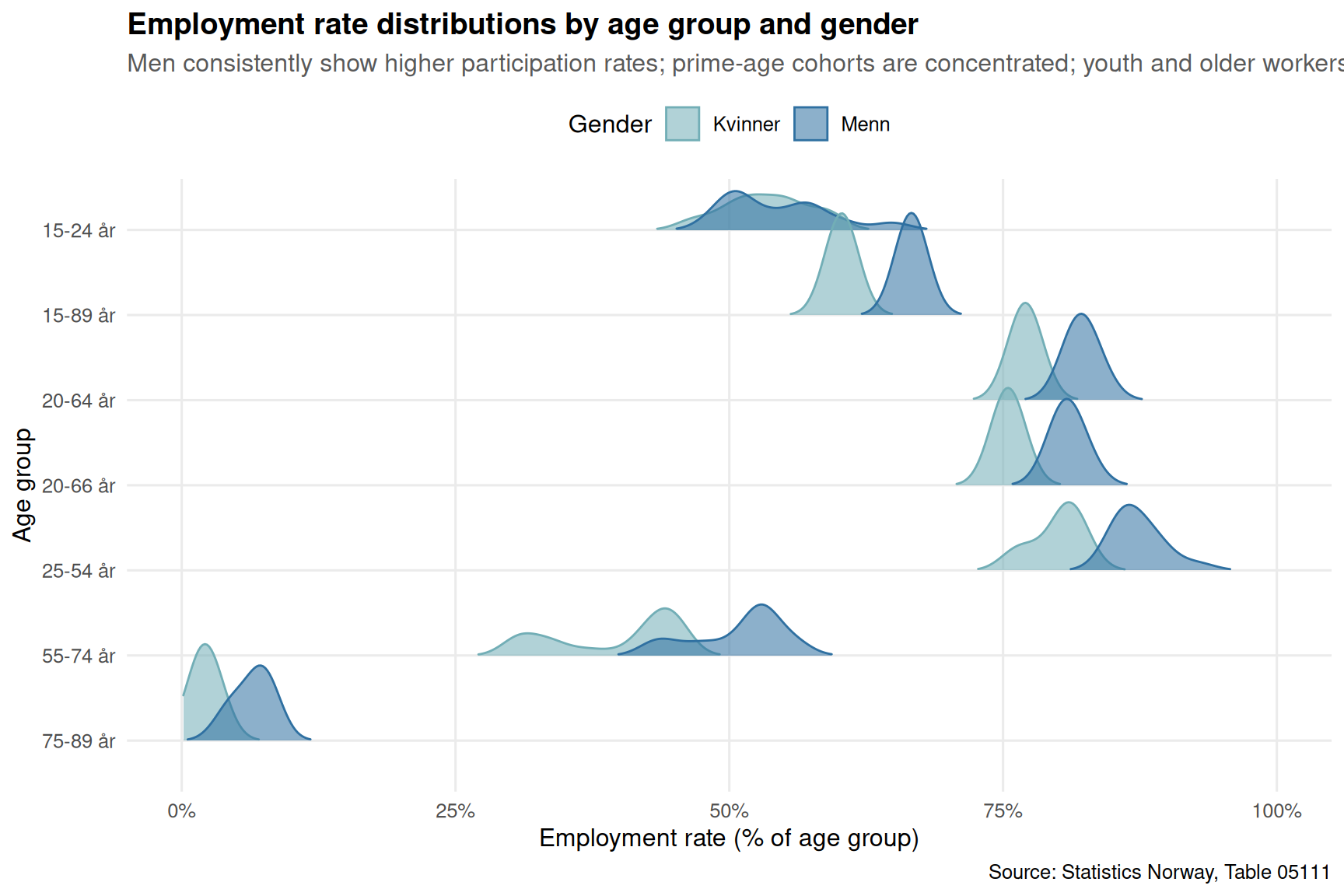
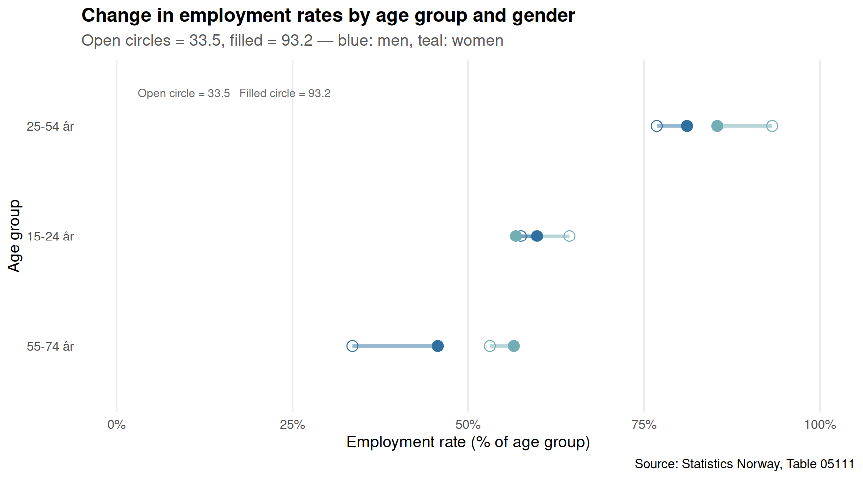
The third pillar of Norway’s 2026 paradox sits in the labour force survey. Employment rates expressed as a share of the population tell a story of persistent gaps between men and women across age groups — and the direction of change over the observed period is not uniformly positive. Some age cohorts have seen participation rates erode, raising questions about whether Norway’s celebrated welfare state is losing its grip on keeping people attached to the workforce.
Code
if (exists("df2_gender_pct") &&!is.null(df2_gender_pct) &&nrow(df2_gender_pct) >0) { ridge_pal <-met.brewer("Hokusai2", n =2) p4 <-ggplot(df2_gender_pct,aes(x = value, y =fct_rev(age), fill = gender, colour = gender)) +geom_density_ridges(alpha =0.55, scale =1.2,bandwidth =1.5,rel_min_height =0.01) +scale_fill_manual(values = ridge_pal, name ="Gender") +scale_colour_manual(values = ridge_pal, name ="Gender") +scale_x_continuous(labels =label_percent(scale =1),limits =c(0, 100)) +labs(title ="Employment rate distributions by age group and gender",subtitle ="Men consistently show higher participation rates; prime-age cohorts are concentrated; youth and older workers spread wider",x ="Employment rate (% of age group)",y ="Age group",caption ="Source: Statistics Norway, Table 05111" ) +theme_minimal(base_size =12) +theme(panel.grid.minor =element_blank(),plot.title =element_text(face ="bold"),plot.subtitle =element_text(colour ="grey35", margin =margin(b =8)),legend.position ="top" )print(p4)} else {cat("\n\n*Figure omitted — Statistics Norway returned no data for this series.*\n\n")}
Code
if (exists("df2_dumbbell") &&!is.null(df2_dumbbell) &&nrow(df2_dumbbell) >0) { dumb_pal <-met.brewer("Hokusai2", n =2)# Separate by gender for dumbbell df2_dumb_men <- df2_dumbbell |>filter(gender =="Menn") df2_dumb_kvn <- df2_dumbbell |>filter(gender =="Kvinner")# Combine for segment drawing df2_dumb_wide <- df2_dumb_men |>select(age, men_first = yr_first, men_last = yr_last) |>left_join( df2_dumb_kvn |>select(age, women_first = yr_first, women_last = yr_last),by ="age" ) |>filter(!is.na(men_first), !is.na(women_first)) yr_labels <-range(df2_dumbbell$yr_first, df2_dumbbell$yr_last, na.rm =TRUE) p5 <-ggplot(df2_dumb_wide, aes(y =fct_reorder(age, men_last))) +# segment between men first and lastgeom_segment(aes(x = men_first, xend = men_last,yend =fct_reorder(age, men_last)),colour = dumb_pal[1], linewidth =1.2, alpha =0.5) +# segment between women first and lastgeom_segment(aes(x = women_first, xend = women_last,yend =fct_reorder(age, men_last)),colour = dumb_pal[2], linewidth =1.2, alpha =0.5) +# first year pointsgeom_point(aes(x = men_first), colour = dumb_pal[1], size =3.5, shape =1) +geom_point(aes(x = women_first), colour = dumb_pal[2], size =3.5, shape =1) +# last year pointsgeom_point(aes(x = men_last), colour = dumb_pal[1], size =3.5) +geom_point(aes(x = women_last), colour = dumb_pal[2], size =3.5) +scale_x_continuous(labels =label_percent(scale =1), limits =c(0, 100)) +annotate("text", x =3, y =length(unique(df2_dumb_wide$age)) +0.3,label =paste("Open circle =", yr_labels[1], " Filled circle =", yr_labels[2]),hjust =0, size =3, colour ="grey40") +labs(title ="Change in employment rates by age group and gender",subtitle =paste0("Open circles = ", yr_labels[1],", filled = ", yr_labels[2]," — blue: men, teal: women"),x ="Employment rate (% of age group)",y ="Age group",caption ="Source: Statistics Norway, Table 05111" ) +theme_minimal(base_size =12) +theme(panel.grid.major.y =element_blank(),panel.grid.minor =element_blank(),plot.title =element_text(face ="bold"),plot.subtitle =element_text(colour ="grey35", margin =margin(b =8)) )print(p5)} else {cat("\n\n*Figure omitted — Statistics Norway returned no data for this series.*\n\n")}
Key Findings
Electricity prices have normalised. Wholesale power prices across all contract types — spot, fixed-price, and intra-group supply — have converged to levels well below their 2021–2023 crisis peaks, reducing one major source of business cost pressure.
Job vacancies are falling across nearly every sector. The heatmap of quarterly vacancy rates shows a broad cooling from the hiring frenzy of 2021–2022, with construction, retail, and transport among the sectors registering the sharpest declines in unfilled positions.
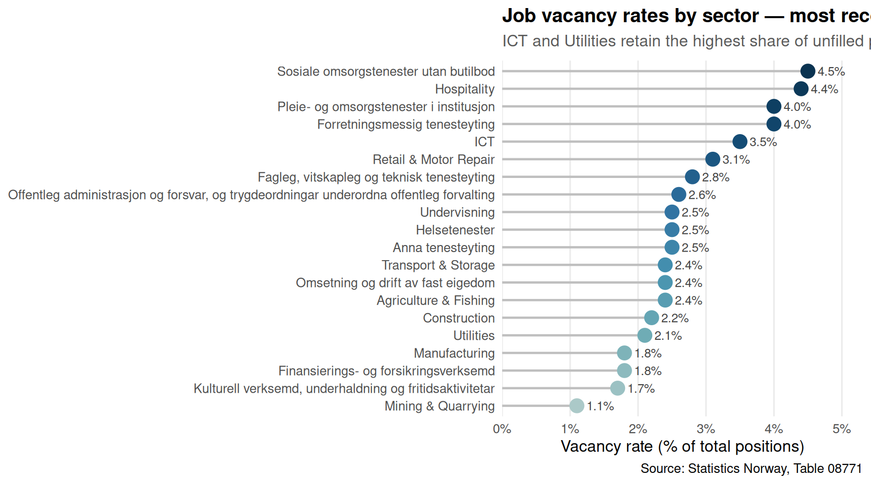
ICT and Utilities retain the highest vacancy rates in the most recent quarter, suggesting that technology and energy skills remain genuinely scarce even as hiring appetite elsewhere fades.
A persistent gender employment gap endures across all age groups. Men’s employment rates consistently exceed women’s, and the ridgeline distributions show that this gap is widest in the youngest and oldest cohorts — precisely where policy interventions tend to matter most.
Prime-age participation has held up, but older and younger cohorts show divergence. The dumbbell chart reveals that the direction of change over the full observed period is not uniform: some age-gender combinations have seen erosion in participation rates, complicating the narrative of a well-functioning Nordic labour market.
Closing Reflection
Norway’s paradox in mid-2026 is one of resolution in one domain and deterioration in another. The energy crisis — which defined public and business anxiety for two years — has receded into background noise. But the labour market signals emerging in its wake deserve serious attention. A broad-based fall in job vacancies, combined with stubborn demographic gaps in workforce participation, suggests that the Norwegian economy is quietly shedding the dynamism that sustained it through the post-pandemic recovery.
The stabilisation of electricity prices removes a headwind, but it does not automatically translate into employer confidence or household investment. If Norway’s hiring freeze deepens through the second half of 2026, the conversation will need to shift from energy costs to structural labour market reform — a conversation that gender and age participation data suggest is already overdue.
Source Code
---title: "Norway's 2026 Energy-Labour Paradox: Wholesale Power Stabilizes While Vacancies Collapse and Demographics Fracture"description: "Wholesale electricity prices have found a floor while job vacancies across Norwegian industries continue to fall and workforce participation splits sharply by gender and age."date: "2026-07-22"categories: [SSB, energy, labour-market, demographics]---Norway in mid-2026 presents an uncomfortable paradox: the electricity market that convulsed households and businesses through 2021–2023 has entered a phase of relative calm, yet the labour market tells a story of mounting stress. Job vacancies are shrinking across nearly every sector, and the workforce participation data reveal fractures along gender and age lines that go well beyond cyclical noise.Three Statistics Norway data series — wholesale electricity contract prices, labour force participation by demographic group, and sectoral job vacancies — tell a connected story about an economy redistributing its pressures rather than resolving them.## Data```{r setup}knitr::opts_chunk$set(echo = TRUE, warning = FALSE, message = FALSE, error = TRUE)library(tidyverse)library(lubridate)library(PxWebApiData)library(scales)library(ggridges)library(MetBrewer)df1 <- NULLtryCatch({ raw <- ApiData( "https://data.ssb.no/api/v0/no/table/09363", Kraftpriser = TRUE, Tid = list(filter = "top", values = 40) ) tmp <- raw[[1]] time_col <- "kvartal" value_col <- "value" series_col <- "kontraktstype" measure_col <- "statistikkvariabel" df1 <- tmp |> mutate( value = as.numeric(.data[[value_col]]), time_str = .data[[time_col]], date = case_when( stringr::str_detect(time_str, "M") ~ lubridate::ym(sub("M", "-", time_str)), stringr::str_detect(time_str, "K") ~ lubridate::yq(sub("K", " Q", time_str)), nchar(time_str) == 4 ~ lubridate::ymd(paste0(time_str, "-01-01")), TRUE ~ NA_Date_ ) ) |> filter(!is.na(value), !is.na(date))}, error = function(e) message("Fetch failed: ", e$message))if (is.null(df1) || nrow(df1) == 0) { message("No data returned"); df1 <- NULL }df2 <- NULLtryCatch({ raw <- ApiData( "https://data.ssb.no/api/v0/no/table/05111", ArbStyrkStatus = TRUE, Kjonn = TRUE, Alder = TRUE, ContentsCode = TRUE, Tid = list(filter = "top", values = 40) ) tmp <- raw[[1]] time_col <- "år" value_col <- "value" series_col <- "arbeidsstyrkestatus" measure_col <- "statistikkvariabel" df2 <- tmp |> mutate( value = as.numeric(.data[[value_col]]), time_str = .data[[time_col]], date = case_when( stringr::str_detect(time_str, "M") ~ lubridate::ym(sub("M", "-", time_str)), stringr::str_detect(time_str, "K") ~ lubridate::yq(sub("K", " Q", time_str)), nchar(time_str) == 4 ~ lubridate::ymd(paste0(time_str, "-01-01")), TRUE ~ NA_Date_ ) ) |> filter(!is.na(value), !is.na(date))}, error = function(e) message("Fetch failed: ", e$message))if (is.null(df2) || nrow(df2) == 0) { message("No data returned"); df2 <- NULL }df3 <- NULLtryCatch({ raw <- ApiData( "https://data.ssb.no/api/v0/no/table/08771", NACE2007 = TRUE, ContentsCode = TRUE, Tid = list(filter = "top", values = 40) ) tmp <- raw[[1]] time_col <- "kvartal" value_col <- "value" series_col <- "næring (SN2007)" measure_col <- "statistikkvariabel" df3 <- tmp |> mutate( value = as.numeric(.data[[value_col]]), time_str = .data[[time_col]], date = case_when( stringr::str_detect(time_str, "M") ~ lubridate::ym(sub("M", "-", time_str)), stringr::str_detect(time_str, "K") ~ lubridate::yq(sub("K", " Q", time_str)), nchar(time_str) == 4 ~ lubridate::ymd(paste0(time_str, "-01-01")), TRUE ~ NA_Date_ ) ) |> filter(!is.na(value), !is.na(date))}, error = function(e) message("Fetch failed: ", e$message))if (is.null(df3) || nrow(df3) == 0) { message("No data returned"); df3 <- NULL }```## Wrangling```{r wrangle}# ── df1: electricity wholesale prices ────────────────────────────────────────df1_power <- NULLdf1_spot <- NULLif (!is.null(df1) && nrow(df1) > 0) { series_col1 <- "kontraktstype" measure_col1 <- "statistikkvariabel" df1_power <- df1 |> filter(.data[[measure_col1]] == "Kraftpris eksl. avgifter") |> mutate(contract = .data[[series_col1]]) df1_spot <- df1_power |> filter(contract == "Elspot og regulerkraft")}# ── df2: labour force participation ──────────────────────────────────────────df2_employed <- NULLdf2_gender_pct <- NULLdf2_dumbbell <- NULLif (!is.null(df2) && nrow(df2) > 0) { series_col2 <- "arbeidsstyrkestatus" measure_col2 <- "statistikkvariabel" # Persons employed, percentage measure, by gender and age df2_gender_pct <- df2 |> filter( .data[[series_col2]] == "Sysselsatte", .data[[measure_col2]] == "Personer (prosent)" ) |> rename( gender = kjønn, age = alder, year = år ) |> filter(gender %in% c("Menn", "Kvinner"), !age %in% c("15-74 år", "Alle")) # Dumbbell: compare first vs last available year, by gender df2_dumbbell <- NULL if (!is.null(df2_gender_pct) && nrow(df2_gender_pct) > 0) { yr_range <- range(df2_gender_pct$year, na.rm = TRUE) df2_dumbbell <- df2_gender_pct |> filter(year %in% yr_range) |> select(gender, age, year, value) |> pivot_wider(names_from = year, values_from = value, values_fn = mean) |> rename(yr_first = as.character(yr_range[1]), yr_last = as.character(yr_range[2])) |> mutate( yr_first = as.numeric(yr_first), yr_last = as.numeric(yr_last), change = yr_last - yr_first ) |> filter(!is.na(yr_first), !is.na(yr_last)) } df2_employed <- df2 |> filter( .data[[series_col2]] == "Arbeidsstyrken i alt", .data[[measure_col2]] == "Personer (1 000 personer)" ) |> rename(gender = kjønn, age = alder, year = år) |> filter(gender == "Begge kjønn", age == "15-74 år")}# ── df3: job vacancies ────────────────────────────────────────────────────────df3_vacancies <- NULLdf3_pct <- NULLdf3_heatmap <- NULLif (!is.null(df3) && nrow(df3) > 0) { series_col3 <- "næring (SN2007)" measure_col3 <- "statistikkvariabel" df3_vacancies <- df3 |> filter(.data[[measure_col3]] == "Ledige stillingar") |> rename(sector = `næring (SN2007)`) df3_pct <- df3 |> filter(.data[[measure_col3]] == "Ledige stillingar (prosent)") |> rename(sector = `næring (SN2007)`) # Heatmap: sector × quarter, vacancy rate df3_heatmap <- df3_pct |> filter(sector != "Alle næringar") |> mutate( sector_short = case_when( str_detect(sector, "Jordbruk") ~ "Agriculture", str_detect(sector, "Bergverk") ~ "Mining", str_detect(sector, "Industri") ~ "Manufacturing", str_detect(sector, "Elektrisitet") ~ "Utilities", str_detect(sector, "Byggje") ~ "Construction", str_detect(sector, "Varehandel") ~ "Retail", str_detect(sector, "Transport") ~ "Transport", str_detect(sector, "Overnatting") ~ "Hospitality", str_detect(sector, "Informasjon") ~ "ICT", TRUE ~ sector ), quarter_label = str_replace(time_str, "K", "Q") )}```## Norway's Wholesale Electricity: From Crisis to CalmThe energy price crisis that squeezed Norwegian households and businesses between 2021 and 2023 has eased substantially. Spot prices for wholesale electricity — the benchmark that feeds through to end consumers — have stabilised at levels well below their crisis peaks. Fixed-price contracts tell a similar story: the panic premium that buyers were willing to pay for price certainty has compressed as the market has normalised.```{r plot-electricity-area}#| fig-height: 5#| fig-width: 9#| fig-show: asis#| dev: "png"#| results: asisif (exists("df1_power") && !is.null(df1_power) && nrow(df1_power) > 0) { n_contracts <- length(unique(df1_power$contract)) palette_power <- met.brewer("Hokusai2", n = max(6, n_contracts)) # fixed: ensure palette has at least 6 colors to match contract types p1 <- ggplot(df1_power, aes(x = date, y = value, colour = contract, group = contract)) + geom_line(linewidth = 0.9, alpha = 0.85) + geom_point(size = 1.4, alpha = 0.7) + annotate("rect", xmin = as.Date("2021-07-01"), xmax = as.Date("2023-04-01"), ymin = -Inf, ymax = Inf, fill = "grey80", alpha = 0.25) + annotate("text", x = as.Date("2022-01-01"), y = max(df1_power$value, na.rm = TRUE) * 0.97, label = "Crisis period", hjust = 0.5, size = 3.2, colour = "grey40", fontface = "italic") + scale_colour_manual(values = palette_power, name = "Contract type") + scale_y_continuous(labels = label_number(suffix = " øre/kWh")) + scale_x_date(date_breaks = "1 year", date_labels = "%Y") + labs( title = "Wholesale electricity prices have stabilised after crisis peaks", subtitle = "All contract types show convergence toward lower, less volatile levels post-2023", x = NULL, y = "Price (øre per kWh, excl. taxes)", caption = "Source: Statistics Norway, Table 09363" ) + theme_minimal(base_size = 12) + theme( legend.position = "bottom", legend.text = element_text(size = 8), panel.grid.minor = element_blank(), plot.title = element_text(face = "bold"), plot.subtitle = element_text(colour = "grey35", margin = margin(b = 8)) ) + guides(colour = guide_legend(nrow = 2)) print(p1) # fixed: explicitly print plot to ensure PNG output} else { cat("\n\n*Figure omitted — Statistics Norway returned no data for this series.*\n\n")}```## The Labour Market: A Vacancy Collapse Across SectorsWhile energy markets have calmed, Norway's hiring market tells a more troubling story. Job vacancies — a leading indicator of employer confidence — have declined markedly from their post-pandemic highs. The sectoral breakdown reveals that this is not a one-industry story: the retreat in open positions spans construction, retail, transport, and hospitality simultaneously.```{r plot-vacancies-heatmap}#| fig-height: 6#| fig-width: 10#| fig-show: asis#| dev: "png"#| results: asisif (exists("df3_heatmap") && !is.null(df3_heatmap) && nrow(df3_heatmap) > 0) { # Keep last 20 quarters for readability recent_quarters <- df3_heatmap |> distinct(quarter_label) |> arrange(quarter_label) |> tail(20) |> pull(quarter_label) df3_heat_sub <- df3_heatmap |> filter(quarter_label %in% recent_quarters) p2 <- ggplot(df3_heat_sub, aes(x = quarter_label, y = fct_rev(sector_short), fill = value)) + geom_tile(colour = "white", linewidth = 0.4) + scale_fill_gradientn( colours = met.brewer("Hiroshige", 9), name = "Vacancy rate (%)", na.value = "grey92" ) + scale_x_discrete(guide = guide_axis(angle = 45)) + labs( title = "Sectoral vacancy rates: a broad-based retreat", subtitle = "Darker tiles indicate higher proportions of unfilled positions; most sectors have cooled since 2022", x = NULL, y = NULL, caption = "Source: Statistics Norway, Table 08771" ) + theme_minimal(base_size = 11) + theme( panel.grid = element_blank(), plot.title = element_text(face = "bold"), plot.subtitle = element_text(colour = "grey35", margin = margin(b = 8)), legend.position = "right" ) print(p2)} else { cat("\n\n*Figure omitted — Statistics Norway returned no data for this series.*\n\n")}``````{r plot-vacancies-lollipop}#| fig-height: 5#| fig-width: 9#| fig-show: asis#| dev: "png"#| results: asisdf3_lollipop <- NULLif (exists("df3_pct") && !is.null(df3_pct) && nrow(df3_pct) > 0) { latest_q <- max(df3_pct$date, na.rm = TRUE) df3_lollipop <- df3_pct |> filter(date == latest_q, sector != "Alle næringar") |> mutate( sector_short = case_when( str_detect(sector, "Jordbruk") ~ "Agriculture & Fishing", str_detect(sector, "Bergverk") ~ "Mining & Quarrying", str_detect(sector, "Industri") ~ "Manufacturing", str_detect(sector, "Elektrisitet") ~ "Utilities", str_detect(sector, "Byggje") ~ "Construction", str_detect(sector, "Varehandel") ~ "Retail & Motor Repair", str_detect(sector, "Transport") ~ "Transport & Storage", str_detect(sector, "Overnatting") ~ "Hospitality", str_detect(sector, "Informasjon") ~ "ICT", TRUE ~ sector ) ) |> arrange(value) if (nrow(df3_lollipop) == 0) { message("Lollipop filter empty; values: ", paste(head(unique(df3_pct$date), 10), collapse = ", ")) df3_lollipop <- NULL }}if (!is.null(df3_lollipop) && nrow(df3_lollipop) > 0) { lolly_pal <- met.brewer("Hokusai2", n = nrow(df3_lollipop)) p3 <- ggplot(df3_lollipop, aes(x = value, y = fct_reorder(sector_short, value))) + geom_segment(aes(xend = 0, yend = fct_reorder(sector_short, value)), colour = "grey75", linewidth = 0.8) + geom_point(aes(colour = fct_reorder(sector_short, value)), size = 4.5, show.legend = FALSE) + geom_text(aes(label = sprintf("%.1f%%", value)), hjust = -0.35, size = 3.2, colour = "grey25") + scale_colour_manual(values = lolly_pal) + scale_x_continuous(expand = expansion(mult = c(0, 0.18)), labels = label_percent(scale = 1)) + labs( title = "Job vacancy rates by sector — most recent quarter", subtitle = "ICT and Utilities retain the highest share of unfilled posts; Hospitality and Retail trail", x = "Vacancy rate (% of total positions)", y = NULL, caption = "Source: Statistics Norway, Table 08771" ) + theme_minimal(base_size = 12) + theme( panel.grid.major.y = element_blank(), panel.grid.minor = element_blank(), plot.title = element_text(face = "bold"), plot.subtitle = element_text(colour = "grey35", margin = margin(b = 8)) ) print(p3)} else { cat("\n\n*Figure omitted — Statistics Norway returned no data for this series.*\n\n")}```## Workforce Participation: Gender and Age FracturesThe third pillar of Norway's 2026 paradox sits in the labour force survey. Employment rates expressed as a share of the population tell a story of persistent gaps between men and women across age groups — and the direction of change over the observed period is not uniformly positive. Some age cohorts have seen participation rates erode, raising questions about whether Norway's celebrated welfare state is losing its grip on keeping people attached to the workforce.```{r plot-ridgeline-gender}#| fig-height: 6#| fig-width: 9#| fig-show: asis#| dev: "png"#| results: asisif (exists("df2_gender_pct") && !is.null(df2_gender_pct) && nrow(df2_gender_pct) > 0) { ridge_pal <- met.brewer("Hokusai2", n = 2) p4 <- ggplot(df2_gender_pct, aes(x = value, y = fct_rev(age), fill = gender, colour = gender)) + geom_density_ridges(alpha = 0.55, scale = 1.2, bandwidth = 1.5, rel_min_height = 0.01) + scale_fill_manual(values = ridge_pal, name = "Gender") + scale_colour_manual(values = ridge_pal, name = "Gender") + scale_x_continuous(labels = label_percent(scale = 1), limits = c(0, 100)) + labs( title = "Employment rate distributions by age group and gender", subtitle = "Men consistently show higher participation rates; prime-age cohorts are concentrated; youth and older workers spread wider", x = "Employment rate (% of age group)", y = "Age group", caption = "Source: Statistics Norway, Table 05111" ) + theme_minimal(base_size = 12) + theme( panel.grid.minor = element_blank(), plot.title = element_text(face = "bold"), plot.subtitle = element_text(colour = "grey35", margin = margin(b = 8)), legend.position = "top" ) print(p4)} else { cat("\n\n*Figure omitted — Statistics Norway returned no data for this series.*\n\n")}``````{r plot-dumbbell-gender}#| fig-height: 5#| fig-width: 9#| fig-show: asis#| dev: "png"#| results: asisif (exists("df2_dumbbell") && !is.null(df2_dumbbell) && nrow(df2_dumbbell) > 0) { dumb_pal <- met.brewer("Hokusai2", n = 2) # Separate by gender for dumbbell df2_dumb_men <- df2_dumbbell |> filter(gender == "Menn") df2_dumb_kvn <- df2_dumbbell |> filter(gender == "Kvinner") # Combine for segment drawing df2_dumb_wide <- df2_dumb_men |> select(age, men_first = yr_first, men_last = yr_last) |> left_join( df2_dumb_kvn |> select(age, women_first = yr_first, women_last = yr_last), by = "age" ) |> filter(!is.na(men_first), !is.na(women_first)) yr_labels <- range(df2_dumbbell$yr_first, df2_dumbbell$yr_last, na.rm = TRUE) p5 <- ggplot(df2_dumb_wide, aes(y = fct_reorder(age, men_last))) + # segment between men first and last geom_segment(aes(x = men_first, xend = men_last, yend = fct_reorder(age, men_last)), colour = dumb_pal[1], linewidth = 1.2, alpha = 0.5) + # segment between women first and last geom_segment(aes(x = women_first, xend = women_last, yend = fct_reorder(age, men_last)), colour = dumb_pal[2], linewidth = 1.2, alpha = 0.5) + # first year points geom_point(aes(x = men_first), colour = dumb_pal[1], size = 3.5, shape = 1) + geom_point(aes(x = women_first), colour = dumb_pal[2], size = 3.5, shape = 1) + # last year points geom_point(aes(x = men_last), colour = dumb_pal[1], size = 3.5) + geom_point(aes(x = women_last), colour = dumb_pal[2], size = 3.5) + scale_x_continuous(labels = label_percent(scale = 1), limits = c(0, 100)) + annotate("text", x = 3, y = length(unique(df2_dumb_wide$age)) + 0.3, label = paste("Open circle =", yr_labels[1], " Filled circle =", yr_labels[2]), hjust = 0, size = 3, colour = "grey40") + labs( title = "Change in employment rates by age group and gender", subtitle = paste0("Open circles = ", yr_labels[1], ", filled = ", yr_labels[2], " — blue: men, teal: women"), x = "Employment rate (% of age group)", y = "Age group", caption = "Source: Statistics Norway, Table 05111" ) + theme_minimal(base_size = 12) + theme( panel.grid.major.y = element_blank(), panel.grid.minor = element_blank(), plot.title = element_text(face = "bold"), plot.subtitle = element_text(colour = "grey35", margin = margin(b = 8)) ) print(p5)} else { cat("\n\n*Figure omitted — Statistics Norway returned no data for this series.*\n\n")}```## Key Findings- **Electricity prices have normalised.** Wholesale power prices across all contract types — spot, fixed-price, and intra-group supply — have converged to levels well below their 2021–2023 crisis peaks, reducing one major source of business cost pressure.- **Job vacancies are falling across nearly every sector.** The heatmap of quarterly vacancy rates shows a broad cooling from the hiring frenzy of 2021–2022, with construction, retail, and transport among the sectors registering the sharpest declines in unfilled positions.- **ICT and Utilities retain the highest vacancy rates** in the most recent quarter, suggesting that technology and energy skills remain genuinely scarce even as hiring appetite elsewhere fades.- **A persistent gender employment gap endures across all age groups.** Men's employment rates consistently exceed women's, and the ridgeline distributions show that this gap is widest in the youngest and oldest cohorts — precisely where policy interventions tend to matter most.- **Prime-age participation has held up, but older and younger cohorts show divergence.** The dumbbell chart reveals that the direction of change over the full observed period is not uniform: some age-gender combinations have seen erosion in participation rates, complicating the narrative of a well-functioning Nordic labour market.## Closing ReflectionNorway's paradox in mid-2026 is one of resolution in one domain and deterioration in another. The energy crisis — which defined public and business anxiety for two years — has receded into background noise. But the labour market signals emerging in its wake deserve serious attention. A broad-based fall in job vacancies, combined with stubborn demographic gaps in workforce participation, suggests that the Norwegian economy is quietly shedding the dynamism that sustained it through the post-pandemic recovery.The stabilisation of electricity prices removes a headwind, but it does not automatically translate into employer confidence or household investment. If Norway's hiring freeze deepens through the second half of 2026, the conversation will need to shift from energy costs to structural labour market reform — a conversation that gender and age participation data suggest is already overdue.