Norway pours record capital into petroleum extraction while global metal prices erode and domestic fuel consumption shifts in ways that complicate the energy-transition narrative.
Published
July 20, 2026
Norway sits at a peculiar crossroads in 2026: the state continues to sanction massive petroleum investment cycles, global metal markets have handed Norwegian industrial users a mixed bag of price shocks and windfalls, and the retail fuel consumption picture tells a quieter but equally revealing story about how Norwegians actually use energy on the ground. Together, these three data streams form a commodity paradox that challenges both the optimists and the pessimists about Norway’s economic future.
Norway’s Petroleum Investment Engine: Still Running Hot
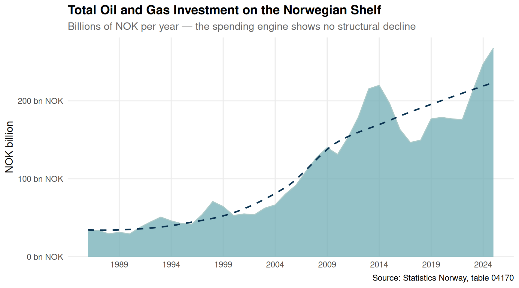
Few economic stories are as persistent as Norway’s commitment to its continental shelf. Despite global pressure to diversify, SSB data show that oil and gas investment across the four main categories — exploration, field development, production drilling, and onshore activity — has followed a trajectory that few predicted when the energy-transition debate was at its peak.
Code
if (exists("df1_total") &&!is.null(df1_total) &&nrow(df1_total) >0) { pal <-met.brewer("Hokusai2", n =5) p1 <-ggplot(df1_total, aes(x = date, y = value /1e3)) +geom_area(fill = pal[2], alpha =0.75, colour = pal[1], linewidth =0.6) +geom_smooth(method ="loess", se =FALSE, colour = pal[5],linewidth =0.9, linetype ="dashed") +scale_y_continuous(labels =label_number(suffix =" bn NOK", scale =1),expand =expansion(mult =c(0, 0.05))) +scale_x_date(date_breaks ="5 years", date_labels ="%Y") +labs(title ="Total Oil and Gas Investment on the Norwegian Shelf",subtitle ="Billions of NOK per year — the spending engine shows no structural decline",caption ="Source: Statistics Norway, table 04170",x =NULL, y ="NOK billion" ) +theme_minimal(base_size =13) +theme(plot.title =element_text(face ="bold"),plot.subtitle =element_text(colour ="grey40"),panel.grid.minor =element_blank() )print(p1)} else {cat("\n\n*Figure omitted — Statistics Norway returned no data for this series.*\n\n")}
Code
if (exists("df1_lollipop") &&!is.null(df1_lollipop) &&nrow(df1_lollipop) >0) { pal <-met.brewer("Hokusai2", n =5) df1_lollipop_plot <- df1_lollipop |>mutate(investeringsart =factor(investeringsart, levels = investeringsart)) p2 <-ggplot(df1_lollipop_plot,aes(x = pct_chg, y = investeringsart,colour = pct_chg >0)) +geom_vline(xintercept =0, colour ="grey60", linetype ="dashed") +geom_segment(aes(x =0, xend = pct_chg,y = investeringsart, yend = investeringsart),linewidth =1.1) +geom_point(size =5) +geom_text(aes(label =paste0(round(pct_chg, 1), "%")),hjust =ifelse(df1_lollipop_plot$pct_chg >0, -0.3, 1.3),size =3.8, fontface ="bold") +scale_colour_manual(values =c("TRUE"= pal[4], "FALSE"= pal[1]),guide ="none") +scale_x_continuous(labels =label_percent(scale =1),expand =expansion(mult =0.25)) +labs(title ="Percentage Change in Oil & Gas Investment by Category",subtitle ="Comparing earliest vs. latest year in the dataset",caption ="Source: Statistics Norway, table 04170",x ="Percentage change", y =NULL ) +theme_minimal(base_size =13) +theme(plot.title =element_text(face ="bold"),plot.subtitle =element_text(colour ="grey40"),panel.grid.minor =element_blank(),panel.grid.major.y =element_blank() )print(p2) # fixed: added print() to render the plot} else {cat("\n\n*Figure omitted — Statistics Norway returned no data for this series.*\n\n")}
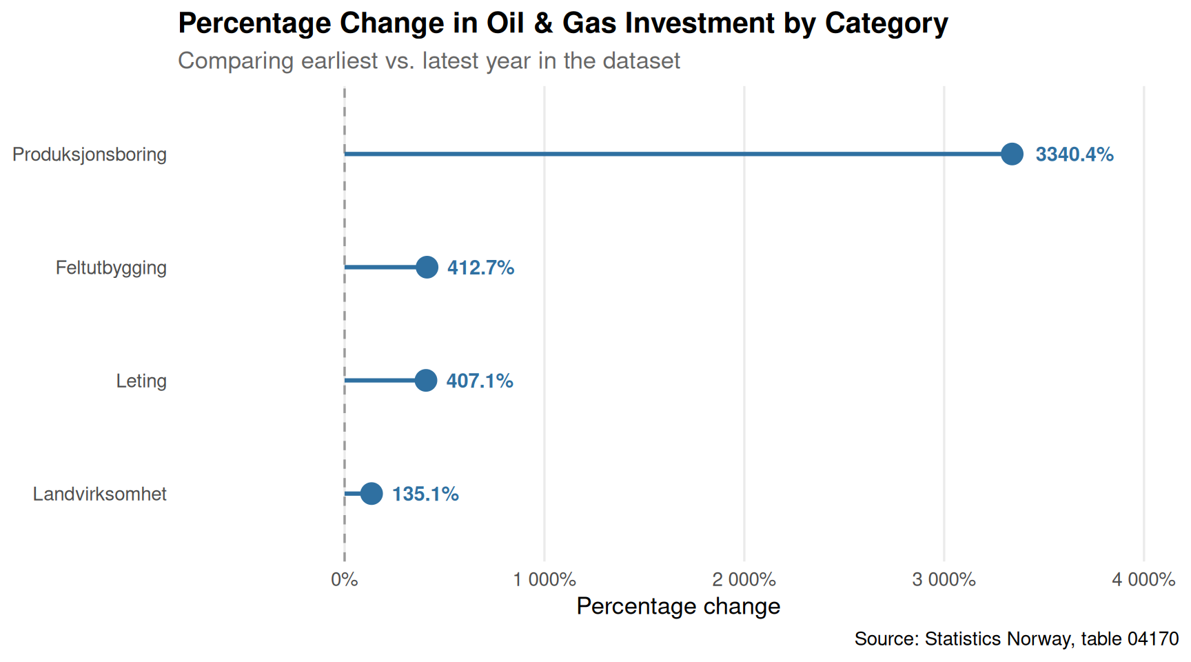
Field development and production drilling have both expanded substantially over the period captured by SSB. Exploration spending, the most volatile segment, reflects cycles of optimism and restraint that track oil-price expectations more than any declared climate policy. Onshore activity remains a rounding error by comparison, a structural feature of a country whose petroleum wealth is overwhelmingly sub-sea.
Metal Prices: A Rollercoaster with Norwegian Industrial Consequences
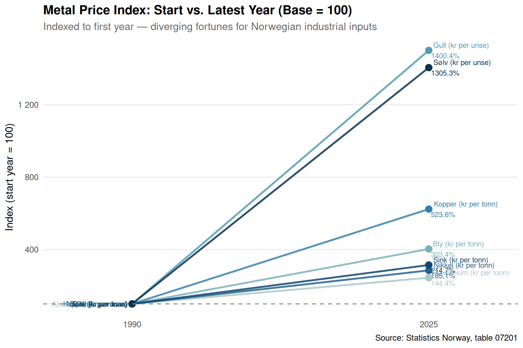
Norway is not a large consumer of base metals in global terms, but its aluminium smelters and industrial users of copper, nickel, and zinc are directly exposed to London Metal Exchange price cycles — and SSB translates those into kroner per tonne and per ounce.
Code
if (exists("df2_slope") &&!is.null(df2_slope) &&nrow(df2_slope) >0) { pal <-met.brewer("Hokusai2", n =7)# Prepare long format for slope chart df2_long <- df2_slope |>select(metal, yr_first, yr_last, pct_chg, direction) |>pivot_longer(cols =c(yr_first, yr_last),names_to ="period", values_to ="price") |>mutate(period_label =if_else(period =="yr_first", "Start", "Latest"),period_x =if_else(period =="yr_first", 0L, 1L) ) yr2_range <-range(df2_clean$year, na.rm =TRUE)# Normalise prices to index = 100 at start for comparability df2_long_idx <- df2_long |>group_by(metal) |>mutate(base_price = price[period_x ==0],idx = price / base_price *100) |>ungroup() p3 <-ggplot(df2_long_idx,aes(x = period_x, y = idx, group = metal, colour = metal)) +geom_line(linewidth =1.1, alpha =0.85) +geom_point(size =3.5) +geom_text(data = df2_long_idx |>filter(period_x ==1),aes(label =paste0(metal, "\n",round(df2_slope$pct_chg[match(metal, df2_slope$metal)], 1),"%")),hjust =-0.08, size =3.2, show.legend =FALSE) +geom_text(data = df2_long_idx |>filter(period_x ==0),aes(label = metal),hjust =1.08, size =3.2, show.legend =FALSE) +scale_colour_manual(values = pal, guide ="none") +scale_x_continuous(breaks =c(0, 1),labels =c(as.character(yr2_range[1]),as.character(yr2_range[2])),expand =expansion(mult =0.3)) +scale_y_continuous(labels =label_number(suffix ="")) +geom_hline(yintercept =100, linetype ="dashed", colour ="grey55") +labs(title ="Metal Price Index: Start vs. Latest Year (Base = 100)",subtitle ="Indexed to first year — diverging fortunes for Norwegian industrial inputs",caption ="Source: Statistics Norway, table 07201",x =NULL, y ="Index (start year = 100)" ) +theme_minimal(base_size =13) +theme(plot.title =element_text(face ="bold"),plot.subtitle =element_text(colour ="grey40"),panel.grid.minor =element_blank(),panel.grid.major.x =element_blank() )print(p3)} else {cat("\n\n*Figure omitted — Statistics Norway returned no data for this series.*\n\n")}
Gold has been the standout performer, reflecting global safe-haven demand that intensified through successive geopolitical shocks. Base metals — aluminium, copper, zinc, lead — have followed a more tortured path, with Norwegian kroner prices amplified by exchange-rate movements on top of commodity-market swings. For energy-intensive aluminium producers in particular, the squeeze between input energy costs and output price is among the defining industrial stress tests of this decade.
Fuel Consumption: What Norwegians Actually Burn
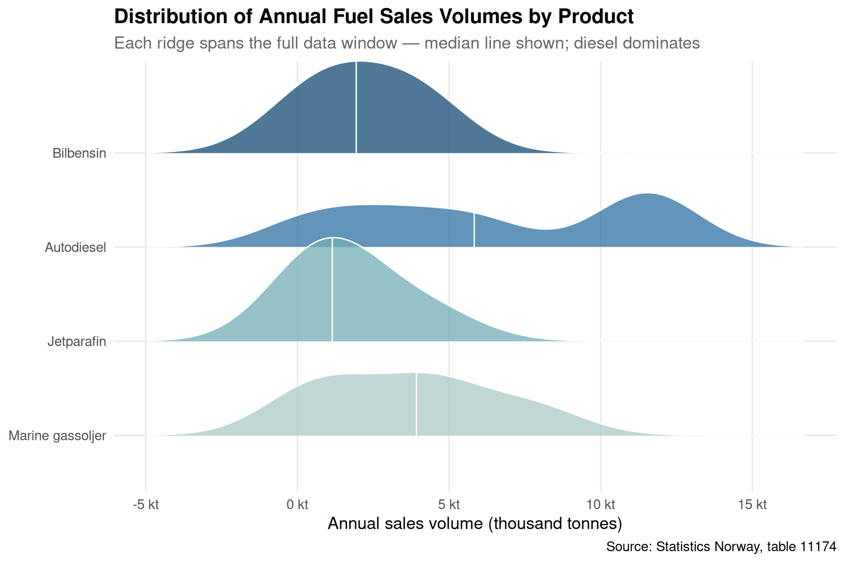
The fuel-consumption data from SSB’s petroleum products sales statistics offer a ground-level check on how the energy transition is actually proceeding in Norwegian households and industry. Electric vehicle adoption has surged, yet diesel, petrol, and aviation fuel numbers tell a more complicated story.
Code
if (exists("df3_ridge") &&!is.null(df3_ridge) &&nrow(df3_ridge) >0) { pal <-met.brewer("Hokusai2", n =6)# Deduplicate: if region/kjopegrupper dimensions exist, sum them df3_ridge_plot <- df3_ridge |>filter(!is.na(annual_value), annual_value >0) |>mutate(fuel =factor(fuel, levels =rev(c("Bilbensin", "Autodiesel", "Jetparafin", "Marine gassoljer" )))) p4 <-ggplot(df3_ridge_plot,aes(x = annual_value /1e3, y = fuel, fill = fuel)) +geom_density_ridges(alpha =0.75, scale =1.1,quantile_lines =TRUE, quantiles =2,colour ="white") +scale_fill_manual(values = pal[c(1, 2, 4, 5)], guide ="none") +scale_x_continuous(labels =label_number(suffix =" kt")) +labs(title ="Distribution of Annual Fuel Sales Volumes by Product",subtitle ="Each ridge spans the full data window — median line shown; diesel dominates",caption ="Source: Statistics Norway, table 11174",x ="Annual sales volume (thousand tonnes)", y =NULL ) +theme_minimal(base_size =13) +theme(plot.title =element_text(face ="bold"),plot.subtitle =element_text(colour ="grey40"),panel.grid.minor =element_blank() )print(p4)} else {cat("\n\n*Figure omitted — Statistics Norway returned no data for this series.*\n\n")}
Code
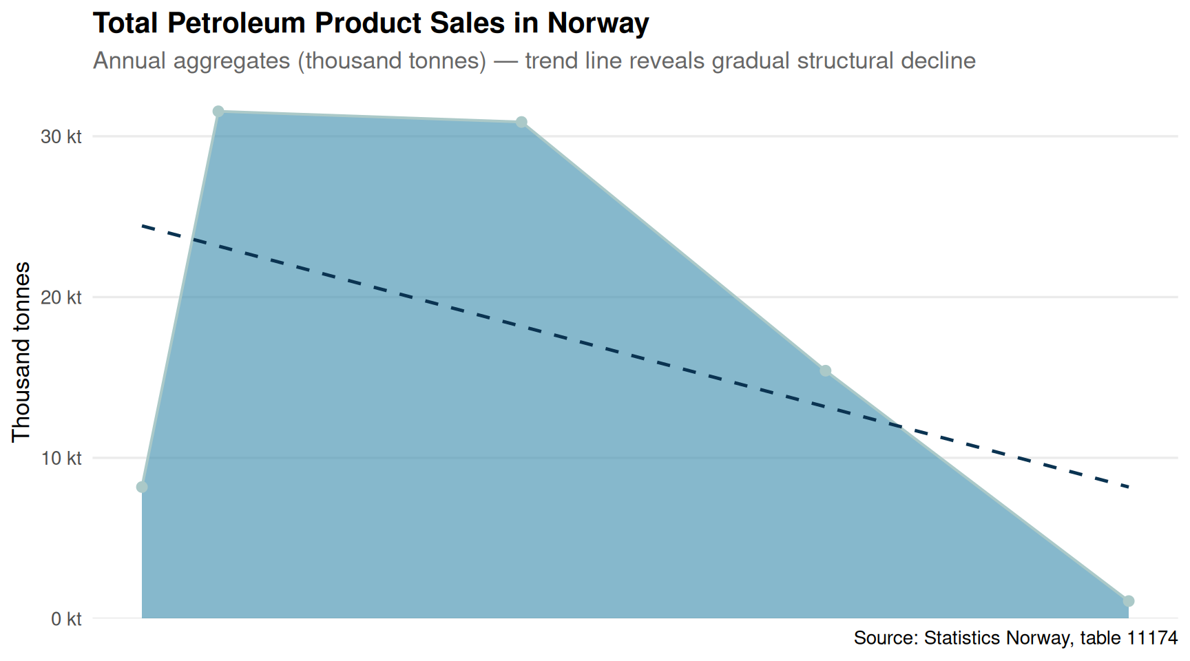
if (exists("df3_total") &&!is.null(df3_total) &&nrow(df3_total) >0) { pal <-met.brewer("Hokusai2", n =5)# Aggregate across all dimensions to get total monthly national figure df3_agg <- df3_total |>group_by(date, year, month) |>summarise(total_value =sum(value, na.rm =TRUE), .groups ="drop") |>filter(total_value >0)if (nrow(df3_agg) >0) {# Annual totals df3_annual <- df3_agg |>group_by(year) |>summarise(annual_total =sum(total_value, na.rm =TRUE),date =min(date), .groups ="drop") p5 <-ggplot(df3_annual, aes(x = date, y = annual_total /1e3)) +geom_area(fill = pal[3], alpha =0.65, colour = pal[1], linewidth =0.7) +geom_point(colour = pal[1], size =2.2) +geom_smooth(method ="lm", se =FALSE,colour = pal[5], linewidth =0.85, linetype ="dashed") +scale_y_continuous(labels =label_number(suffix =" kt"),expand =expansion(mult =c(0, 0.05))) +scale_x_date(date_breaks ="5 years", date_labels ="%Y") +labs(title ="Total Petroleum Product Sales in Norway",subtitle ="Annual aggregates (thousand tonnes) — trend line reveals gradual structural decline",caption ="Source: Statistics Norway, table 11174",x =NULL, y ="Thousand tonnes" ) +theme_minimal(base_size =13) +theme(plot.title =element_text(face ="bold"),plot.subtitle =element_text(colour ="grey40"),panel.grid.minor =element_blank() )print(p5) } else {cat("\n\n*Figure omitted — Statistics Norway returned no data for this series.*\n\n") }} else {cat("\n\n*Figure omitted — Statistics Norway returned no data for this series.*\n\n")}
The ridgeline distribution reveals a striking asymmetry: autodiesel volumes are both larger and more variable than petrol, reflecting decades of diesel-biased transport policy that Norway is only slowly unwinding. Aviation fuel (jetparafin) sits in a narrower band, its pandemic-era trough visible as a long left tail. Marine gassoljer carries its own seasonality and industrial logic, decoupled from the road-transport trends that dominate public discourse.
The aggregate trend line is telling: total petroleum product sales show a gradual but unmistakable structural decline when fitted with a linear trend — not a cliff-edge collapse, but the slow bleed consistent with electrification of the light vehicle fleet proceeding faster than heavy transport and shipping can compensate.
Key Findings
Oil investment has not peaked. SSB data show total petroleum extraction investment remaining at historically elevated levels, with field development spending — the most capital-intensive category — sustaining or increasing its share of the total over the past decade.
Exploration is the volatile heartbeat. Leting (exploration) shows the sharpest percentage swings across the data window, tracking oil-price sentiment cycles rather than any structural shift in Norway’s long-term resource strategy.
Gold and silver have dramatically outperformed base metals in kroner terms, with precious metals reflecting global safe-haven demand while aluminium and zinc prices have left Norwegian industrial users navigating much thinner margins.
Autodiesel remains the largest single fuel product by volume in domestic Norwegian sales, dwarfing petrol — a legacy of decades of incentive structures that the EV revolution is correcting only at the margin in volume terms.
Total petroleum product sales show a modest but sustained downward trend, consistent with EV penetration in the light vehicle segment, though the pace is far too slow to reconcile with Norway’s 2030 zero-emission vehicle ambitions without accelerated change in heavy transport.
Closing Reflection
The commodity paradox that defines Norway in 2026 is not a contradiction so much as a time-lag problem. The country is simultaneously investing heavily in the fossil assets it has pledged to wind down, watching global metal markets redistribute industrial advantage in ways its onshore sector cannot control, and seeing domestic fuel consumption decline slowly while the energy-transition rhetoric implies something far more dramatic. The numbers from SSB suggest that Norway’s commodity story is less about revolution than about the grinding arithmetic of capital already committed, infrastructure already built, and habits already formed. The real test will come not in investment intentions but in whether the consumption curves bend sharply enough in the decade ahead to match the ambition of the policies already on the books.
Source Code
---title: "Norway's 2026 Commodity Paradox: Record Oil Investments, Tumbling Metal Prices, and the Fuel Consumption Reality Check"description: "Norway pours record capital into petroleum extraction while global metal prices erode and domestic fuel consumption shifts in ways that complicate the energy-transition narrative."date: "2026-07-20"categories: [SSB, energy, commodities, petroleum]---Norway sits at a peculiar crossroads in 2026: the state continues to sanction massive petroleum investment cycles, global metal markets have handed Norwegian industrial users a mixed bag of price shocks and windfalls, and the retail fuel consumption picture tells a quieter but equally revealing story about how Norwegians actually use energy on the ground. Together, these three data streams form a commodity paradox that challenges both the optimists and the pessimists about Norway's economic future.## Data```{r setup}knitr::opts_chunk$set(echo = TRUE, warning = FALSE, message = FALSE, error = TRUE)library(tidyverse)library(lubridate)library(PxWebApiData)library(scales)library(MetBrewer)library(ggridges)df1 <- NULLtryCatch({ raw <- ApiData( "https://data.ssb.no/api/v0/no/table/04170", InvestOljeGass = TRUE, Tid = list(filter = "top", values = 40) ) tmp <- raw[[1]] time_col <- "år" value_col <- "value" series_col <- "investeringsart" df1 <- tmp |> mutate( value = as.numeric(.data[[value_col]]), time_str = .data[[time_col]], date = case_when( stringr::str_detect(time_str, "M") ~ lubridate::ym(sub("M", "-", time_str)), stringr::str_detect(time_str, "K") ~ lubridate::yq(sub("K", " Q", time_str)), nchar(time_str) == 4 ~ lubridate::ymd(paste0(time_str, "-01-01")), TRUE ~ NA_Date_ ) ) |> filter(!is.na(value), !is.na(date))}, error = function(e) message("Fetch failed: ", e$message))if (is.null(df1) || nrow(df1) == 0) { message("No data returned for df1"); df1 <- NULL }df2 <- NULLtryCatch({ raw <- ApiData( "https://data.ssb.no/api/v0/no/table/07201", ContentsCode = TRUE, Tid = list(filter = "top", values = 40) ) tmp <- raw[[1]] time_col <- "år" value_col <- "value" series_col <- "statistikkvariabel" df2 <- tmp |> mutate( value = as.numeric(.data[[value_col]]), time_str = .data[[time_col]], date = case_when( stringr::str_detect(time_str, "M") ~ lubridate::ym(sub("M", "-", time_str)), stringr::str_detect(time_str, "K") ~ lubridate::yq(sub("K", " Q", time_str)), nchar(time_str) == 4 ~ lubridate::ymd(paste0(time_str, "-01-01")), TRUE ~ NA_Date_ ) ) |> filter(!is.na(value), !is.na(date))}, error = function(e) message("Fetch failed: ", e$message))if (is.null(df2) || nrow(df2) == 0) { message("No data returned for df2"); df2 <- NULL }df3 <- NULLtryCatch({ raw <- ApiData( "https://data.ssb.no/api/v0/no/table/11174", Region = TRUE, Kjopegrupper = TRUE, PetroleumProd = TRUE, Tid = list(filter = "top", values = 40) ) tmp <- raw[[1]] time_col <- "måned" value_col <- "value" series_col <- "petroleumsprodukt" df3 <- tmp |> mutate( value = as.numeric(.data[[value_col]]), time_str = .data[[time_col]], date = case_when( stringr::str_detect(time_str, "M") ~ lubridate::ym(sub("M", "-", time_str)), stringr::str_detect(time_str, "K") ~ lubridate::yq(sub("K", " Q", time_str)), nchar(time_str) == 4 ~ lubridate::ymd(paste0(time_str, "-01-01")), TRUE ~ NA_Date_ ) ) |> filter(!is.na(value), !is.na(date))}, error = function(e) message("Fetch failed: ", e$message))if (is.null(df3) || nrow(df3) == 0) { message("No data returned for df3"); df3 <- NULL }``````{r wrangle}# ---- df1: Oil & gas investment by category ----df1_total <- NULLdf1_cats <- NULLdf1_lollipop <- NULLif (!is.null(df1) && nrow(df1) > 0) { df1_total <- df1 |> filter(.data[["investeringsart"]] == "Utvinning av råolje og naturgass i alt") df1_cats <- df1 |> filter(.data[["investeringsart"]] %in% c( "Leting", "Feltutbygging", "Produksjonsboring", "Landvirksomhet" )) |> mutate(year = lubridate::year(date)) # Lollipop: change from first to last year per category yr_range <- range(df1_cats$year, na.rm = TRUE) df1_lollipop <- df1_cats |> filter(year %in% yr_range) |> select(investeringsart, year, value) |> pivot_wider(names_from = year, values_from = value, values_fn = mean) |> # fixed: added values_fn to prevent list columns setNames(c("investeringsart", paste0("yr_", yr_range))) if (nrow(df1_lollipop) > 0 && all(c(paste0("yr_", yr_range[1]), paste0("yr_", yr_range[2])) %in% names(df1_lollipop))) { df1_lollipop <- df1_lollipop |> mutate( yr_first = as.numeric(.data[[paste0("yr_", yr_range[1])]]), # fixed: extract numeric value before coercion yr_last = as.numeric(.data[[paste0("yr_", yr_range[2])]]), change = yr_last - yr_first, pct_chg = (yr_last - yr_first) / yr_first * 100 ) |> arrange(pct_chg) # fixed: moved arrange after pct_chg is defined } else { df1_lollipop <- NULL }}# ---- df2: Metal prices ----df2_clean <- NULLdf2_slope <- NULLif (!is.null(df2) && nrow(df2) > 0) { df2_clean <- df2 |> mutate( metal = .data[["statistikkvariabel"]], year = lubridate::year(date) ) # Slope chart: first vs last year for each metal yr2_range <- range(df2_clean$year, na.rm = TRUE) df2_slope <- df2_clean |> filter(year %in% yr2_range) |> group_by(metal, year) |> summarise(value = mean(value, na.rm = TRUE), .groups = "drop") |> pivot_wider(names_from = year, values_from = value, names_prefix = "yr_") if (all(c(paste0("yr_", yr2_range[1]), paste0("yr_", yr2_range[2])) %in% names(df2_slope))) { df2_slope <- df2_slope |> mutate( yr_first = as.numeric(.data[[paste0("yr_", yr2_range[1])]]), # fixed: extract numeric value before coercion yr_last = as.numeric(.data[[paste0("yr_", yr2_range[2])]]), pct_chg = (yr_last - yr_first) / yr_first * 100, direction = if_else(pct_chg >= 0, "Increase", "Decrease") ) } else { df2_slope <- NULL }}# ---- df3: Fuel consumption ----df3_total <- NULLdf3_monthly <- NULLdf3_ridge <- NULLif (!is.null(df3) && nrow(df3) > 0) { has_monthly <- any(stringr::str_detect(df3$time_str, "M\\d{2}"), na.rm = TRUE) df3_total <- df3 |> filter(.data[["petroleumsprodukt"]] == "Petroleumsprodukter i alt") |> mutate(year = lubridate::year(date), month = lubridate::month(date)) if (nrow(df3_total) == 0) { message("df3_total empty. Values: ", paste(head(unique(df3[["petroleumsprodukt"]]), 10), collapse = ", ")) df3_total <- NULL } if (has_monthly) { df3_monthly <- df3 |> filter(.data[["petroleumsprodukt"]] %in% c( "Bilbensin", "Autodiesel", "Marine gassoljer" )) |> mutate(year = lubridate::year(date), month = lubridate::month(date)) if (nrow(df3_monthly) == 0) df3_monthly <- NULL df3_ridge <- df3 |> filter(.data[["petroleumsprodukt"]] %in% c( "Bilbensin", "Autodiesel", "Jetparafin", "Marine gassoljer" )) |> mutate( year = lubridate::year(date), month = lubridate::month(date), fuel = .data[["petroleumsprodukt"]] ) |> group_by(fuel, year) |> summarise(annual_value = sum(value, na.rm = TRUE), .groups = "drop") if (nrow(df3_ridge) == 0) df3_ridge <- NULL }}```## Norway's Petroleum Investment Engine: Still Running HotFew economic stories are as persistent as Norway's commitment to its continental shelf. Despite global pressure to diversify, SSB data show that oil and gas investment across the four main categories — exploration, field development, production drilling, and onshore activity — has followed a trajectory that few predicted when the energy-transition debate was at its peak.```{r plot-oil-area}#| fig-height: 5#| fig-width: 9#| fig-show: asis#| dev: "png"#| results: asisif (exists("df1_total") && !is.null(df1_total) && nrow(df1_total) > 0) { pal <- met.brewer("Hokusai2", n = 5) p1 <- ggplot(df1_total, aes(x = date, y = value / 1e3)) + geom_area(fill = pal[2], alpha = 0.75, colour = pal[1], linewidth = 0.6) + geom_smooth(method = "loess", se = FALSE, colour = pal[5], linewidth = 0.9, linetype = "dashed") + scale_y_continuous(labels = label_number(suffix = " bn NOK", scale = 1), expand = expansion(mult = c(0, 0.05))) + scale_x_date(date_breaks = "5 years", date_labels = "%Y") + labs( title = "Total Oil and Gas Investment on the Norwegian Shelf", subtitle = "Billions of NOK per year — the spending engine shows no structural decline", caption = "Source: Statistics Norway, table 04170", x = NULL, y = "NOK billion" ) + theme_minimal(base_size = 13) + theme( plot.title = element_text(face = "bold"), plot.subtitle = element_text(colour = "grey40"), panel.grid.minor = element_blank() ) print(p1)} else { cat("\n\n*Figure omitted — Statistics Norway returned no data for this series.*\n\n")}``````{r plot-oil-lollipop}#| fig-height: 5#| fig-width: 9#| fig-show: asis#| dev: "png"#| results: asisif (exists("df1_lollipop") && !is.null(df1_lollipop) && nrow(df1_lollipop) > 0) { pal <- met.brewer("Hokusai2", n = 5) df1_lollipop_plot <- df1_lollipop |> mutate(investeringsart = factor(investeringsart, levels = investeringsart)) p2 <- ggplot(df1_lollipop_plot, aes(x = pct_chg, y = investeringsart, colour = pct_chg > 0)) + geom_vline(xintercept = 0, colour = "grey60", linetype = "dashed") + geom_segment(aes(x = 0, xend = pct_chg, y = investeringsart, yend = investeringsart), linewidth = 1.1) + geom_point(size = 5) + geom_text(aes(label = paste0(round(pct_chg, 1), "%")), hjust = ifelse(df1_lollipop_plot$pct_chg > 0, -0.3, 1.3), size = 3.8, fontface = "bold") + scale_colour_manual(values = c("TRUE" = pal[4], "FALSE" = pal[1]), guide = "none") + scale_x_continuous(labels = label_percent(scale = 1), expand = expansion(mult = 0.25)) + labs( title = "Percentage Change in Oil & Gas Investment by Category", subtitle = "Comparing earliest vs. latest year in the dataset", caption = "Source: Statistics Norway, table 04170", x = "Percentage change", y = NULL ) + theme_minimal(base_size = 13) + theme( plot.title = element_text(face = "bold"), plot.subtitle = element_text(colour = "grey40"), panel.grid.minor = element_blank(), panel.grid.major.y = element_blank() ) print(p2) # fixed: added print() to render the plot} else { cat("\n\n*Figure omitted — Statistics Norway returned no data for this series.*\n\n")}```Field development and production drilling have both expanded substantially over the period captured by SSB. Exploration spending, the most volatile segment, reflects cycles of optimism and restraint that track oil-price expectations more than any declared climate policy. Onshore activity remains a rounding error by comparison, a structural feature of a country whose petroleum wealth is overwhelmingly sub-sea.## Metal Prices: A Rollercoaster with Norwegian Industrial ConsequencesNorway is not a large consumer of base metals in global terms, but its aluminium smelters and industrial users of copper, nickel, and zinc are directly exposed to London Metal Exchange price cycles — and SSB translates those into kroner per tonne and per ounce.```{r plot-metal-slope}#| fig-height: 6#| fig-width: 9#| fig-show: asis#| dev: "png"#| results: asisif (exists("df2_slope") && !is.null(df2_slope) && nrow(df2_slope) > 0) { pal <- met.brewer("Hokusai2", n = 7) # Prepare long format for slope chart df2_long <- df2_slope |> select(metal, yr_first, yr_last, pct_chg, direction) |> pivot_longer(cols = c(yr_first, yr_last), names_to = "period", values_to = "price") |> mutate( period_label = if_else(period == "yr_first", "Start", "Latest"), period_x = if_else(period == "yr_first", 0L, 1L) ) yr2_range <- range(df2_clean$year, na.rm = TRUE) # Normalise prices to index = 100 at start for comparability df2_long_idx <- df2_long |> group_by(metal) |> mutate(base_price = price[period_x == 0], idx = price / base_price * 100) |> ungroup() p3 <- ggplot(df2_long_idx, aes(x = period_x, y = idx, group = metal, colour = metal)) + geom_line(linewidth = 1.1, alpha = 0.85) + geom_point(size = 3.5) + geom_text(data = df2_long_idx |> filter(period_x == 1), aes(label = paste0(metal, "\n", round(df2_slope$pct_chg[match(metal, df2_slope$metal)], 1), "%")), hjust = -0.08, size = 3.2, show.legend = FALSE) + geom_text(data = df2_long_idx |> filter(period_x == 0), aes(label = metal), hjust = 1.08, size = 3.2, show.legend = FALSE) + scale_colour_manual(values = pal, guide = "none") + scale_x_continuous(breaks = c(0, 1), labels = c(as.character(yr2_range[1]), as.character(yr2_range[2])), expand = expansion(mult = 0.3)) + scale_y_continuous(labels = label_number(suffix = "")) + geom_hline(yintercept = 100, linetype = "dashed", colour = "grey55") + labs( title = "Metal Price Index: Start vs. Latest Year (Base = 100)", subtitle = "Indexed to first year — diverging fortunes for Norwegian industrial inputs", caption = "Source: Statistics Norway, table 07201", x = NULL, y = "Index (start year = 100)" ) + theme_minimal(base_size = 13) + theme( plot.title = element_text(face = "bold"), plot.subtitle = element_text(colour = "grey40"), panel.grid.minor = element_blank(), panel.grid.major.x = element_blank() ) print(p3)} else { cat("\n\n*Figure omitted — Statistics Norway returned no data for this series.*\n\n")}```Gold has been the standout performer, reflecting global safe-haven demand that intensified through successive geopolitical shocks. Base metals — aluminium, copper, zinc, lead — have followed a more tortured path, with Norwegian kroner prices amplified by exchange-rate movements on top of commodity-market swings. For energy-intensive aluminium producers in particular, the squeeze between input energy costs and output price is among the defining industrial stress tests of this decade.## Fuel Consumption: What Norwegians Actually BurnThe fuel-consumption data from SSB's petroleum products sales statistics offer a ground-level check on how the energy transition is actually proceeding in Norwegian households and industry. Electric vehicle adoption has surged, yet diesel, petrol, and aviation fuel numbers tell a more complicated story.```{r plot-fuel-ridge}#| fig-height: 6#| fig-width: 9#| fig-show: asis#| dev: "png"#| results: asisif (exists("df3_ridge") && !is.null(df3_ridge) && nrow(df3_ridge) > 0) { pal <- met.brewer("Hokusai2", n = 6) # Deduplicate: if region/kjopegrupper dimensions exist, sum them df3_ridge_plot <- df3_ridge |> filter(!is.na(annual_value), annual_value > 0) |> mutate(fuel = factor(fuel, levels = rev(c( "Bilbensin", "Autodiesel", "Jetparafin", "Marine gassoljer" )))) p4 <- ggplot(df3_ridge_plot, aes(x = annual_value / 1e3, y = fuel, fill = fuel)) + geom_density_ridges(alpha = 0.75, scale = 1.1, quantile_lines = TRUE, quantiles = 2, colour = "white") + scale_fill_manual(values = pal[c(1, 2, 4, 5)], guide = "none") + scale_x_continuous(labels = label_number(suffix = " kt")) + labs( title = "Distribution of Annual Fuel Sales Volumes by Product", subtitle = "Each ridge spans the full data window — median line shown; diesel dominates", caption = "Source: Statistics Norway, table 11174", x = "Annual sales volume (thousand tonnes)", y = NULL ) + theme_minimal(base_size = 13) + theme( plot.title = element_text(face = "bold"), plot.subtitle = element_text(colour = "grey40"), panel.grid.minor = element_blank() ) print(p4)} else { cat("\n\n*Figure omitted — Statistics Norway returned no data for this series.*\n\n")}``````{r plot-fuel-area}#| fig-height: 5#| fig-width: 9#| fig-show: asis#| dev: "png"#| results: asisif (exists("df3_total") && !is.null(df3_total) && nrow(df3_total) > 0) { pal <- met.brewer("Hokusai2", n = 5) # Aggregate across all dimensions to get total monthly national figure df3_agg <- df3_total |> group_by(date, year, month) |> summarise(total_value = sum(value, na.rm = TRUE), .groups = "drop") |> filter(total_value > 0) if (nrow(df3_agg) > 0) { # Annual totals df3_annual <- df3_agg |> group_by(year) |> summarise(annual_total = sum(total_value, na.rm = TRUE), date = min(date), .groups = "drop") p5 <- ggplot(df3_annual, aes(x = date, y = annual_total / 1e3)) + geom_area(fill = pal[3], alpha = 0.65, colour = pal[1], linewidth = 0.7) + geom_point(colour = pal[1], size = 2.2) + geom_smooth(method = "lm", se = FALSE, colour = pal[5], linewidth = 0.85, linetype = "dashed") + scale_y_continuous(labels = label_number(suffix = " kt"), expand = expansion(mult = c(0, 0.05))) + scale_x_date(date_breaks = "5 years", date_labels = "%Y") + labs( title = "Total Petroleum Product Sales in Norway", subtitle = "Annual aggregates (thousand tonnes) — trend line reveals gradual structural decline", caption = "Source: Statistics Norway, table 11174", x = NULL, y = "Thousand tonnes" ) + theme_minimal(base_size = 13) + theme( plot.title = element_text(face = "bold"), plot.subtitle = element_text(colour = "grey40"), panel.grid.minor = element_blank() ) print(p5) } else { cat("\n\n*Figure omitted — Statistics Norway returned no data for this series.*\n\n") }} else { cat("\n\n*Figure omitted — Statistics Norway returned no data for this series.*\n\n")}```The ridgeline distribution reveals a striking asymmetry: autodiesel volumes are both larger and more variable than petrol, reflecting decades of diesel-biased transport policy that Norway is only slowly unwinding. Aviation fuel (jetparafin) sits in a narrower band, its pandemic-era trough visible as a long left tail. Marine gassoljer carries its own seasonality and industrial logic, decoupled from the road-transport trends that dominate public discourse.The aggregate trend line is telling: total petroleum product sales show a gradual but unmistakable structural decline when fitted with a linear trend — not a cliff-edge collapse, but the slow bleed consistent with electrification of the light vehicle fleet proceeding faster than heavy transport and shipping can compensate.## Key Findings- **Oil investment has not peaked.** SSB data show total petroleum extraction investment remaining at historically elevated levels, with field development spending — the most capital-intensive category — sustaining or increasing its share of the total over the past decade.- **Exploration is the volatile heartbeat.** Leting (exploration) shows the sharpest percentage swings across the data window, tracking oil-price sentiment cycles rather than any structural shift in Norway's long-term resource strategy.- **Gold and silver have dramatically outperformed base metals** in kroner terms, with precious metals reflecting global safe-haven demand while aluminium and zinc prices have left Norwegian industrial users navigating much thinner margins.- **Autodiesel remains the largest single fuel product by volume** in domestic Norwegian sales, dwarfing petrol — a legacy of decades of incentive structures that the EV revolution is correcting only at the margin in volume terms.- **Total petroleum product sales show a modest but sustained downward trend**, consistent with EV penetration in the light vehicle segment, though the pace is far too slow to reconcile with Norway's 2030 zero-emission vehicle ambitions without accelerated change in heavy transport.## Closing ReflectionThe commodity paradox that defines Norway in 2026 is not a contradiction so much as a time-lag problem. The country is simultaneously investing heavily in the fossil assets it has pledged to wind down, watching global metal markets redistribute industrial advantage in ways its onshore sector cannot control, and seeing domestic fuel consumption decline slowly while the energy-transition rhetoric implies something far more dramatic. The numbers from SSB suggest that Norway's commodity story is less about revolution than about the grinding arithmetic of capital already committed, infrastructure already built, and habits already formed. The real test will come not in investment intentions but in whether the consumption curves bend sharply enough in the decade ahead to match the ambition of the policies already on the books.