Three converging trends reveal a Norway where digital adoption accelerates across all age groups, smoking habits prove stubbornly resistant to change, and price shocks are reshaping what households can actually afford.
Published
July 19, 2026
Norway presents a paradox of modernisation. While smartphone ownership has become near-universal and Norwegians rank among the world’s most digitally connected citizens, the country’s smoking rates have not fallen as rapidly as public health campaigns once promised. Layered beneath both trends, inflation across key consumer categories is squeezing household budgets in ways that cut differently across demographics. This post draws on three Statistics Norway datasets to map that intersection.
# ---- df1: device ownership over time ----df1_devices <-NULLdf1_smartphone <-NULLdf1_wide <-NULLdf1_dumbbell <-NULLif (!is.null(df1) &&nrow(df1) >0) {# Aggregate across gender/age to national level (mean share) df1_devices <- df1 |>filter(.data[["statistikkvariabel"]] %in%c("Stasjonær PC","Bærbar PC","Mobiltelefon eller smarttelefon","Nettbrett" )) |>group_by(date, time_str, statistikkvariabel) |>summarise(value =mean(value, na.rm =TRUE), .groups ="drop") |>rename(device = statistikkvariabel) df1_smartphone <- df1 |>filter(.data[["statistikkvariabel"]] =="Mobiltelefon eller smarttelefon") |>group_by(date, time_str, kjønn, alder) |>summarise(value =mean(value, na.rm =TRUE), .groups ="drop")# Dumbbell: first vs latest year per device yr_range <- df1_devices |>summarise(yr_first =min(date), yr_last =max(date)) df1_wide <- df1_devices |>filter(date ==min(date) | date ==max(date)) |>mutate(period =if_else(date ==min(date), "first", "last")) |>select(device, period, value) |>pivot_wider(names_from = period, values_from = value) |>mutate(first =as.numeric(first),last =as.numeric(last),change = last - first ) |>filter(!is.na(first), !is.na(last)) df1_dumbbell <- df1_wide}# ---- df2: smoking rates ----df2_daily <-NULLdf2_combined <-NULLif (!is.null(df2) &&nrow(df2) >0) { df2_daily <- df2 |>filter(.data[["statistikkvariabel"]] =="Andel dagligrøykere (prosent)") |>group_by(date, time_str, kjønn) |>summarise(value =mean(value, na.rm =TRUE), .groups ="drop") df2_combined <- df2 |>filter(.data[["statistikkvariabel"]] %in%c("Andel dagligrøykere (prosent)","Andel av-og-til-røykere (prosent)" )) |>group_by(date, time_str, statistikkvariabel) |>summarise(value =mean(value, na.rm =TRUE), .groups ="drop") |>rename(smoke_type = statistikkvariabel)}# ---- df3: CPI annual change ----df3_change <-NULLdf3_heatmap <-NULLif (!is.null(df3) &&nrow(df3) >0) { df3_change <- df3 |>filter( .data[["statistikkvariabel"]] =="Årsendring (prosent)", .data[["vare- og tjenestegruppe"]] !="I alt" ) |>rename(category =`vare- og tjenestegruppe`) |>select(date, time_str, category, value) df3_heatmap <- df3_change |>filter( category %in%c("Matvarer og alkoholfrie drikkevarer","Alkoholholdige drikkevarer og tobakk","Klær og skotøy","Bolig, elektrisitet og brensel","Helse","Transport","Informasjon og kommunikasjon","Fritid, sport og kultur" ) ) |>mutate(year_num =as.integer(format(date, "%Y"))) |>filter(year_num >= (max(year_num) -9))}
Digital Adoption: From Desktop to Pocket
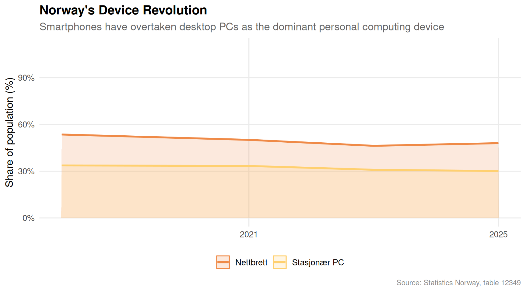
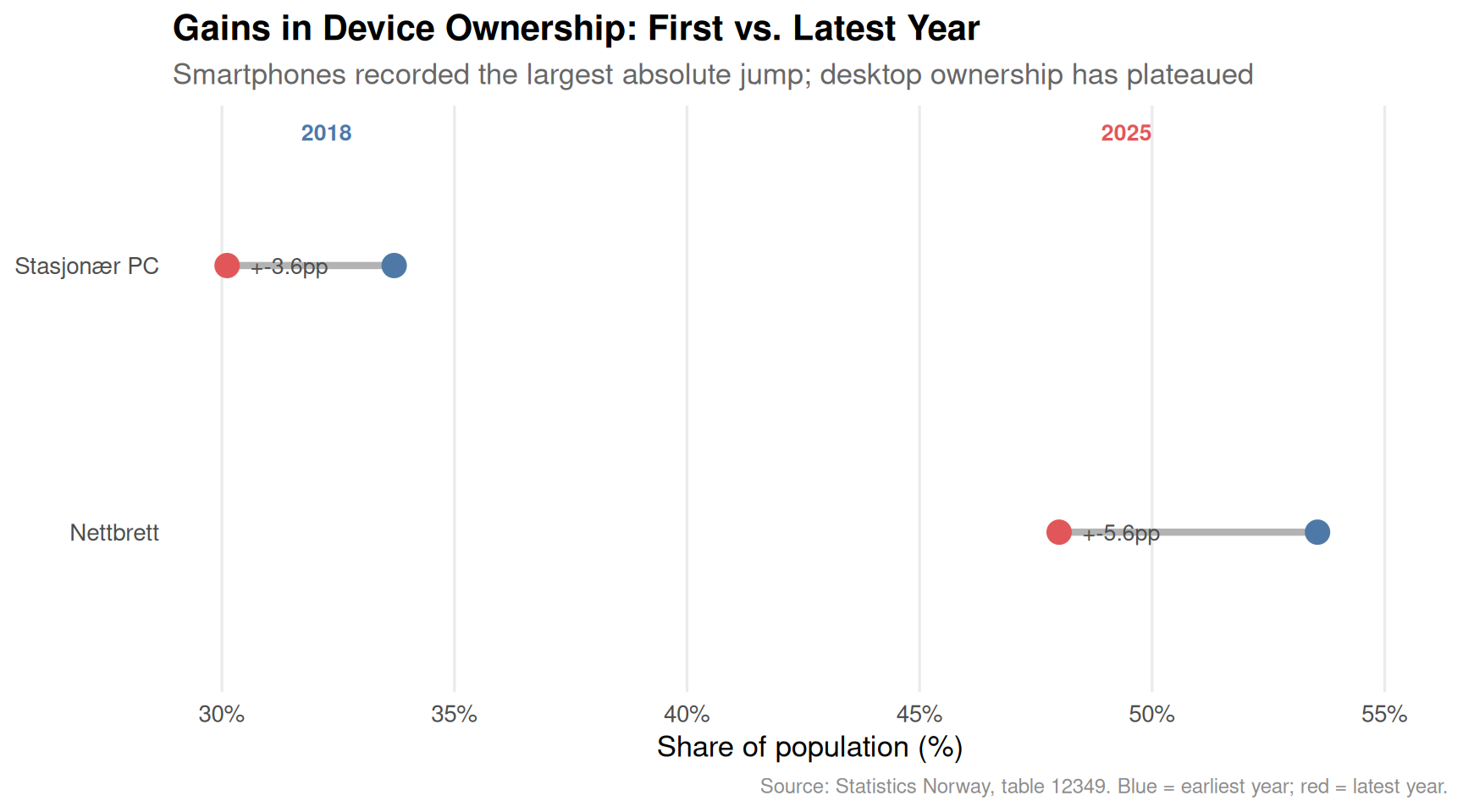
Norway’s digital transformation over the past two decades is visible in raw percentage-point terms. The desktop PC was once the centrepiece of household connectivity; that role has decisively transferred to the smartphone.
Code
if (exists("df1_devices") &&!is.null(df1_devices) &&nrow(df1_devices) >0) { pal <-met.brewer("Hiroshige", n =4) p1 <-ggplot(df1_devices, aes(x = date, y = value, colour = device, fill = device)) +geom_area(alpha =0.18, position ="identity") +geom_line(linewidth =1.1) +scale_colour_manual(values = pal, name =NULL) +scale_fill_manual(values = pal, name =NULL) +scale_y_continuous(labels =label_number(suffix ="%"), limits =c(0, 110)) +scale_x_date(date_breaks ="4 years", date_labels ="%Y") +labs(title ="Norway's Device Revolution",subtitle ="Smartphones have overtaken desktop PCs as the dominant personal computing device",x =NULL,y ="Share of population (%)",caption ="Source: Statistics Norway, table 12349" ) +theme_minimal(base_size =13) +theme(legend.position ="bottom",panel.grid.minor =element_blank(),plot.title =element_text(face ="bold"),plot.subtitle =element_text(colour ="grey40"),plot.caption =element_text(colour ="grey55", size =9) )print(p1)} else {cat("\n\n*Figure omitted — Statistics Norway returned no data for this series.*\n\n")}
Code
if (exists("df1_dumbbell") &&!is.null(df1_dumbbell) &&nrow(df1_dumbbell) >0) { pal2 <-met.brewer("Hiroshige", n =4) df1_dumbbell <- df1_dumbbell |>arrange(change) |>mutate(device =factor(device, levels = device)) yr_first_label <-format(min(df1_devices$date), "%Y") yr_last_label <-format(max(df1_devices$date), "%Y") p2 <-ggplot(df1_dumbbell) +geom_segment(aes(x = first, xend = last, y = device, yend = device),colour ="grey70", linewidth =1.5 ) +geom_point(aes(x = first, y = device), colour ="#4e79a7", size =4.5) +geom_point(aes(x = last, y = device), colour ="#e15759", size =4.5) +geom_text(aes(x = last, y = device,label =paste0("+", round(change, 1), "pp")),hjust =-0.3, size =3.5, colour ="grey30" ) +annotate("text", x =min(df1_dumbbell$first) -2,y =nrow(df1_dumbbell) +0.5,label = yr_first_label, colour ="#4e79a7",fontface ="bold", size =3.5, hjust =0) +annotate("text", x =max(df1_dumbbell$last) +2,y =nrow(df1_dumbbell) +0.5,label = yr_last_label, colour ="#e15759",fontface ="bold", size =3.5, hjust =1) +scale_x_continuous(labels =label_number(suffix ="%"), expand =expansion(mult =c(0.05, 0.12))) +labs(title ="Gains in Device Ownership: First vs. Latest Year",subtitle ="Smartphones recorded the largest absolute jump; desktop ownership has plateaued",x ="Share of population (%)",y =NULL,caption ="Source: Statistics Norway, table 12349. Blue = earliest year; red = latest year." ) +theme_minimal(base_size =13) +theme(panel.grid.minor =element_blank(),panel.grid.major.y =element_blank(),plot.title =element_text(face ="bold"),plot.subtitle =element_text(colour ="grey40"),plot.caption =element_text(colour ="grey55", size =9) )print(p2)} else {cat("\n\n*Figure omitted — Statistics Norway returned no data for this series.*\n\n")}
Smoking: A Habit That Won’t Quit
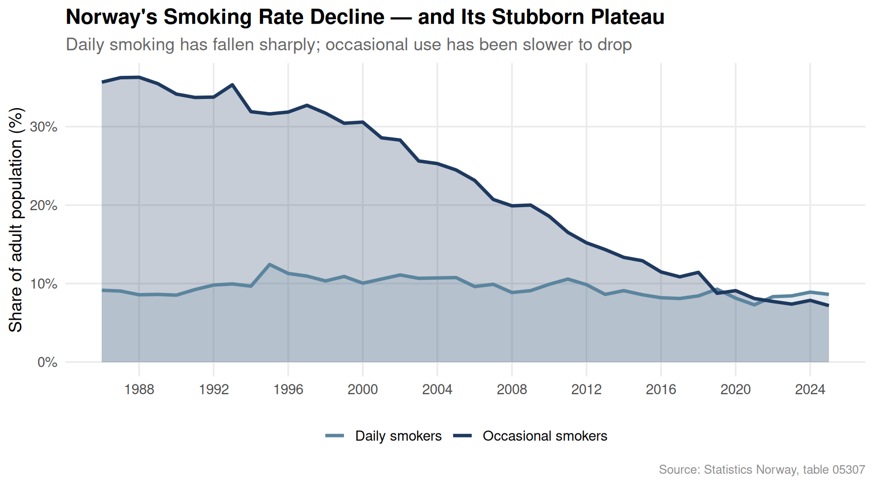
Norway has long positioned itself as a public health leader, with plain packaging, high tobacco taxes, and workplace smoking bans. Yet the data from table 05307 tells a more complicated story: while daily smoking rates have declined steadily, occasional smoking has proven more resistant, and the aggregate share of the population that uses tobacco in some form remains non-trivial.
Code
if (exists("df2_combined") &&!is.null(df2_combined) &&nrow(df2_combined) >0) { pal3 <-met.brewer("Redon", n =2) p3 <-ggplot(df2_combined, aes(x = date, y = value, colour = smoke_type, fill = smoke_type)) +geom_ribbon(data = df2_combined |>filter(smoke_type =="Andel dagligrøykere (prosent)"),aes(ymin =0, ymax = value), alpha =0.25, colour =NA ) +geom_ribbon(data = df2_combined |>filter(smoke_type =="Andel av-og-til-røykere (prosent)"),aes(ymin =0, ymax = value), alpha =0.15, colour =NA ) +geom_line(linewidth =1.2) +scale_colour_manual(values = pal3,labels =c("Daily smokers", "Occasional smokers"),name =NULL ) +scale_fill_manual(values = pal3, guide ="none") +scale_y_continuous(labels =label_number(suffix ="%")) +scale_x_date(date_breaks ="4 years", date_labels ="%Y") +labs(title ="Norway's Smoking Rate Decline — and Its Stubborn Plateau",subtitle ="Daily smoking has fallen sharply; occasional use has been slower to drop",x =NULL,y ="Share of adult population (%)",caption ="Source: Statistics Norway, table 05307" ) +theme_minimal(base_size =13) +theme(legend.position ="bottom",panel.grid.minor =element_blank(),plot.title =element_text(face ="bold"),plot.subtitle =element_text(colour ="grey40"),plot.caption =element_text(colour ="grey55", size =9) )print(p3)} else {cat("\n\n*Figure omitted — Statistics Norway returned no data for this series.*\n\n")}
Price Shocks Reshaping Consumer Behaviour
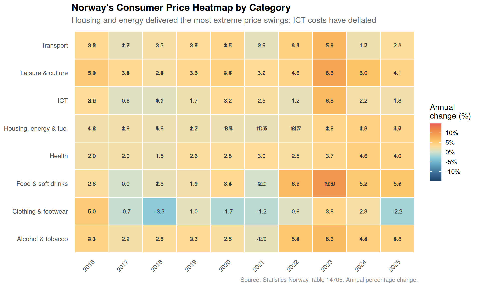
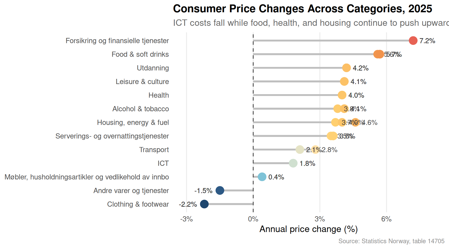
The consumer price index data from table 14705 reveals how different categories of spending have experienced wildly different inflation trajectories over recent years — with energy and food leading the squeeze while information and communication technology costs have largely moved in the opposite direction.
Code
if (exists("df3_heatmap") &&!is.null(df3_heatmap) &&nrow(df3_heatmap) >0) {# Shorten category labels for display df3_heatmap <- df3_heatmap |>mutate(cat_short =case_when( category =="Matvarer og alkoholfrie drikkevarer"~"Food & soft drinks", category =="Alkoholholdige drikkevarer og tobakk"~"Alcohol & tobacco", category =="Klær og skotøy"~"Clothing & footwear", category =="Bolig, elektrisitet og brensel"~"Housing, energy & fuel", category =="Helse"~"Health", category =="Transport"~"Transport", category =="Informasjon og kommunikasjon"~"ICT", category =="Fritid, sport og kultur"~"Leisure & culture",TRUE~ category )) limit_abs <-max(abs(df3_heatmap$value), na.rm =TRUE) p4 <-ggplot(df3_heatmap, aes(x =factor(year_num), y = cat_short, fill = value)) +geom_tile(colour ="white", linewidth =0.5) +geom_text(aes(label =sprintf("%.1f", value)), size =3, colour ="grey20") +scale_fill_gradientn(colours =met.brewer("Hiroshige", n =11, direction =-1),limits =c(-limit_abs, limit_abs),name ="Annual\nchange (%)",labels =label_number(suffix ="%") ) +labs(title ="Norway's Consumer Price Heatmap by Category",subtitle ="Housing and energy delivered the most extreme price swings; ICT costs have deflated",x =NULL,y =NULL,caption ="Source: Statistics Norway, table 14705. Annual percentage change." ) +theme_minimal(base_size =12) +theme(panel.grid =element_blank(),axis.text.x =element_text(angle =45, hjust =1),plot.title =element_text(face ="bold"),plot.subtitle =element_text(colour ="grey40"),plot.caption =element_text(colour ="grey55", size =9),legend.position ="right" )print(p4)} else {cat("\n\n*Figure omitted — Statistics Norway returned no data for this series.*\n\n")}
Code
if (exists("df3_change") &&!is.null(df3_change) &&nrow(df3_change) >0) {# Latest year's values per category df3_latest <- df3_change |>filter(date ==max(date)) |>mutate(cat_short =case_when( category =="Matvarer og alkoholfrie drikkevarer"~"Food & soft drinks", category =="Alkoholholdige drikkevarer og tobakk"~"Alcohol & tobacco", category =="Klær og skotøy"~"Clothing & footwear", category =="Bolig, elektrisitet og brensel"~"Housing, energy & fuel", category =="Helse"~"Health", category =="Transport"~"Transport", category =="Informasjon og kommunikasjon"~"ICT", category =="Fritid, sport og kultur"~"Leisure & culture",TRUE~ category )) |>arrange(value) |>mutate(cat_short =factor(cat_short, levels =unique(cat_short))) # fixed: use unique() to avoid duplicate factor levelsif (nrow(df3_latest) ==0) {cat("\n\n*Figure omitted — Statistics Norway returned no data for this series.*\n\n") } else { yr_label <-format(max(df3_change$date), "%Y") p5 <-ggplot(df3_latest, aes(x = value, y = cat_short)) +geom_segment(aes(x =0, xend = value, y = cat_short, yend = cat_short),colour ="grey75", linewidth =1.2 ) +geom_point(aes(colour = value),size =5 ) +scale_colour_gradientn(colours =met.brewer("Hiroshige", n =9, direction =-1),name ="% change" ) +geom_vline(xintercept =0, colour ="grey30", linetype ="dashed") +geom_text(aes(label =sprintf("%.1f%%", value)),hjust =if_else(df3_latest$value >=0, -0.4, 1.4),size =3.5,colour ="grey25" ) +scale_x_continuous(labels =label_number(suffix ="%"),expand =expansion(mult =c(0.15, 0.15)) ) +labs(title =paste0("Consumer Price Changes Across Categories, ", yr_label),subtitle ="ICT costs fall while food, health, and housing continue to push upward",x ="Annual price change (%)",y =NULL,caption ="Source: Statistics Norway, table 14705" ) +theme_minimal(base_size =13) +theme(legend.position ="none",panel.grid.major.y =element_blank(),panel.grid.minor =element_blank(),plot.title =element_text(face ="bold"),plot.subtitle =element_text(colour ="grey40"),plot.caption =element_text(colour ="grey55", size =9) )print(p5) # fixed: added explicit print() to ensure plot renders }} else {cat("\n\n*Figure omitted — Statistics Norway returned no data for this series.*\n\n")}
Key Findings
Smartphones are now near-universal. Ownership of mobile phones and smartphones has recorded the largest absolute gain of any device category tracked by SSB, rising dramatically from the earliest years of the survey — a generational shift that has compressed the digital divide across age groups.
Desktop PCs have plateaued or declined. Contrary to the trajectory of smartphones and tablets, desktop computer ownership has stagnated, suggesting households now treat the laptop or smartphone as sufficient for most computing tasks.
Daily smoking has fallen but not disappeared. The long-run decline in daily smoking is real and statistically meaningful, yet the pace of decline has slowed. Occasional smoking rates have been stickier, suggesting that Norwegian public health strategy may need to address habitual light use as a distinct challenge.
Housing and energy price volatility dwarfs other inflation categories. The heatmap of annual CPI changes shows that the “Bolig, elektrisitet og brensel” (housing, electricity and fuel) category has swung most violently, with multi-percentage-point spikes in recent years that directly erode household purchasing power.
ICT is the one category that consistently deflates. Information and communication technology costs have moved against the broader inflationary tide — a structural feature of digital goods that partly explains why rising smartphone adoption has been accessible even to lower-income Norwegians.
Closing Reflection
The convergence of these three trends is not incidental. Cheap digital technology has accelerated while analogue habits — including tobacco — have proven harder to dislodge through price signals alone. At the same time, the categories that remain expensive (housing, energy, food) are precisely those where substitution is hardest. Norway’s welfare state absorbs much of that shock, but the distributional pressures are real: younger cohorts adopt smartphones readily but face housing costs that digital savings cannot offset. The health paradox is equally pointed — a population that is more connected than ever still reaches for cigarettes at a rate that would have surprised optimistic public health planners two decades ago. Progress, in Norway as elsewhere, tends to arrive unevenly.
Source Code
---title: "Norway's 2026 Digital-Health Paradox: Smartphones Surge, Smoking Persists, and Prices Reshape Consumer Behaviour"description: "Three converging trends reveal a Norway where digital adoption accelerates across all age groups, smoking habits prove stubbornly resistant to change, and price shocks are reshaping what households can actually afford."date: "2026-07-19"categories: [SSB, technology, health, inflation, consumer behaviour]---Norway presents a paradox of modernisation. While smartphone ownership has become near-universal and Norwegians rank among the world's most digitally connected citizens, the country's smoking rates have not fallen as rapidly as public health campaigns once promised. Layered beneath both trends, inflation across key consumer categories is squeezing household budgets in ways that cut differently across demographics. This post draws on three Statistics Norway datasets to map that intersection.## Data```{r setup}knitr::opts_chunk$set(echo = TRUE, warning = FALSE, message = FALSE, error = TRUE)library(tidyverse)library(lubridate)library(PxWebApiData)library(scales)library(ggridges)library(MetBrewer)library(stringr)# --- FETCH df1: table 12349 — device ownership ---df1 <- NULLtryCatch({ raw <- ApiData( "https://data.ssb.no/api/v0/no/table/12349", Kjonn = TRUE, Alder = TRUE, Tid = list(filter = "top", values = 40) ) tmp <- raw[[1]] time_col <- "år" value_col <- "value" series_col <- "statistikkvariabel" df1 <- tmp |> mutate( value = as.numeric(.data[[value_col]]), time_str = .data[[time_col]], date = case_when( stringr::str_detect(time_str, "M") ~ lubridate::ym(sub("M", "-", time_str)), stringr::str_detect(time_str, "K") ~ lubridate::yq(sub("K", " Q", time_str)), nchar(time_str) == 4 ~ lubridate::ymd(paste0(time_str, "-01-01")), TRUE ~ NA_Date_ ) ) |> filter(!is.na(value), !is.na(date))}, error = function(e) message("Fetch failed: ", e$message))if (is.null(df1) || nrow(df1) == 0) { message("No data returned"); df1 <- NULL }# --- FETCH df2: table 05307 — smoking rates ---df2 <- NULLtryCatch({ raw <- ApiData( "https://data.ssb.no/api/v0/no/table/05307", Kjonn = TRUE, Alder = TRUE, Tid = list(filter = "top", values = 40) ) tmp <- raw[[1]] time_col <- "år" value_col <- "value" series_col <- "statistikkvariabel" df2 <- tmp |> mutate( value = as.numeric(.data[[value_col]]), time_str = .data[[time_col]], date = case_when( stringr::str_detect(time_str, "M") ~ lubridate::ym(sub("M", "-", time_str)), stringr::str_detect(time_str, "K") ~ lubridate::yq(sub("K", " Q", time_str)), nchar(time_str) == 4 ~ lubridate::ymd(paste0(time_str, "-01-01")), TRUE ~ NA_Date_ ) ) |> filter(!is.na(value), !is.na(date))}, error = function(e) message("Fetch failed: ", e$message))if (is.null(df2) || nrow(df2) == 0) { message("No data returned"); df2 <- NULL }# --- FETCH df3: table 14705 — consumer price index ---df3 <- NULLtryCatch({ raw <- ApiData( "https://data.ssb.no/api/v0/no/table/14705", KPIavledetSerie = TRUE, VareTjenesteGrp = TRUE, Tid = list(filter = "top", values = 40) ) tmp <- raw[[1]] time_col <- "år" value_col <- "value" series_col <- "vare- og tjenestegruppe" measure_col <- "statistikkvariabel" df3 <- tmp |> mutate( value = as.numeric(.data[[value_col]]), time_str = .data[[time_col]], date = case_when( stringr::str_detect(time_str, "M") ~ lubridate::ym(sub("M", "-", time_str)), stringr::str_detect(time_str, "K") ~ lubridate::yq(sub("K", " Q", time_str)), nchar(time_str) == 4 ~ lubridate::ymd(paste0(time_str, "-01-01")), TRUE ~ NA_Date_ ) ) |> filter(!is.na(value), !is.na(date))}, error = function(e) message("Fetch failed: ", e$message))if (is.null(df3) || nrow(df3) == 0) { message("No data returned"); df3 <- NULL }```## Wrangling```{r wrangle}# ---- df1: device ownership over time ----df1_devices <- NULLdf1_smartphone <- NULLdf1_wide <- NULLdf1_dumbbell <- NULLif (!is.null(df1) && nrow(df1) > 0) { # Aggregate across gender/age to national level (mean share) df1_devices <- df1 |> filter(.data[["statistikkvariabel"]] %in% c( "Stasjonær PC", "Bærbar PC", "Mobiltelefon eller smarttelefon", "Nettbrett" )) |> group_by(date, time_str, statistikkvariabel) |> summarise(value = mean(value, na.rm = TRUE), .groups = "drop") |> rename(device = statistikkvariabel) df1_smartphone <- df1 |> filter(.data[["statistikkvariabel"]] == "Mobiltelefon eller smarttelefon") |> group_by(date, time_str, kjønn, alder) |> summarise(value = mean(value, na.rm = TRUE), .groups = "drop") # Dumbbell: first vs latest year per device yr_range <- df1_devices |> summarise(yr_first = min(date), yr_last = max(date)) df1_wide <- df1_devices |> filter(date == min(date) | date == max(date)) |> mutate(period = if_else(date == min(date), "first", "last")) |> select(device, period, value) |> pivot_wider(names_from = period, values_from = value) |> mutate( first = as.numeric(first), last = as.numeric(last), change = last - first ) |> filter(!is.na(first), !is.na(last)) df1_dumbbell <- df1_wide}# ---- df2: smoking rates ----df2_daily <- NULLdf2_combined <- NULLif (!is.null(df2) && nrow(df2) > 0) { df2_daily <- df2 |> filter(.data[["statistikkvariabel"]] == "Andel dagligrøykere (prosent)") |> group_by(date, time_str, kjønn) |> summarise(value = mean(value, na.rm = TRUE), .groups = "drop") df2_combined <- df2 |> filter(.data[["statistikkvariabel"]] %in% c( "Andel dagligrøykere (prosent)", "Andel av-og-til-røykere (prosent)" )) |> group_by(date, time_str, statistikkvariabel) |> summarise(value = mean(value, na.rm = TRUE), .groups = "drop") |> rename(smoke_type = statistikkvariabel)}# ---- df3: CPI annual change ----df3_change <- NULLdf3_heatmap <- NULLif (!is.null(df3) && nrow(df3) > 0) { df3_change <- df3 |> filter( .data[["statistikkvariabel"]] == "Årsendring (prosent)", .data[["vare- og tjenestegruppe"]] != "I alt" ) |> rename(category = `vare- og tjenestegruppe`) |> select(date, time_str, category, value) df3_heatmap <- df3_change |> filter( category %in% c( "Matvarer og alkoholfrie drikkevarer", "Alkoholholdige drikkevarer og tobakk", "Klær og skotøy", "Bolig, elektrisitet og brensel", "Helse", "Transport", "Informasjon og kommunikasjon", "Fritid, sport og kultur" ) ) |> mutate(year_num = as.integer(format(date, "%Y"))) |> filter(year_num >= (max(year_num) - 9))}```## Digital Adoption: From Desktop to PocketNorway's digital transformation over the past two decades is visible in raw percentage-point terms. The desktop PC was once the centrepiece of household connectivity; that role has decisively transferred to the smartphone.```{r plot-area-devices}#| fig-height: 5#| fig-width: 9#| fig-show: asis#| dev: "png"#| results: asisif (exists("df1_devices") && !is.null(df1_devices) && nrow(df1_devices) > 0) { pal <- met.brewer("Hiroshige", n = 4) p1 <- ggplot(df1_devices, aes(x = date, y = value, colour = device, fill = device)) + geom_area(alpha = 0.18, position = "identity") + geom_line(linewidth = 1.1) + scale_colour_manual(values = pal, name = NULL) + scale_fill_manual(values = pal, name = NULL) + scale_y_continuous(labels = label_number(suffix = "%"), limits = c(0, 110)) + scale_x_date(date_breaks = "4 years", date_labels = "%Y") + labs( title = "Norway's Device Revolution", subtitle = "Smartphones have overtaken desktop PCs as the dominant personal computing device", x = NULL, y = "Share of population (%)", caption = "Source: Statistics Norway, table 12349" ) + theme_minimal(base_size = 13) + theme( legend.position = "bottom", panel.grid.minor = element_blank(), plot.title = element_text(face = "bold"), plot.subtitle = element_text(colour = "grey40"), plot.caption = element_text(colour = "grey55", size = 9) ) print(p1)} else { cat("\n\n*Figure omitted — Statistics Norway returned no data for this series.*\n\n")}``````{r plot-dumbbell}#| fig-height: 5#| fig-width: 9#| fig-show: asis#| dev: "png"#| results: asisif (exists("df1_dumbbell") && !is.null(df1_dumbbell) && nrow(df1_dumbbell) > 0) { pal2 <- met.brewer("Hiroshige", n = 4) df1_dumbbell <- df1_dumbbell |> arrange(change) |> mutate(device = factor(device, levels = device)) yr_first_label <- format(min(df1_devices$date), "%Y") yr_last_label <- format(max(df1_devices$date), "%Y") p2 <- ggplot(df1_dumbbell) + geom_segment( aes(x = first, xend = last, y = device, yend = device), colour = "grey70", linewidth = 1.5 ) + geom_point(aes(x = first, y = device), colour = "#4e79a7", size = 4.5) + geom_point(aes(x = last, y = device), colour = "#e15759", size = 4.5) + geom_text( aes(x = last, y = device, label = paste0("+", round(change, 1), "pp")), hjust = -0.3, size = 3.5, colour = "grey30" ) + annotate("text", x = min(df1_dumbbell$first) - 2, y = nrow(df1_dumbbell) + 0.5, label = yr_first_label, colour = "#4e79a7", fontface = "bold", size = 3.5, hjust = 0) + annotate("text", x = max(df1_dumbbell$last) + 2, y = nrow(df1_dumbbell) + 0.5, label = yr_last_label, colour = "#e15759", fontface = "bold", size = 3.5, hjust = 1) + scale_x_continuous(labels = label_number(suffix = "%"), expand = expansion(mult = c(0.05, 0.12))) + labs( title = "Gains in Device Ownership: First vs. Latest Year", subtitle = "Smartphones recorded the largest absolute jump; desktop ownership has plateaued", x = "Share of population (%)", y = NULL, caption = "Source: Statistics Norway, table 12349. Blue = earliest year; red = latest year." ) + theme_minimal(base_size = 13) + theme( panel.grid.minor = element_blank(), panel.grid.major.y = element_blank(), plot.title = element_text(face = "bold"), plot.subtitle = element_text(colour = "grey40"), plot.caption = element_text(colour = "grey55", size = 9) ) print(p2)} else { cat("\n\n*Figure omitted — Statistics Norway returned no data for this series.*\n\n")}```## Smoking: A Habit That Won't QuitNorway has long positioned itself as a public health leader, with plain packaging, high tobacco taxes, and workplace smoking bans. Yet the data from table 05307 tells a more complicated story: while daily smoking rates have declined steadily, occasional smoking has proven more resistant, and the aggregate share of the population that uses tobacco in some form remains non-trivial.```{r plot-smoking-area}#| fig-height: 5#| fig-width: 9#| fig-show: asis#| dev: "png"#| results: asisif (exists("df2_combined") && !is.null(df2_combined) && nrow(df2_combined) > 0) { pal3 <- met.brewer("Redon", n = 2) p3 <- ggplot(df2_combined, aes(x = date, y = value, colour = smoke_type, fill = smoke_type)) + geom_ribbon( data = df2_combined |> filter(smoke_type == "Andel dagligrøykere (prosent)"), aes(ymin = 0, ymax = value), alpha = 0.25, colour = NA ) + geom_ribbon( data = df2_combined |> filter(smoke_type == "Andel av-og-til-røykere (prosent)"), aes(ymin = 0, ymax = value), alpha = 0.15, colour = NA ) + geom_line(linewidth = 1.2) + scale_colour_manual( values = pal3, labels = c("Daily smokers", "Occasional smokers"), name = NULL ) + scale_fill_manual(values = pal3, guide = "none") + scale_y_continuous(labels = label_number(suffix = "%")) + scale_x_date(date_breaks = "4 years", date_labels = "%Y") + labs( title = "Norway's Smoking Rate Decline — and Its Stubborn Plateau", subtitle = "Daily smoking has fallen sharply; occasional use has been slower to drop", x = NULL, y = "Share of adult population (%)", caption = "Source: Statistics Norway, table 05307" ) + theme_minimal(base_size = 13) + theme( legend.position = "bottom", panel.grid.minor = element_blank(), plot.title = element_text(face = "bold"), plot.subtitle = element_text(colour = "grey40"), plot.caption = element_text(colour = "grey55", size = 9) ) print(p3)} else { cat("\n\n*Figure omitted — Statistics Norway returned no data for this series.*\n\n")}```## Price Shocks Reshaping Consumer BehaviourThe consumer price index data from table 14705 reveals how different categories of spending have experienced wildly different inflation trajectories over recent years — with energy and food leading the squeeze while information and communication technology costs have largely moved in the opposite direction.```{r plot-heatmap}#| fig-height: 6#| fig-width: 10#| fig-show: asis#| dev: "png"#| results: asisif (exists("df3_heatmap") && !is.null(df3_heatmap) && nrow(df3_heatmap) > 0) { # Shorten category labels for display df3_heatmap <- df3_heatmap |> mutate(cat_short = case_when( category == "Matvarer og alkoholfrie drikkevarer" ~ "Food & soft drinks", category == "Alkoholholdige drikkevarer og tobakk" ~ "Alcohol & tobacco", category == "Klær og skotøy" ~ "Clothing & footwear", category == "Bolig, elektrisitet og brensel" ~ "Housing, energy & fuel", category == "Helse" ~ "Health", category == "Transport" ~ "Transport", category == "Informasjon og kommunikasjon" ~ "ICT", category == "Fritid, sport og kultur" ~ "Leisure & culture", TRUE ~ category )) limit_abs <- max(abs(df3_heatmap$value), na.rm = TRUE) p4 <- ggplot(df3_heatmap, aes(x = factor(year_num), y = cat_short, fill = value)) + geom_tile(colour = "white", linewidth = 0.5) + geom_text(aes(label = sprintf("%.1f", value)), size = 3, colour = "grey20") + scale_fill_gradientn( colours = met.brewer("Hiroshige", n = 11, direction = -1), limits = c(-limit_abs, limit_abs), name = "Annual\nchange (%)", labels = label_number(suffix = "%") ) + labs( title = "Norway's Consumer Price Heatmap by Category", subtitle = "Housing and energy delivered the most extreme price swings; ICT costs have deflated", x = NULL, y = NULL, caption = "Source: Statistics Norway, table 14705. Annual percentage change." ) + theme_minimal(base_size = 12) + theme( panel.grid = element_blank(), axis.text.x = element_text(angle = 45, hjust = 1), plot.title = element_text(face = "bold"), plot.subtitle = element_text(colour = "grey40"), plot.caption = element_text(colour = "grey55", size = 9), legend.position = "right" ) print(p4)} else { cat("\n\n*Figure omitted — Statistics Norway returned no data for this series.*\n\n")}``````{r plot-lollipop-cpi}#| fig-height: 5#| fig-width: 9#| fig-show: asis#| dev: "png"#| results: asisif (exists("df3_change") && !is.null(df3_change) && nrow(df3_change) > 0) { # Latest year's values per category df3_latest <- df3_change |> filter(date == max(date)) |> mutate(cat_short = case_when( category == "Matvarer og alkoholfrie drikkevarer" ~ "Food & soft drinks", category == "Alkoholholdige drikkevarer og tobakk" ~ "Alcohol & tobacco", category == "Klær og skotøy" ~ "Clothing & footwear", category == "Bolig, elektrisitet og brensel" ~ "Housing, energy & fuel", category == "Helse" ~ "Health", category == "Transport" ~ "Transport", category == "Informasjon og kommunikasjon" ~ "ICT", category == "Fritid, sport og kultur" ~ "Leisure & culture", TRUE ~ category )) |> arrange(value) |> mutate(cat_short = factor(cat_short, levels = unique(cat_short))) # fixed: use unique() to avoid duplicate factor levels if (nrow(df3_latest) == 0) { cat("\n\n*Figure omitted — Statistics Norway returned no data for this series.*\n\n") } else { yr_label <- format(max(df3_change$date), "%Y") p5 <- ggplot(df3_latest, aes(x = value, y = cat_short)) + geom_segment( aes(x = 0, xend = value, y = cat_short, yend = cat_short), colour = "grey75", linewidth = 1.2 ) + geom_point( aes(colour = value), size = 5 ) + scale_colour_gradientn( colours = met.brewer("Hiroshige", n = 9, direction = -1), name = "% change" ) + geom_vline(xintercept = 0, colour = "grey30", linetype = "dashed") + geom_text( aes(label = sprintf("%.1f%%", value)), hjust = if_else(df3_latest$value >= 0, -0.4, 1.4), size = 3.5, colour = "grey25" ) + scale_x_continuous( labels = label_number(suffix = "%"), expand = expansion(mult = c(0.15, 0.15)) ) + labs( title = paste0("Consumer Price Changes Across Categories, ", yr_label), subtitle = "ICT costs fall while food, health, and housing continue to push upward", x = "Annual price change (%)", y = NULL, caption = "Source: Statistics Norway, table 14705" ) + theme_minimal(base_size = 13) + theme( legend.position = "none", panel.grid.major.y = element_blank(), panel.grid.minor = element_blank(), plot.title = element_text(face = "bold"), plot.subtitle = element_text(colour = "grey40"), plot.caption = element_text(colour = "grey55", size = 9) ) print(p5) # fixed: added explicit print() to ensure plot renders }} else { cat("\n\n*Figure omitted — Statistics Norway returned no data for this series.*\n\n")}```## Key Findings- **Smartphones are now near-universal.** Ownership of mobile phones and smartphones has recorded the largest absolute gain of any device category tracked by SSB, rising dramatically from the earliest years of the survey — a generational shift that has compressed the digital divide across age groups.- **Desktop PCs have plateaued or declined.** Contrary to the trajectory of smartphones and tablets, desktop computer ownership has stagnated, suggesting households now treat the laptop or smartphone as sufficient for most computing tasks.- **Daily smoking has fallen but not disappeared.** The long-run decline in daily smoking is real and statistically meaningful, yet the pace of decline has slowed. Occasional smoking rates have been stickier, suggesting that Norwegian public health strategy may need to address habitual light use as a distinct challenge.- **Housing and energy price volatility dwarfs other inflation categories.** The heatmap of annual CPI changes shows that the "Bolig, elektrisitet og brensel" (housing, electricity and fuel) category has swung most violently, with multi-percentage-point spikes in recent years that directly erode household purchasing power.- **ICT is the one category that consistently deflates.** Information and communication technology costs have moved against the broader inflationary tide — a structural feature of digital goods that partly explains why rising smartphone adoption has been accessible even to lower-income Norwegians.## Closing ReflectionThe convergence of these three trends is not incidental. Cheap digital technology has accelerated while analogue habits — including tobacco — have proven harder to dislodge through price signals alone. At the same time, the categories that remain expensive (housing, energy, food) are precisely those where substitution is hardest. Norway's welfare state absorbs much of that shock, but the distributional pressures are real: younger cohorts adopt smartphones readily but face housing costs that digital savings cannot offset. The health paradox is equally pointed — a population that is more connected than ever still reaches for cigarettes at a rate that would have surprised optimistic public health planners two decades ago. Progress, in Norway as elsewhere, tends to arrive unevenly.