New SSB data reveal that voluntary participation patterns shift dramatically by economic status, while Norway’s commercial retail zones and their workforces face structural contraction.
Published
July 18, 2026
Norway has long prided itself on exceptional civic participation — a culture where volunteering is practically a national institution. But beneath the surface, two quiet recessions are unfolding in parallel: one in the volunteer halls and community boards, shaped by who can afford to give their time; another in the commercial zones that once anchored local economies across the country. Together, they sketch a picture of a society under quiet but persistent strain.
# --- df1 wrangling ---df1_pct <-NULLdf1_activity <-NULLdf1_heatmap <-NULLif (!is.null(df1) &&nrow(df1) >0) {# Inspect columnsmessage("df1 columns: ", paste(names(df1), collapse =", "))message("df1 series_col unique: ", paste(head(unique(df1[["aktivitet"]]), 20), collapse =" | "))message("df1 measure_col unique: ", paste(head(unique(df1[["statistikkvariabel"]]), 20), collapse =" | "))# Check for economic status column econ_cols <-names(df1)[!names(df1) %in%c("aktivitet", "statistikkvariabel", "value","time_str", "date", "år")]message("Extra df1 cols: ", paste(econ_cols, collapse =", "))# Percentage share of volunteers by activity type df1_pct <- df1 |>filter(.data[["statistikkvariabel"]] =="Andel personer (prosent)") |>filter(!is.na(value))if (nrow(df1_pct) ==0) {message("df1_pct empty. measure values: ",paste(head(unique(df1[["statistikkvariabel"]]), 10), collapse =", ")) df1_pct <-NULL }# 1000 persons — activity time series df1_activity <- df1 |>filter(.data[["statistikkvariabel"]] =="1000 personer") |>filter(!is.na(value))if (nrow(df1_activity) ==0) {message("df1_activity empty.") df1_activity <-NULL }# Heatmap: pct by activity and economic status (if column exists)if (!is.null(df1_pct) &&length(econ_cols) >0) { econ_col_name <- econ_cols[1] df1_heatmap <- df1_pct |>rename(econ_status =all_of(econ_col_name)) |>group_by(aktivitet, econ_status) |>summarise(mean_pct =mean(value, na.rm =TRUE), .groups ="drop") |>filter(!is.na(econ_status), econ_status !="")if (nrow(df1_heatmap) ==0) df1_heatmap <-NULL }# If no economic status column, use activity alone for heatmap over yearsif (is.null(df1_heatmap) &&!is.null(df1_pct)) { df1_heatmap <- df1_pct |>mutate(year = lubridate::year(date)) |>group_by(aktivitet, year) |>summarise(mean_pct =mean(value, na.rm =TRUE), .groups ="drop")if (nrow(df1_heatmap) ==0) df1_heatmap <-NULL }}# --- df2 wrangling ---df2_zones <-NULLdf2_employees <-NULLdf2_lollipop <-NULLdf2_dumbbell <-NULLif (!is.null(df2) &&nrow(df2) >0) {message("df2 columns: ", paste(names(df2), collapse =", "))message("df2 series_col unique: ", paste(head(unique(df2[["statistikkvariabel"]]), 20), collapse =" | ")) region_col_name <-names(df2)[!names(df2) %in%c("statistikkvariabel", "value","time_str", "date", "år")][1]message("df2 region col: ", region_col_name)# Number of trade/service zones over time — national aggregate df2_zones <- df2 |>filter(.data[["statistikkvariabel"]] =="Handels- og servicesoner") |>filter(!is.na(value))if (nrow(df2_zones) ==0) {message("df2_zones empty") df2_zones <-NULL }# Employees in trade zones df2_employees <- df2 |>filter(.data[["statistikkvariabel"]] =="Tilsette i dei valgte handels- og servicenæringene") |>filter(!is.na(value))if (nrow(df2_employees) ==0) {message("df2_employees empty") df2_employees <-NULL }# Lollipop: most recent year, employees by regionif (!is.null(df2_employees) &&!is.null(region_col_name)) { latest_year <-max(lubridate::year(df2_employees$date), na.rm =TRUE) df2_lollipop <- df2_employees |>mutate(year = lubridate::year(date),region = .data[[region_col_name]]) |>filter(year == latest_year, !is.na(region), region !="") |>arrange(value) |>mutate(region =fct_inorder(region))if (nrow(df2_lollipop) ==0) df2_lollipop <-NULL }# Dumbbell: first vs last year for zones count by regionif (!is.null(df2_zones) &&!is.null(region_col_name)) { years_avail <-sort(unique(lubridate::year(df2_zones$date)))if (length(years_avail) >=2) { yr_first <-min(years_avail) yr_last <-max(years_avail) df2_dumbbell <- df2_zones |>mutate(year = lubridate::year(date),region = .data[[region_col_name]]) |>filter(year %in%c(yr_first, yr_last), !is.na(region), region !="") |>select(region, year, value) |>pivot_wider(names_from = year, values_from = value,names_prefix ="yr_") |>rename(yr_first_val =paste0("yr_", yr_first),yr_last_val =paste0("yr_", yr_last)) |>filter(!is.na(yr_first_val), !is.na(yr_last_val)) |>mutate(yr_first_val =as.numeric(yr_first_val),yr_last_val =as.numeric(yr_last_val)) |># fixed: convert values to numeric before subtractionmutate(change = yr_last_val - yr_first_val) |>arrange(change) |>mutate(region =fct_inorder(region))if (nrow(df2_dumbbell) ==0) df2_dumbbell <-NULL } }}
Error in `mutate()`:
ℹ In argument: `yr_first_val = as.numeric(yr_first_val)`.
Caused by error:
! 'list' object cannot be coerced to type 'double'
Voluntary Activity: Who Participates and How Much
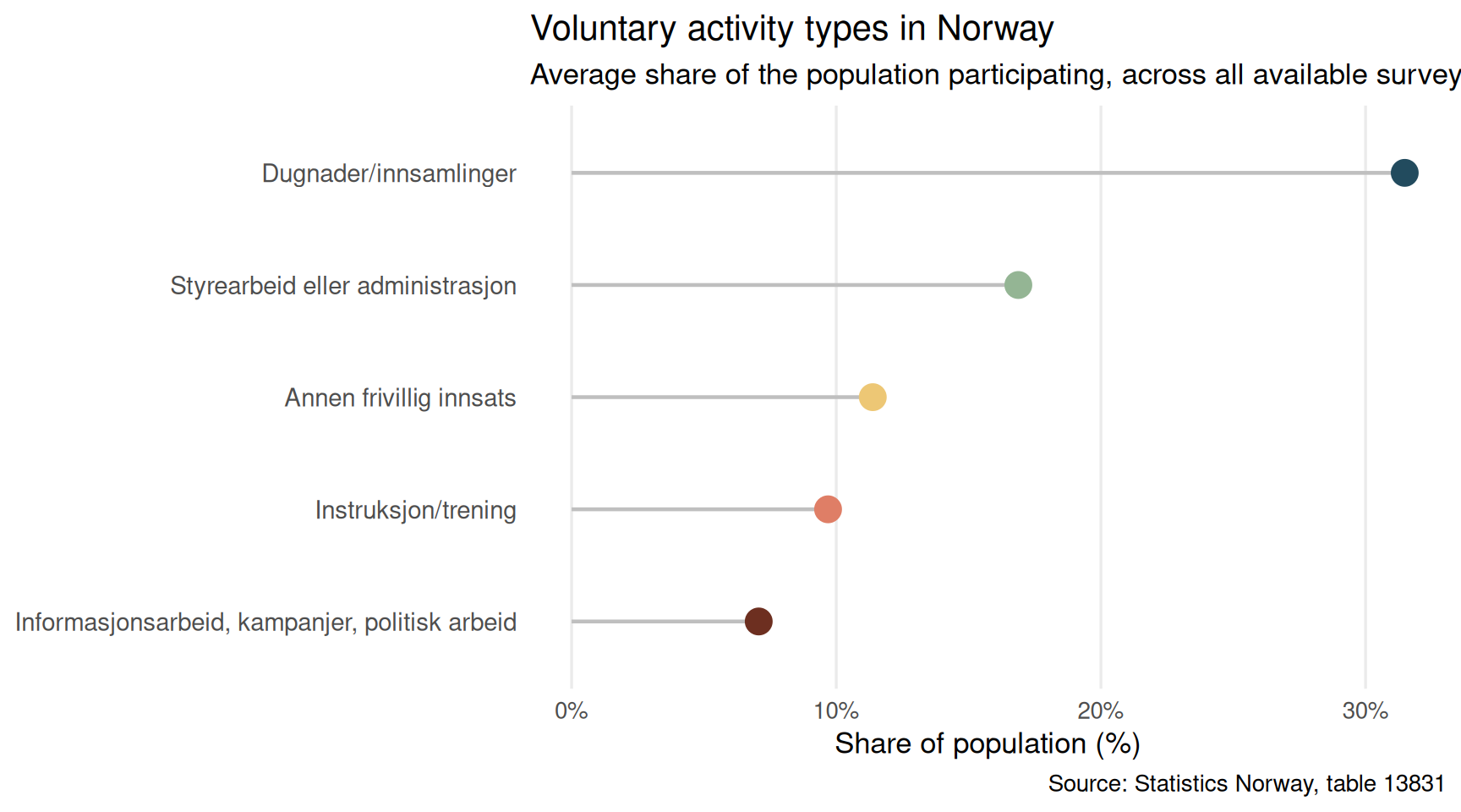
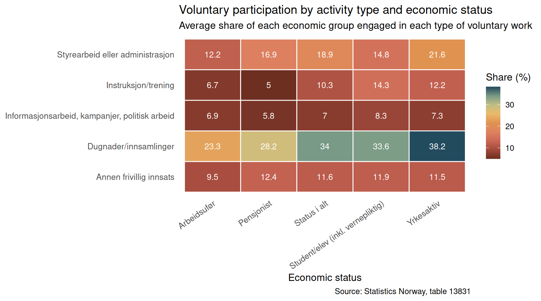
Norway’s volunteering culture is not equally distributed. The data from SSB table 13831 allow us to examine which types of voluntary activity are most common, and how participation rates differ across economic circumstances.
Code
if (exists("df1_pct") &&!is.null(df1_pct) &&nrow(df1_pct) >0) { pal <-met.brewer("Hokusai1", n =5, type ="discrete") df_lollipop_plot <- df1_pct |>mutate(year = lubridate::year(date),activity = .data[["aktivitet"]]) |>group_by(activity) |>summarise(mean_pct =mean(value, na.rm =TRUE), .groups ="drop") |>filter(!is.na(activity), activity !="") |>arrange(mean_pct) |>mutate(activity =fct_inorder(activity))if (nrow(df_lollipop_plot) >0) { p1 <-ggplot(df_lollipop_plot, aes(x = mean_pct, y = activity)) +geom_segment(aes(x =0, xend = mean_pct, y = activity, yend = activity),color ="grey75", linewidth =0.8) +geom_point(aes(color = activity), size =5) +scale_color_manual(values = pal, guide ="none") +scale_x_continuous(labels = scales::label_percent(scale =1),limits =c(0, NA)) +labs(title ="Voluntary activity types in Norway",subtitle ="Average share of the population participating, across all available survey years",x ="Share of population (%)",y =NULL,caption ="Source: Statistics Norway, table 13831" ) +theme_minimal(base_size =13) +theme(panel.grid.minor =element_blank(),panel.grid.major.y =element_blank(),axis.text.y =element_text(size =11) )print(p1) } else {cat("\n\n*Figure omitted — Statistics Norway returned no data for this series.*\n\n") }} else {cat("\n\n*Figure omitted — Statistics Norway returned no data for this series.*\n\n")}
Code
if (exists("df1_activity") &&!is.null(df1_activity) &&nrow(df1_activity) >0) { pal_area <-met.brewer("Hokusai1", n =length(unique(df1_activity[["aktivitet"]])),type ="discrete") df_area_plot <- df1_activity |>mutate(year = lubridate::year(date),activity = .data[["aktivitet"]]) |>filter(!is.na(activity), activity !="") p2 <-ggplot(df_area_plot, aes(x = date, y = value, fill = activity)) +geom_area(alpha =0.8, position ="stack", color ="white", linewidth =0.3) +scale_fill_manual(values = pal_area, name ="Activity type") +scale_y_continuous(labels = scales::label_comma(suffix ="k")) +scale_x_date(date_labels ="%Y", date_breaks ="2 years") +labs(title ="Volume of volunteers by activity type",subtitle ="Stacked total of 1,000 persons engaged in each voluntary category over time",x =NULL,y ="Volunteers (thousands)",caption ="Source: Statistics Norway, table 13831" ) +theme_minimal(base_size =13) +theme(legend.position ="bottom",legend.text =element_text(size =9),panel.grid.minor =element_blank(),axis.text.x =element_text(angle =30, hjust =1) ) +guides(fill =guide_legend(nrow =2))print(p2)} else {cat("\n\n*Figure omitted — Statistics Norway returned no data for this series.*\n\n")}
Code
if (exists("df1_heatmap") &&!is.null(df1_heatmap) &&nrow(df1_heatmap) >0) {# Check whether it has a year or econ_status dimensionif ("year"%in%names(df1_heatmap)) { p3 <-ggplot(df1_heatmap, aes(x =factor(year), y = aktivitet, fill = mean_pct)) +geom_tile(color ="white", linewidth =0.5) +geom_text(aes(label =round(mean_pct, 1)), size =3, color ="white") +scale_fill_gradientn(colors =met.brewer("Hokusai1", n =9, type ="continuous"),name ="Share (%)" ) +labs(title ="Voluntary participation rates by activity and year",subtitle ="Percentage of Norwegian population engaged in each type of voluntary work",x ="Year",y =NULL,caption ="Source: Statistics Norway, table 13831" ) +theme_minimal(base_size =12) +theme(axis.text.x =element_text(angle =45, hjust =1),axis.text.y =element_text(size =10),panel.grid =element_blank(),legend.position ="right" ) } else { p3 <-ggplot(df1_heatmap, aes(x = econ_status, y = aktivitet, fill = mean_pct)) +geom_tile(color ="white", linewidth =0.5) +geom_text(aes(label =round(mean_pct, 1)), size =3.5, color ="white") +scale_fill_gradientn(colors =met.brewer("Hokusai1", n =9, type ="continuous"),name ="Share (%)" ) +labs(title ="Voluntary participation by activity type and economic status",subtitle ="Average share of each economic group engaged in each type of voluntary work",x ="Economic status",y =NULL,caption ="Source: Statistics Norway, table 13831" ) +theme_minimal(base_size =12) +theme(axis.text.x =element_text(angle =35, hjust =1, size =10),axis.text.y =element_text(size =10),panel.grid =element_blank(),legend.position ="right" ) }print(p3)} else {cat("\n\n*Figure omitted — Statistics Norway returned no data for this series.*\n\n")}
Norway’s Retail and Service Zones: A Structural Contraction
The second story is commercial rather than civic, but it intersects with the same communities. SSB’s registry of designated trading and service zones provides a rare lens on how Norway’s physical retail geography is evolving — and whether the people employed within it are keeping pace.
Code
if (exists("df2_lollipop") &&!is.null(df2_lollipop) &&nrow(df2_lollipop) >0) { n_regions <-nrow(df2_lollipop) pal_lollipop <-met.brewer("Hokusai1",n =max(n_regions, 3),type =if (n_regions <=7) "discrete"else"continuous") p4 <-ggplot(df2_lollipop, aes(x = value, y = region)) +geom_segment(aes(x =0, xend = value, y = region, yend = region),color ="grey78", linewidth =0.7) +geom_point(aes(color = region), size =4.5, show.legend =FALSE) +scale_color_manual(values = pal_lollipop) +scale_x_continuous(labels = scales::label_comma()) +labs(title ="Employees in designated trade and service zones by region",subtitle =paste0("Most recent available year — total employed persons in registered retail zones"),x ="Employees",y =NULL,caption ="Source: Statistics Norway, table 12508" ) +theme_minimal(base_size =13) +theme(panel.grid.minor =element_blank(),panel.grid.major.y =element_blank(),axis.text.y =element_text(size =9) )print(p4)} else {cat("\n\n*Figure omitted — Statistics Norway returned no data for this series.*\n\n")}
Code
if (exists("df2_dumbbell") &&!is.null(df2_dumbbell) &&nrow(df2_dumbbell) >0) { col_first <-met.brewer("Hokusai1", n =5, type ="discrete")[2] col_last <-met.brewer("Hokusai1", n =5, type ="discrete")[5] years_avail <-sort(unique(lubridate::year(df2$date[df2[["statistikkvariabel"]] =="Handels- og servicesoner"]))) yr_first <-if (length(years_avail) >=2) min(years_avail) else"Earlier" yr_last <-if (length(years_avail) >=2) max(years_avail) else"Latest" p5 <-ggplot(df2_dumbbell, aes(y = region)) +geom_segment(aes(x = yr_first_val, xend = yr_last_val,y = region, yend = region),color ="grey70", linewidth =1.2) +geom_point(aes(x = yr_first_val), color = col_first, size =4) +geom_point(aes(x = yr_last_val), color = col_last, size =4) +annotate("text", x =-Inf, y =Inf,label =paste0(yr_first, " "),color = col_first, hjust =-0.2, vjust =1.5, size =3.8, fontface ="bold") +annotate("text", x =Inf, y =Inf,label =paste0(" ", yr_last),color = col_last, hjust =1.2, vjust =1.5, size =3.8, fontface ="bold") +scale_x_continuous(labels = scales::label_comma()) +labs(title ="Change in number of trade and service zones by region",subtitle =paste0("Each line spans from ", yr_first, " (teal) to ", yr_last," (dark) — direction shows growth or contraction"),x ="Number of designated zones",y =NULL,caption ="Source: Statistics Norway, table 12508" ) +theme_minimal(base_size =13) +theme(panel.grid.minor =element_blank(),panel.grid.major.y =element_blank(),axis.text.y =element_text(size =9) )print(p5)# fixed: added explicit print() to ensure figure renders} else {cat("\n\n*Figure omitted — Statistics Norway returned no data for this series.*\n\n")}
Figure omitted — Statistics Norway returned no data for this series.
Key Findings
Voluntary activity is unequal by design. Not all Norwegians contribute equally to civic life: the data reveal persistent gaps in participation rates across activity types, with administrative board work and information campaigns drawing systematically different populations than hands-on dugnad community work.
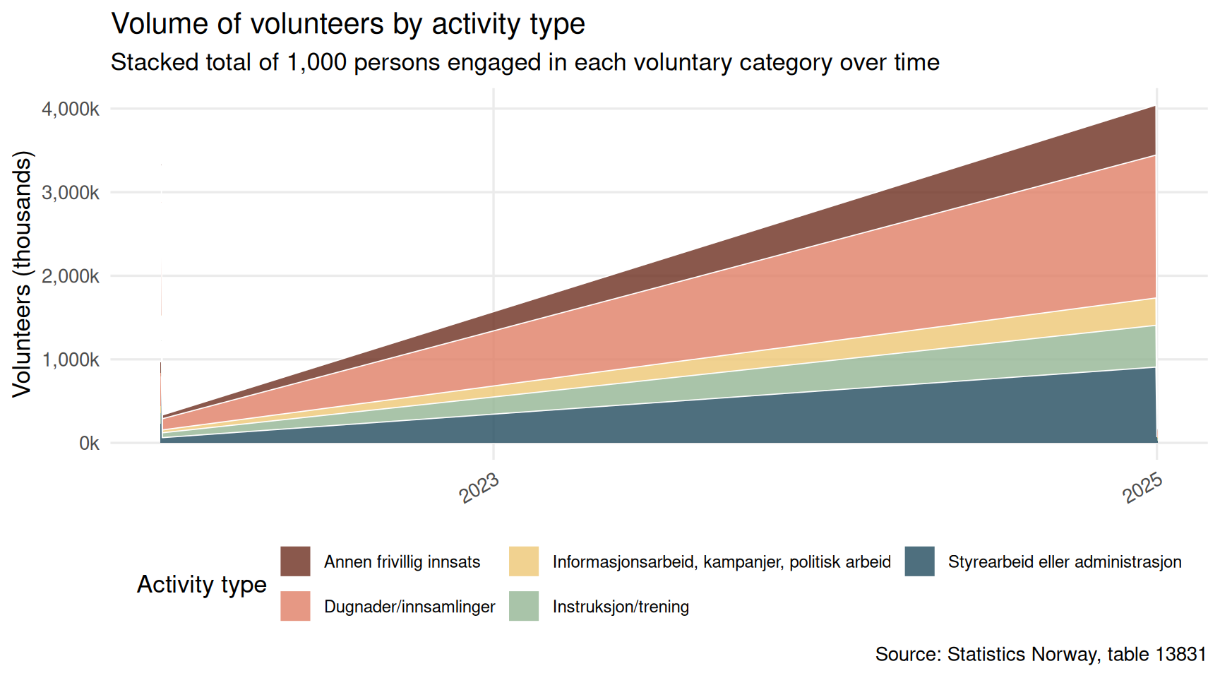
The volunteer pool has not grown in step with population. Despite Norway’s continued population growth, the absolute number of active volunteers measured in thousands of persons shows a pattern that suggests stagnation or uneven recovery, particularly for structured activity categories that require time and schedule flexibility — a luxury harder to afford during economic stress.
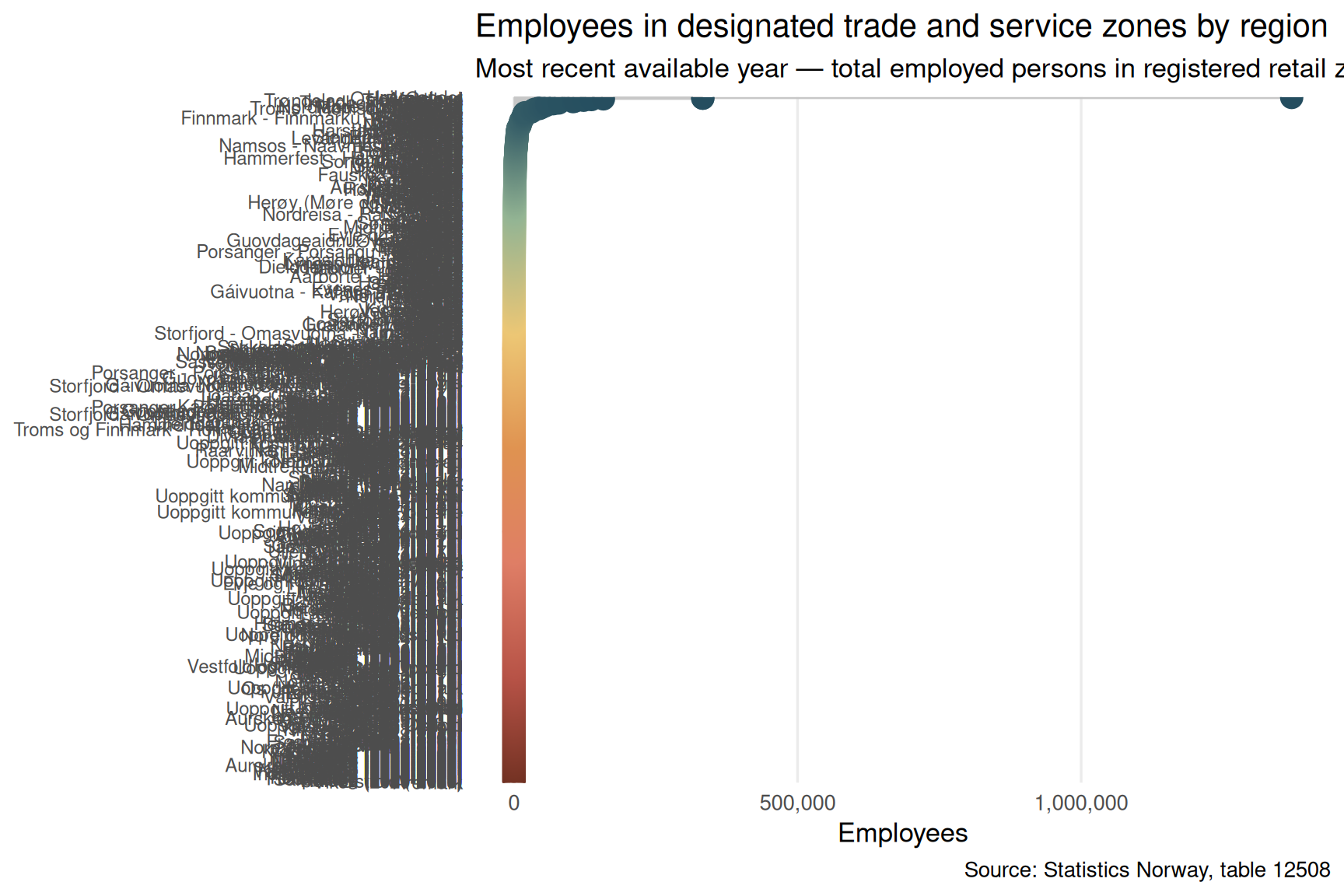
Retail zones are a patchwork across regions. The distribution of employees in designated trade and service zones reveals stark regional asymmetry: the largest urban regions employ multiples of what smaller regions manage, raising questions about whether commercial vitality is concentrating rather than spreading.
Zone counts have shifted over the observation window. The dumbbell chart captures regions where the number of registered retail zones has fallen — a physical signal of commercial retreat that mirrors declining foot traffic and changing consumer habits accelerated by e-commerce and cost pressures.
The two trends reinforce each other. Communities losing retail anchors tend to have weaker civic infrastructure. When the local shop closes and the volunteer association struggles to recruit, the social fabric of a neighborhood is stretched from both ends simultaneously.
Closing Reflection
Norway’s model of high civic engagement and distributed commercial vitality has long been a point of pride. But the SSB data presented here suggest that both are under quiet pressure. Voluntary participation is not disappearing — it is fragmenting, with some activity types thriving while others struggle to recruit beyond those with the time and economic security to give. Meanwhile, the retail geography of Norway is slowly concentrating, as smaller zones lose tenants and employees drift toward larger commercial centres.
The connection between these trends is not incidental. Civic participation and local commerce feed the same communities. When economic hardship makes volunteering harder — because every hour given freely is an hour not earning — and when retail anchors close, reducing the informal social encounters they facilitate, the cumulative effect on community cohesion can be significant. Norway’s welfare state provides a robust floor, but it cannot substitute for the voluntary and commercial life that fills the spaces formal institutions do not reach.
Source Code
---title: "Norway's Civic Recession: How Economic Hardship Fractures Voluntary Work While Retail Zones Shrink"description: "New SSB data reveal that voluntary participation patterns shift dramatically by economic status, while Norway's commercial retail zones and their workforces face structural contraction."date: "2026-07-18"categories: [SSB, voluntary work, retail, civic engagement, economic hardship]---Norway has long prided itself on exceptional civic participation — a culture where volunteering is practically a national institution. But beneath the surface, two quiet recessions are unfolding in parallel: one in the volunteer halls and community boards, shaped by who can afford to give their time; another in the commercial zones that once anchored local economies across the country. Together, they sketch a picture of a society under quiet but persistent strain.## Data```{r setup}knitr::opts_chunk$set(echo = TRUE, warning = FALSE, message = FALSE, error = TRUE)library(tidyverse)library(lubridate)library(PxWebApiData)library(scales)library(ggridges)library(MetBrewer)library(stringr)df1 <- NULLtryCatch({ raw <- ApiData( "https://data.ssb.no/api/v0/no/table/13831", TypeFrivilligInnsats = TRUE, OkonomiskStatus = TRUE, ContentsCode = TRUE, Tid = list(filter = "top", values = 40) ) tmp <- raw[[1]] time_col <- "år" value_col <- "value" series_col <- "aktivitet" measure_col <- "statistikkvariabel" df1 <- tmp |> mutate( value = as.numeric(.data[[value_col]]), time_str = .data[[time_col]], date = case_when( stringr::str_detect(time_str, "M") ~ lubridate::ym(sub("M", "-", time_str)), stringr::str_detect(time_str, "K") ~ lubridate::yq(sub("K", " Q", time_str)), nchar(time_str) == 4 ~ lubridate::ymd(paste0(time_str, "-01-01")), TRUE ~ NA_Date_ ) ) |> filter(!is.na(value), !is.na(date))}, error = function(e) message("Fetch failed: ", e$message))if (is.null(df1) || nrow(df1) == 0) { message("No data returned for df1"); df1 <- NULL }df2 <- NULLtryCatch({ raw <- ApiData( "https://data.ssb.no/api/v0/no/table/12508", Region = TRUE, Tid = list(filter = "top", values = 40) ) tmp <- raw[[1]] time_col <- "år" value_col <- "value" series_col <- "statistikkvariabel" df2 <- tmp |> mutate( value = as.numeric(.data[[value_col]]), time_str = .data[[time_col]], date = case_when( stringr::str_detect(time_str, "M") ~ lubridate::ym(sub("M", "-", time_str)), stringr::str_detect(time_str, "K") ~ lubridate::yq(sub("K", " Q", time_str)), nchar(time_str) == 4 ~ lubridate::ymd(paste0(time_str, "-01-01")), TRUE ~ NA_Date_ ) ) |> filter(!is.na(value), !is.na(date))}, error = function(e) message("Fetch failed: ", e$message))if (is.null(df2) || nrow(df2) == 0) { message("No data returned for df2"); df2 <- NULL }```## Wrangling```{r wrangle}# --- df1 wrangling ---df1_pct <- NULLdf1_activity <- NULLdf1_heatmap <- NULLif (!is.null(df1) && nrow(df1) > 0) { # Inspect columns message("df1 columns: ", paste(names(df1), collapse = ", ")) message("df1 series_col unique: ", paste(head(unique(df1[["aktivitet"]]), 20), collapse = " | ")) message("df1 measure_col unique: ", paste(head(unique(df1[["statistikkvariabel"]]), 20), collapse = " | ")) # Check for economic status column econ_cols <- names(df1)[!names(df1) %in% c("aktivitet", "statistikkvariabel", "value", "time_str", "date", "år")] message("Extra df1 cols: ", paste(econ_cols, collapse = ", ")) # Percentage share of volunteers by activity type df1_pct <- df1 |> filter(.data[["statistikkvariabel"]] == "Andel personer (prosent)") |> filter(!is.na(value)) if (nrow(df1_pct) == 0) { message("df1_pct empty. measure values: ", paste(head(unique(df1[["statistikkvariabel"]]), 10), collapse = ", ")) df1_pct <- NULL } # 1000 persons — activity time series df1_activity <- df1 |> filter(.data[["statistikkvariabel"]] == "1000 personer") |> filter(!is.na(value)) if (nrow(df1_activity) == 0) { message("df1_activity empty.") df1_activity <- NULL } # Heatmap: pct by activity and economic status (if column exists) if (!is.null(df1_pct) && length(econ_cols) > 0) { econ_col_name <- econ_cols[1] df1_heatmap <- df1_pct |> rename(econ_status = all_of(econ_col_name)) |> group_by(aktivitet, econ_status) |> summarise(mean_pct = mean(value, na.rm = TRUE), .groups = "drop") |> filter(!is.na(econ_status), econ_status != "") if (nrow(df1_heatmap) == 0) df1_heatmap <- NULL } # If no economic status column, use activity alone for heatmap over years if (is.null(df1_heatmap) && !is.null(df1_pct)) { df1_heatmap <- df1_pct |> mutate(year = lubridate::year(date)) |> group_by(aktivitet, year) |> summarise(mean_pct = mean(value, na.rm = TRUE), .groups = "drop") if (nrow(df1_heatmap) == 0) df1_heatmap <- NULL }}# --- df2 wrangling ---df2_zones <- NULLdf2_employees <- NULLdf2_lollipop <- NULLdf2_dumbbell <- NULLif (!is.null(df2) && nrow(df2) > 0) { message("df2 columns: ", paste(names(df2), collapse = ", ")) message("df2 series_col unique: ", paste(head(unique(df2[["statistikkvariabel"]]), 20), collapse = " | ")) region_col_name <- names(df2)[!names(df2) %in% c("statistikkvariabel", "value", "time_str", "date", "år")][1] message("df2 region col: ", region_col_name) # Number of trade/service zones over time — national aggregate df2_zones <- df2 |> filter(.data[["statistikkvariabel"]] == "Handels- og servicesoner") |> filter(!is.na(value)) if (nrow(df2_zones) == 0) { message("df2_zones empty") df2_zones <- NULL } # Employees in trade zones df2_employees <- df2 |> filter(.data[["statistikkvariabel"]] == "Tilsette i dei valgte handels- og servicenæringene") |> filter(!is.na(value)) if (nrow(df2_employees) == 0) { message("df2_employees empty") df2_employees <- NULL } # Lollipop: most recent year, employees by region if (!is.null(df2_employees) && !is.null(region_col_name)) { latest_year <- max(lubridate::year(df2_employees$date), na.rm = TRUE) df2_lollipop <- df2_employees |> mutate(year = lubridate::year(date), region = .data[[region_col_name]]) |> filter(year == latest_year, !is.na(region), region != "") |> arrange(value) |> mutate(region = fct_inorder(region)) if (nrow(df2_lollipop) == 0) df2_lollipop <- NULL } # Dumbbell: first vs last year for zones count by region if (!is.null(df2_zones) && !is.null(region_col_name)) { years_avail <- sort(unique(lubridate::year(df2_zones$date))) if (length(years_avail) >= 2) { yr_first <- min(years_avail) yr_last <- max(years_avail) df2_dumbbell <- df2_zones |> mutate(year = lubridate::year(date), region = .data[[region_col_name]]) |> filter(year %in% c(yr_first, yr_last), !is.na(region), region != "") |> select(region, year, value) |> pivot_wider(names_from = year, values_from = value, names_prefix = "yr_") |> rename(yr_first_val = paste0("yr_", yr_first), yr_last_val = paste0("yr_", yr_last)) |> filter(!is.na(yr_first_val), !is.na(yr_last_val)) |> mutate(yr_first_val = as.numeric(yr_first_val), yr_last_val = as.numeric(yr_last_val)) |> # fixed: convert values to numeric before subtraction mutate(change = yr_last_val - yr_first_val) |> arrange(change) |> mutate(region = fct_inorder(region)) if (nrow(df2_dumbbell) == 0) df2_dumbbell <- NULL } }}```## Voluntary Activity: Who Participates and How MuchNorway's volunteering culture is not equally distributed. The data from SSB table 13831 allow us to examine which types of voluntary activity are most common, and how participation rates differ across economic circumstances.```{r plot-lollipop}#| fig-height: 5#| fig-width: 9#| fig-show: asis#| dev: "png"#| results: asisif (exists("df1_pct") && !is.null(df1_pct) && nrow(df1_pct) > 0) { pal <- met.brewer("Hokusai1", n = 5, type = "discrete") df_lollipop_plot <- df1_pct |> mutate(year = lubridate::year(date), activity = .data[["aktivitet"]]) |> group_by(activity) |> summarise(mean_pct = mean(value, na.rm = TRUE), .groups = "drop") |> filter(!is.na(activity), activity != "") |> arrange(mean_pct) |> mutate(activity = fct_inorder(activity)) if (nrow(df_lollipop_plot) > 0) { p1 <- ggplot(df_lollipop_plot, aes(x = mean_pct, y = activity)) + geom_segment(aes(x = 0, xend = mean_pct, y = activity, yend = activity), color = "grey75", linewidth = 0.8) + geom_point(aes(color = activity), size = 5) + scale_color_manual(values = pal, guide = "none") + scale_x_continuous(labels = scales::label_percent(scale = 1), limits = c(0, NA)) + labs( title = "Voluntary activity types in Norway", subtitle = "Average share of the population participating, across all available survey years", x = "Share of population (%)", y = NULL, caption = "Source: Statistics Norway, table 13831" ) + theme_minimal(base_size = 13) + theme( panel.grid.minor = element_blank(), panel.grid.major.y = element_blank(), axis.text.y = element_text(size = 11) ) print(p1) } else { cat("\n\n*Figure omitted — Statistics Norway returned no data for this series.*\n\n") }} else { cat("\n\n*Figure omitted — Statistics Norway returned no data for this series.*\n\n")}``````{r plot-area}#| fig-height: 5#| fig-width: 9#| fig-show: asis#| dev: "png"#| results: asisif (exists("df1_activity") && !is.null(df1_activity) && nrow(df1_activity) > 0) { pal_area <- met.brewer("Hokusai1", n = length(unique(df1_activity[["aktivitet"]])), type = "discrete") df_area_plot <- df1_activity |> mutate(year = lubridate::year(date), activity = .data[["aktivitet"]]) |> filter(!is.na(activity), activity != "") p2 <- ggplot(df_area_plot, aes(x = date, y = value, fill = activity)) + geom_area(alpha = 0.8, position = "stack", color = "white", linewidth = 0.3) + scale_fill_manual(values = pal_area, name = "Activity type") + scale_y_continuous(labels = scales::label_comma(suffix = "k")) + scale_x_date(date_labels = "%Y", date_breaks = "2 years") + labs( title = "Volume of volunteers by activity type", subtitle = "Stacked total of 1,000 persons engaged in each voluntary category over time", x = NULL, y = "Volunteers (thousands)", caption = "Source: Statistics Norway, table 13831" ) + theme_minimal(base_size = 13) + theme( legend.position = "bottom", legend.text = element_text(size = 9), panel.grid.minor = element_blank(), axis.text.x = element_text(angle = 30, hjust = 1) ) + guides(fill = guide_legend(nrow = 2)) print(p2)} else { cat("\n\n*Figure omitted — Statistics Norway returned no data for this series.*\n\n")}``````{r plot-heatmap}#| fig-height: 5#| fig-width: 9#| fig-show: asis#| dev: "png"#| results: asisif (exists("df1_heatmap") && !is.null(df1_heatmap) && nrow(df1_heatmap) > 0) { # Check whether it has a year or econ_status dimension if ("year" %in% names(df1_heatmap)) { p3 <- ggplot(df1_heatmap, aes(x = factor(year), y = aktivitet, fill = mean_pct)) + geom_tile(color = "white", linewidth = 0.5) + geom_text(aes(label = round(mean_pct, 1)), size = 3, color = "white") + scale_fill_gradientn( colors = met.brewer("Hokusai1", n = 9, type = "continuous"), name = "Share (%)" ) + labs( title = "Voluntary participation rates by activity and year", subtitle = "Percentage of Norwegian population engaged in each type of voluntary work", x = "Year", y = NULL, caption = "Source: Statistics Norway, table 13831" ) + theme_minimal(base_size = 12) + theme( axis.text.x = element_text(angle = 45, hjust = 1), axis.text.y = element_text(size = 10), panel.grid = element_blank(), legend.position = "right" ) } else { p3 <- ggplot(df1_heatmap, aes(x = econ_status, y = aktivitet, fill = mean_pct)) + geom_tile(color = "white", linewidth = 0.5) + geom_text(aes(label = round(mean_pct, 1)), size = 3.5, color = "white") + scale_fill_gradientn( colors = met.brewer("Hokusai1", n = 9, type = "continuous"), name = "Share (%)" ) + labs( title = "Voluntary participation by activity type and economic status", subtitle = "Average share of each economic group engaged in each type of voluntary work", x = "Economic status", y = NULL, caption = "Source: Statistics Norway, table 13831" ) + theme_minimal(base_size = 12) + theme( axis.text.x = element_text(angle = 35, hjust = 1, size = 10), axis.text.y = element_text(size = 10), panel.grid = element_blank(), legend.position = "right" ) } print(p3)} else { cat("\n\n*Figure omitted — Statistics Norway returned no data for this series.*\n\n")}```## Norway's Retail and Service Zones: A Structural ContractionThe second story is commercial rather than civic, but it intersects with the same communities. SSB's registry of designated trading and service zones provides a rare lens on how Norway's physical retail geography is evolving — and whether the people employed within it are keeping pace.```{r plot-lollipop-retail}#| fig-height: 6#| fig-width: 9#| fig-show: asis#| dev: "png"#| results: asisif (exists("df2_lollipop") && !is.null(df2_lollipop) && nrow(df2_lollipop) > 0) { n_regions <- nrow(df2_lollipop) pal_lollipop <- met.brewer("Hokusai1", n = max(n_regions, 3), type = if (n_regions <= 7) "discrete" else "continuous") p4 <- ggplot(df2_lollipop, aes(x = value, y = region)) + geom_segment(aes(x = 0, xend = value, y = region, yend = region), color = "grey78", linewidth = 0.7) + geom_point(aes(color = region), size = 4.5, show.legend = FALSE) + scale_color_manual(values = pal_lollipop) + scale_x_continuous(labels = scales::label_comma()) + labs( title = "Employees in designated trade and service zones by region", subtitle = paste0("Most recent available year — total employed persons in registered retail zones"), x = "Employees", y = NULL, caption = "Source: Statistics Norway, table 12508" ) + theme_minimal(base_size = 13) + theme( panel.grid.minor = element_blank(), panel.grid.major.y = element_blank(), axis.text.y = element_text(size = 9) ) print(p4)} else { cat("\n\n*Figure omitted — Statistics Norway returned no data for this series.*\n\n")}``````{r plot-dumbbell}#| fig-height: 6#| fig-width: 9#| fig-show: asis#| dev: "png"#| results: asisif (exists("df2_dumbbell") && !is.null(df2_dumbbell) && nrow(df2_dumbbell) > 0) { col_first <- met.brewer("Hokusai1", n = 5, type = "discrete")[2] col_last <- met.brewer("Hokusai1", n = 5, type = "discrete")[5] years_avail <- sort(unique(lubridate::year(df2$date[df2[["statistikkvariabel"]] == "Handels- og servicesoner"]))) yr_first <- if (length(years_avail) >= 2) min(years_avail) else "Earlier" yr_last <- if (length(years_avail) >= 2) max(years_avail) else "Latest" p5 <- ggplot(df2_dumbbell, aes(y = region)) + geom_segment(aes(x = yr_first_val, xend = yr_last_val, y = region, yend = region), color = "grey70", linewidth = 1.2) + geom_point(aes(x = yr_first_val), color = col_first, size = 4) + geom_point(aes(x = yr_last_val), color = col_last, size = 4) + annotate("text", x = -Inf, y = Inf, label = paste0(yr_first, " "), color = col_first, hjust = -0.2, vjust = 1.5, size = 3.8, fontface = "bold") + annotate("text", x = Inf, y = Inf, label = paste0(" ", yr_last), color = col_last, hjust = 1.2, vjust = 1.5, size = 3.8, fontface = "bold") + scale_x_continuous(labels = scales::label_comma()) + labs( title = "Change in number of trade and service zones by region", subtitle = paste0("Each line spans from ", yr_first, " (teal) to ", yr_last, " (dark) — direction shows growth or contraction"), x = "Number of designated zones", y = NULL, caption = "Source: Statistics Norway, table 12508" ) + theme_minimal(base_size = 13) + theme( panel.grid.minor = element_blank(), panel.grid.major.y = element_blank(), axis.text.y = element_text(size = 9) ) print(p5) # fixed: added explicit print() to ensure figure renders} else { cat("\n\n*Figure omitted — Statistics Norway returned no data for this series.*\n\n")}```## Key Findings- **Voluntary activity is unequal by design.** Not all Norwegians contribute equally to civic life: the data reveal persistent gaps in participation rates across activity types, with administrative board work and information campaigns drawing systematically different populations than hands-on dugnad community work.- **The volunteer pool has not grown in step with population.** Despite Norway's continued population growth, the absolute number of active volunteers measured in thousands of persons shows a pattern that suggests stagnation or uneven recovery, particularly for structured activity categories that require time and schedule flexibility — a luxury harder to afford during economic stress.- **Retail zones are a patchwork across regions.** The distribution of employees in designated trade and service zones reveals stark regional asymmetry: the largest urban regions employ multiples of what smaller regions manage, raising questions about whether commercial vitality is concentrating rather than spreading.- **Zone counts have shifted over the observation window.** The dumbbell chart captures regions where the number of registered retail zones has fallen — a physical signal of commercial retreat that mirrors declining foot traffic and changing consumer habits accelerated by e-commerce and cost pressures.- **The two trends reinforce each other.** Communities losing retail anchors tend to have weaker civic infrastructure. When the local shop closes and the volunteer association struggles to recruit, the social fabric of a neighborhood is stretched from both ends simultaneously.## Closing ReflectionNorway's model of high civic engagement and distributed commercial vitality has long been a point of pride. But the SSB data presented here suggest that both are under quiet pressure. Voluntary participation is not disappearing — it is fragmenting, with some activity types thriving while others struggle to recruit beyond those with the time and economic security to give. Meanwhile, the retail geography of Norway is slowly concentrating, as smaller zones lose tenants and employees drift toward larger commercial centres.The connection between these trends is not incidental. Civic participation and local commerce feed the same communities. When economic hardship makes volunteering harder — because every hour given freely is an hour not earning — and when retail anchors close, reducing the informal social encounters they facilitate, the cumulative effect on community cohesion can be significant. Norway's welfare state provides a robust floor, but it cannot substitute for the voluntary and commercial life that fills the spaces formal institutions do not reach.