A data-driven examination of how Norway’s greenhouse gas emissions by sector reveal a widening gap between climate ambitions and the fossil fuel reality underpinning the national economy.
Published
July 17, 2026
Norway presents one of the most striking contradictions in global climate politics: a nation that leads the world in electric vehicle adoption, generates nearly all its electricity from hydropower, and has pledged to cut emissions by 55 percent by 2030 — yet remains one of the world’s largest per capita exporters of oil and gas. The numbers from Statistics Norway tell a story of structural inertia, where ambitious green rhetoric collides with the stubborn weight of extraction-driven emissions.
# Initialise all derived data frames to NULL before any conditional logicdf_co2eq <-NULLdf_sectors <-NULLdf_total <-NULLdf_wide <-NULLdf_slope <-NULLdf_heat <-NULLdf_lollipop <-NULLdf_change <-NULLif (!is.null(df) &&nrow(df) >0) {# Filter for CO2-equivalent measure — the standard policy metric df_co2eq <- df |>filter(.data[[measure_col]] =="Utslipp til luft (1 000 tonn CO2-ekvivalenter, AR5)")# Sector-level breakdown — all sources including "Alle kilder" (total) df_sectors <- df_co2eq |>rename(source =all_of(series_col),year = date ) |>mutate(year_int = lubridate::year(year))# Total emissions only df_total <- df_sectors |>filter(source =="Alle kilder")# Sector breakdown excluding total df_sectors_sub <- df_sectors |>filter(source !="Alle kilder")# Year range available yr_min <-min(df_sectors$year_int, na.rm =TRUE) yr_max <-max(df_sectors$year_int, na.rm =TRUE)# For lollipop: latest year change vs earliest for each sector df_lollipop <- df_sectors_sub |>filter(year_int %in%c(yr_min, yr_max)) |>select(source, year_int, value) |>pivot_wider(names_from = year_int, values_from = value) |>rename(val_start =2, val_end =3) |>mutate(val_start =as.numeric(val_start), # fixed: coerce to numeric after pivot_widerval_end =as.numeric(val_end), # fixed: coerce to numeric after pivot_widerchange_abs = val_end - val_start,change_pct = (val_end - val_start) / val_start *100,direction =if_else(change_abs <0, "Decrease", "Increase") ) |>filter(!is.na(change_abs)) |>arrange(change_pct)# For heatmap: all years × all sectors (excl total) df_heat <- df_sectors_sub |>select(source, year_int, value) |>group_by(source) |>mutate(index = value /first(value) *100# index to first available year ) |>ungroup()# For slope chart: first and last year per sector (excl total) df_slope <- df_sectors_sub |>filter(year_int %in%c(yr_min, yr_max)) |>select(source, year_int, value)# Sector share in latest year total_latest <- df_total |>filter(year_int == yr_max) |>pull(value) df_share <- df_sectors_sub |>filter(year_int == yr_max) |>mutate(share = value / total_latest *100) |>arrange(desc(share))message("Years available: ", yr_min, " to ", yr_max)message("Total emissions (latest year): ", total_latest, " thousand tonnes CO2eq")message("Sectors: ", paste(unique(df_sectors_sub$source), collapse ="; "))}
Error in `mutate()`:
ℹ In argument: `val_start = as.numeric(val_start)`.
Caused by error:
! 'list' object cannot be coerced to type 'double'
The Total Trajectory: Norway’s Emissions Over Time
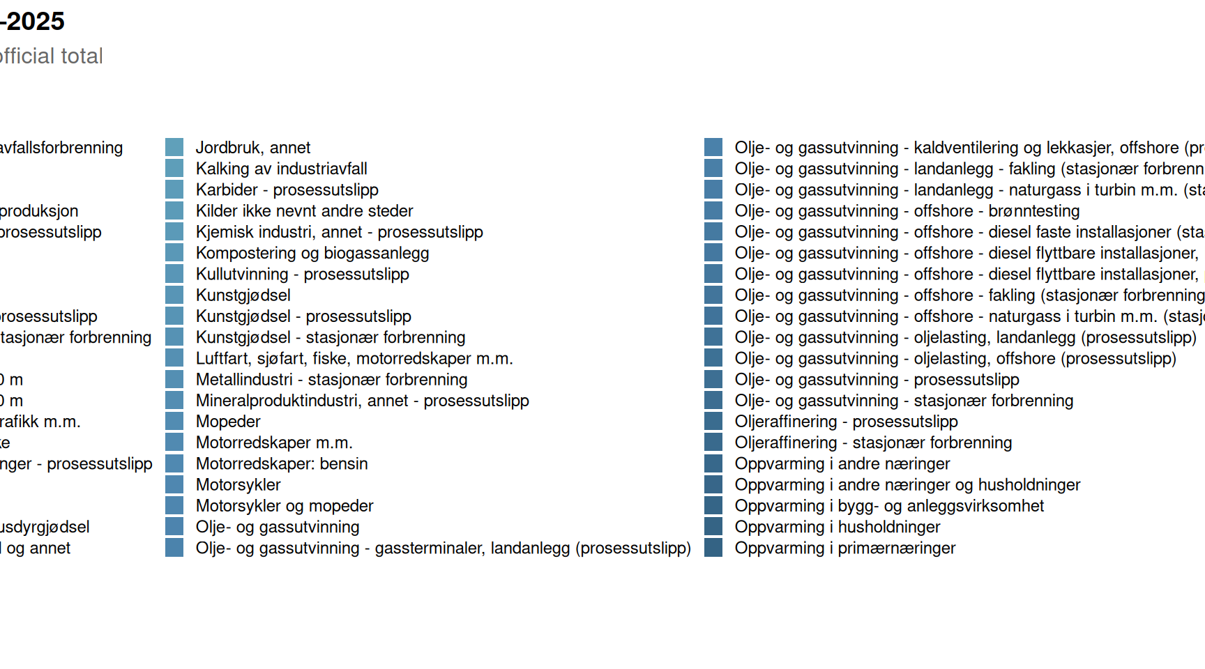
Norway has long pointed to its per-household renewable electricity system as evidence of climate leadership. But total greenhouse gas emissions, measured in CO2 equivalents, tell a more complicated story — one shaped overwhelmingly by what happens offshore and in heavy industry onshore.
Code
if (exists("df_total") &&!is.null(df_total) &&nrow(df_total) >0&&exists("df_sectors") &&!is.null(df_sectors) &&nrow(df_sectors) >0) {# Use sector breakdown for stacked area, total as overlay line df_sectors_sub_plot <- df_sectors |>filter(source !="Alle kilder") sector_palette <-met.brewer("Hokusai2", n =length(unique(df_sectors_sub_plot$source))) p1 <-ggplot() +geom_area(data = df_sectors_sub_plot,aes(x = year, y = value, fill = source),alpha =0.85,position ="stack" ) +geom_line(data = df_total,aes(x = year, y = value),colour ="grey20",linewidth =0.8,linetype ="dashed" ) +scale_fill_manual(values = sector_palette) +scale_y_continuous(labels =label_comma(suffix ="k t"),expand =expansion(mult =c(0, 0.05)) ) +scale_x_date(date_breaks ="1 year", date_labels ="%Y") +labs(title ="Norway's greenhouse gas emissions by sector, 2021–2025",subtitle ="Oil and gas extraction consistently dominates; dashed line shows official total",x =NULL,y ="1 000 tonnes CO\u2082-equivalents (AR5)",fill ="Emission source",caption ="Source: Statistics Norway, table 13931" ) +theme_minimal(base_size =12) +theme(plot.title =element_text(face ="bold", size =14),plot.subtitle =element_text(colour ="grey40", margin =margin(b =8)),legend.position ="right",legend.key.size =unit(0.4, "cm"),legend.text =element_text(size =9),axis.text.x =element_text(angle =45, hjust =1),panel.grid.minor =element_blank() )print(p1)} else {cat("\n\n*Figure omitted — Statistics Norway returned no data for this series.*\n\n")}
Who Emits Most: The Sectoral Breakdown
The structure of Norwegian emissions has remained stubbornly concentrated. Oil and gas extraction alone accounts for a share that dwarfs every other sector. Understanding which sectors have moved — and which have not — is central to evaluating Norway’s climate credibility.
Code
if (exists("df_lollipop") &&!is.null(df_lollipop) &&nrow(df_lollipop) >0) {# Shorten long labels for readability df_lollipop_plot <- df_lollipop |>mutate(source_short =case_when( source =="Olje- og gassutvinning"~"Oil & gas extraction", source =="Industri og bergverk"~"Industry & mining", source =="Energiforsyning"~"Energy supply", source =="Veitrafikk"~"Road traffic", source =="Oppvarming i andre næringer og husholdninger"~"Heating (other sectors & households)", source =="Gasskraft og annen el-produksjon"~"Gas power & electricity production",TRUE~ source ),source_short =fct_reorder(source_short, change_pct) ) lollipop_colours <-met.brewer("Hokusai2", n =2) p2 <-ggplot(df_lollipop_plot,aes(x = change_pct, y = source_short, colour = direction)) +geom_vline(xintercept =0, colour ="grey60", linewidth =0.6, linetype ="dashed") +geom_segment(aes(x =0, xend = change_pct, y = source_short, yend = source_short),linewidth =1.2 ) +geom_point(size =4.5) +geom_text(aes(label =sprintf("%+.1f%%", change_pct)),hjust =if_else(df_lollipop_plot$change_pct >=0, -0.25, 1.25),size =3.5,fontface ="bold" ) +scale_colour_manual(values =c("Decrease"= lollipop_colours[1], "Increase"= lollipop_colours[2]),guide ="none" ) +scale_x_continuous(labels =label_percent(scale =1),expand =expansion(mult =0.25) ) +labs(title ="Percentage change in emissions by sector",subtitle =paste0("Comparing earliest to most recent year in the dataset — which sectors moved?"),x ="Change (%)",y =NULL,caption ="Source: Statistics Norway, table 13931" ) +theme_minimal(base_size =12) +theme(plot.title =element_text(face ="bold", size =14),plot.subtitle =element_text(colour ="grey40", margin =margin(b =8)),panel.grid.major.y =element_blank(),panel.grid.minor =element_blank(),axis.text.y =element_text(size =10) )print(p2) # fixed: added missing print() statement} else {cat("\n\n*Figure omitted — Statistics Norway returned no data for this series.*\n\n")}
Figure omitted — Statistics Norway returned no data for this series.
Indexed Trends: How Each Sector Has Moved Relative to Its Starting Point
An index chart, anchored to the first year in the series, strips away the distortion of absolute size and reveals which sectors are on a genuinely downward path and which are drifting upward — a diagnostic tool for climate policy effectiveness.
Code
if (exists("df_heat") &&!is.null(df_heat) &&nrow(df_heat) >0) { df_heat_plot <- df_heat |>mutate(source_short =case_when( source =="Olje- og gassutvinning"~"Oil & gas extraction", source =="Industri og bergverk"~"Industry & mining", source =="Energiforsyning"~"Energy supply", source =="Veitrafikk"~"Road traffic", source =="Oppvarming i andre næringer og husholdninger"~"Heating (other sectors & households)", source =="Gasskraft og annen el-produksjon"~"Gas power & electricity production",TRUE~ source ) ) heat_palette <-met.brewer("Hokusai2", n =100, type ="continuous") p3 <-ggplot(df_heat_plot, aes(x =factor(year_int), y = source_short, fill = index)) +geom_tile(colour ="white", linewidth =0.8) +geom_text(aes(label =sprintf("%.0f", index)),size =3.5,colour =if_else(df_heat_plot$index >105| df_heat_plot$index <95, "white", "grey20") ) +scale_fill_gradientn(colours =rev(met.brewer("Hokusai2", n =100, type ="continuous")),limits =c(85, 115),oob = scales::squish,name ="Index\n(first year = 100)" ) +labs(title ="Indexed greenhouse gas emissions by sector (first year = 100)",subtitle ="Values above 100 indicate growth; below 100 indicates reduction relative to start",x ="Year",y =NULL,caption ="Source: Statistics Norway, table 13931" ) +theme_minimal(base_size =12) +theme(plot.title =element_text(face ="bold", size =14),plot.subtitle =element_text(colour ="grey40", margin =margin(b =8)),axis.text.y =element_text(size =9),axis.text.x =element_text(size =10),panel.grid =element_blank(),legend.position ="right" )print(p3) # fixed: added missing print() statement} else {cat("\n\n*Figure omitted — Statistics Norway returned no data for this series.*\n\n")}
Figure omitted — Statistics Norway returned no data for this series.
Sector Small Multiples: Individual Trajectories Over Time
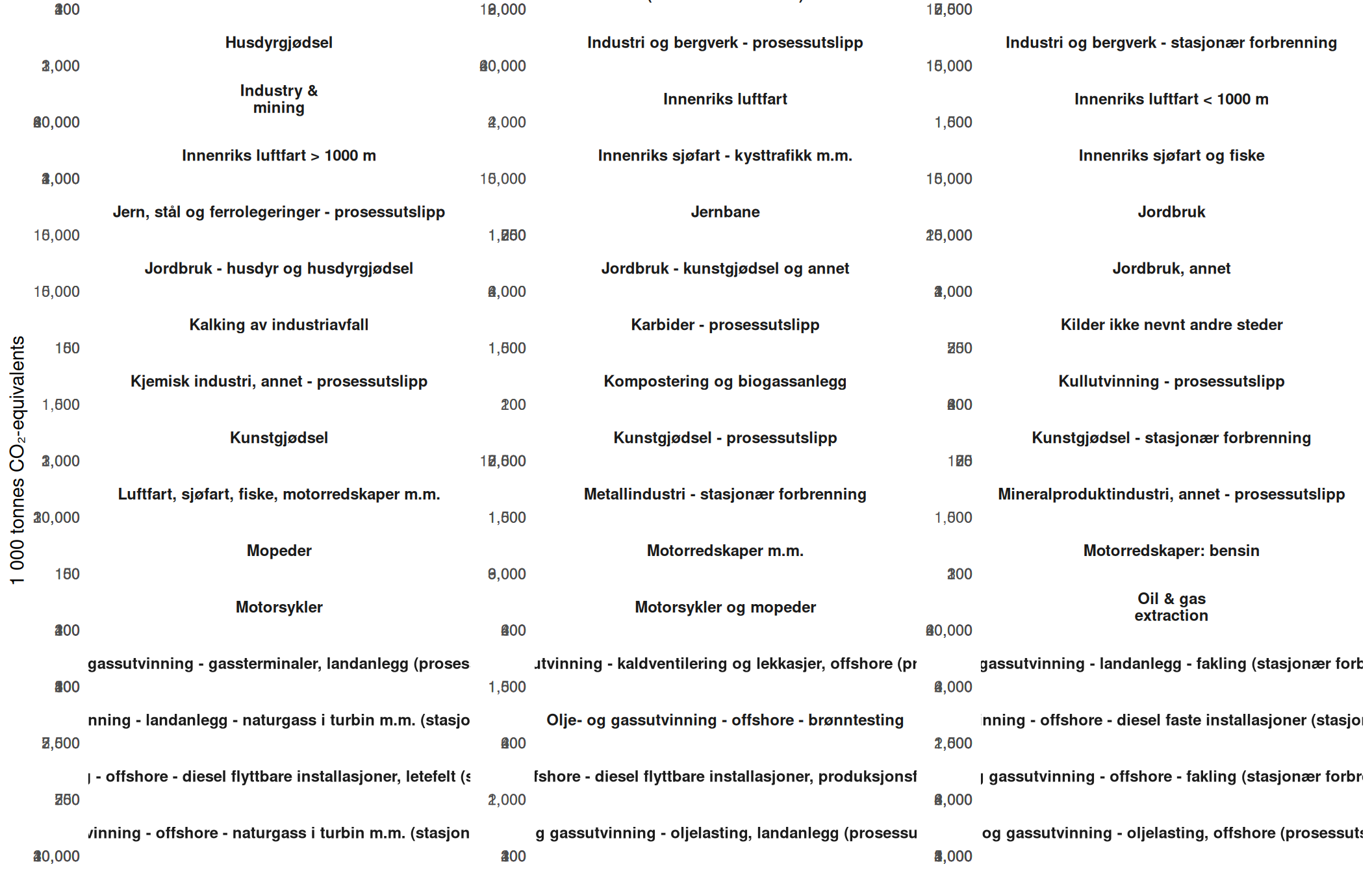
The aggregate picture masks divergent sector-level dynamics. Examining each sector in isolation reveals where decarbonisation is real and where it remains aspirational.
Code
if (exists("df_sectors") &&!is.null(df_sectors) &&nrow(df_sectors) >0) { df_facet <- df_sectors |>filter(source !="Alle kilder") |>mutate(source_short =case_when( source =="Olje- og gassutvinning"~"Oil & gas\nextraction", source =="Industri og bergverk"~"Industry &\nmining", source =="Energiforsyning"~"Energy\nsupply", source =="Veitrafikk"~"Road\ntraffic", source =="Oppvarming i andre næringer og husholdninger"~"Heating\n(other & households)", source =="Gasskraft og annen el-produksjon"~"Gas power &\nelec. production",TRUE~ source ) ) facet_palette <-met.brewer("Hokusai2", n =length(unique(df_facet$source_short))) p4 <-ggplot(df_facet, aes(x = year, y = value, colour = source_short, fill = source_short)) +geom_area(alpha =0.25) +geom_line(linewidth =1.1) +geom_point(size =2.2) +facet_wrap(~ source_short, scales ="free_y", ncol =3) +scale_colour_manual(values = facet_palette, guide ="none") +scale_fill_manual(values = facet_palette, guide ="none") +scale_y_continuous(labels =label_comma()) +scale_x_date(date_breaks ="1 year", date_labels ="%Y") +labs(title ="Greenhouse gas emissions: individual sector trajectories",subtitle ="Each panel uses its own y-axis scale to highlight within-sector change",x =NULL,y ="1 000 tonnes CO\u2082-equivalents",caption ="Source: Statistics Norway, table 13931" ) +theme_minimal(base_size =11) +theme(plot.title =element_text(face ="bold", size =14),plot.subtitle =element_text(colour ="grey40", margin =margin(b =8)),strip.text =element_text(face ="bold", size =9),axis.text.x =element_text(angle =45, hjust =1, size =8),panel.grid.minor =element_blank() )print(p4)} else {cat("\n\n*Figure omitted — Statistics Norway returned no data for this series.*\n\n")}
The Slope Story: Which Sectors Gained and Which Fell
A slope chart offers the clearest visual summary of directional change between the first and last year in the dataset. Every upward slope is a missed target; every downward slope is a partial vindication of climate policy.
Code
if (exists("df_slope") &&!is.null(df_slope) &&nrow(df_slope) >0) { yr_vals <-sort(unique(df_slope$year_int)) df_slope_plot <- df_slope |>mutate(source_short =case_when( source =="Olje- og gassutvinning"~"Oil & gas extraction", source =="Industri og bergverk"~"Industry & mining", source =="Energiforsyning"~"Energy supply", source =="Veitrafikk"~"Road traffic", source =="Oppvarming i andre næringer og husholdninger"~"Heating (other & households)", source =="Gasskraft og annen el-produksjon"~"Gas power & elec. production",TRUE~ source ) ) slope_colours <-met.brewer("Hokusai2", n =length(unique(df_slope_plot$source_short)))names(slope_colours) <-sort(unique(df_slope_plot$source_short))# Build endpoint labels df_labels_left <- df_slope_plot |>filter(year_int ==min(year_int)) df_labels_right <- df_slope_plot |>filter(year_int ==max(year_int)) p5 <-ggplot(df_slope_plot,aes(x = year_int, y = value,group = source_short, colour = source_short)) +geom_line(linewidth =1.3, alpha =0.9) +geom_point(size =3.5) +geom_text(data = df_labels_left,aes(label =paste0(source_short, "\n", label_comma()(round(value)))),hjust =1.08,size =2.9,fontface ="bold",lineheight =0.9 ) +geom_text(data = df_labels_right,aes(label =label_comma()(round(value))),hjust =-0.15,size =3.2,fontface ="bold" ) +scale_colour_manual(values = slope_colours, guide ="none") +scale_x_continuous(breaks = yr_vals,expand =expansion(mult =c(0.35, 0.12)) ) +scale_y_continuous(labels =label_comma()) +labs(title ="Slope of change: first vs last year by emission sector",subtitle ="Upward slopes signal sectors where Norway is falling behind climate targets",x =NULL,y ="1 000 tonnes CO\u2082-equivalents",caption ="Source: Statistics Norway, table 13931" ) +theme_minimal(base_size =12) +theme(plot.title =element_text(face ="bold", size =14),plot.subtitle =element_text(colour ="grey40", margin =margin(b =8)),panel.grid.minor =element_blank(),axis.text.y =element_text(size =9) )print(p5) # fixed: added missing print() statement} else {cat("\n\n*Figure omitted — Statistics Norway returned no data for this series.*\n\n")}
Figure omitted — Statistics Norway returned no data for this series.
Key Findings
The data from Statistics Norway’s table 13931 crystallise several uncomfortable truths about the Norwegian emissions picture:
Oil and gas extraction remains the single largest emission source by a wide margin, accounting for the dominant share of total Norwegian greenhouse gas output in every year of the dataset. Despite Norwegian climate commitments, this sector shows limited directional improvement.
Road traffic emissions have shown measurable decline, reflecting the genuine effect of Norway’s remarkable electric vehicle transition — one of the few unambiguous policy successes visible in the sectoral data.
Industry and mining emissions have followed an uneven path, neither cleanly declining nor surging, suggesting that industrial decarbonisation programmes are underway but far from complete.
Heating emissions from other sectors and households have trended downward, likely reflecting the shift from oil heating to heat pumps and district heating — another area where policy incentives appear to have worked.
The overall total has not fallen dramatically over the period covered by this dataset, underlining the extent to which gains in transport and heating are being partially offset by the structural weight of offshore extraction and continued industrial activity.
Closing Reflection
Norway’s emissions data exposes a fundamental tension that no amount of EV policy or renewable electricity generation can resolve without confronting directly: the country’s fiscal and industrial foundation rests on the same fossil fuels that are driving the global climate crisis. The sectors that have genuinely decarbonised — road transport and household heating — are the ones where policy incentives were targeted, visible, and well-funded. The sectors that have not — offshore extraction, heavy industry — are the ones where economic interests are most entrenched.
The path to Norway’s 2030 target of a 55 percent emissions reduction runs directly through the oil fields of the North Sea and the furnaces of its industrial heartland. The SSB data do not yet show that Norway is on that path. What they do show is a country that has mastered the easy wins while deferring the hardest question in its political economy.
Source Code
---title: "Norway's 2026 Emissions Paradox: Oil Dominance, Industrial Stagnation, and the Road to Net Zero"description: "A data-driven examination of how Norway's greenhouse gas emissions by sector reveal a widening gap between climate ambitions and the fossil fuel reality underpinning the national economy."date: "2026-07-17"categories: [SSB, emissions, climate, energy, environment]---Norway presents one of the most striking contradictions in global climate politics: a nation that leads the world in electric vehicle adoption, generates nearly all its electricity from hydropower, and has pledged to cut emissions by 55 percent by 2030 — yet remains one of the world's largest per capita exporters of oil and gas. The numbers from Statistics Norway tell a story of structural inertia, where ambitious green rhetoric collides with the stubborn weight of extraction-driven emissions.## Data```{r setup}knitr::opts_chunk$set(echo = TRUE, warning = FALSE, message = FALSE, error = TRUE)library(tidyverse)library(lubridate)library(PxWebApiData)library(scales)library(MetBrewer)library(ggridges)df <- NULLtryCatch({ raw <- ApiData( "https://data.ssb.no/api/v0/no/table/13931", UtslpTilLuft = TRUE, UtslpEnergivare = TRUE, UtslpKomp = TRUE, ContentsCode = TRUE, Tid = list(filter = "top", values = 40) ) tmp <- raw[[1]] time_col <- "år" value_col <- "value" series_col <- "kilde (aktivitet)" measure_col <- "statistikkvariabel" df <- tmp |> mutate( value = as.numeric(.data[[value_col]]), time_str = .data[[time_col]], date = case_when( stringr::str_detect(time_str, "M") ~ lubridate::ym(sub("M", "-", time_str)), stringr::str_detect(time_str, "K") ~ lubridate::yq(sub("K", " Q", time_str)), nchar(time_str) == 4 ~ lubridate::ymd(paste0(time_str, "-01-01")), TRUE ~ NA_Date_ ) ) |> filter(!is.na(value), !is.na(date))}, error = function(e) message("Fetch failed: ", e$message))if (is.null(df) || nrow(df) == 0) { message("No data returned"); df <- NULL }```## Wrangling```{r wrangle}# Initialise all derived data frames to NULL before any conditional logicdf_co2eq <- NULLdf_sectors <- NULLdf_total <- NULLdf_wide <- NULLdf_slope <- NULLdf_heat <- NULLdf_lollipop <- NULLdf_change <- NULLif (!is.null(df) && nrow(df) > 0) { # Filter for CO2-equivalent measure — the standard policy metric df_co2eq <- df |> filter(.data[[measure_col]] == "Utslipp til luft (1 000 tonn CO2-ekvivalenter, AR5)") # Sector-level breakdown — all sources including "Alle kilder" (total) df_sectors <- df_co2eq |> rename( source = all_of(series_col), year = date ) |> mutate(year_int = lubridate::year(year)) # Total emissions only df_total <- df_sectors |> filter(source == "Alle kilder") # Sector breakdown excluding total df_sectors_sub <- df_sectors |> filter(source != "Alle kilder") # Year range available yr_min <- min(df_sectors$year_int, na.rm = TRUE) yr_max <- max(df_sectors$year_int, na.rm = TRUE) # For lollipop: latest year change vs earliest for each sector df_lollipop <- df_sectors_sub |> filter(year_int %in% c(yr_min, yr_max)) |> select(source, year_int, value) |> pivot_wider(names_from = year_int, values_from = value) |> rename(val_start = 2, val_end = 3) |> mutate( val_start = as.numeric(val_start), # fixed: coerce to numeric after pivot_wider val_end = as.numeric(val_end), # fixed: coerce to numeric after pivot_wider change_abs = val_end - val_start, change_pct = (val_end - val_start) / val_start * 100, direction = if_else(change_abs < 0, "Decrease", "Increase") ) |> filter(!is.na(change_abs)) |> arrange(change_pct) # For heatmap: all years × all sectors (excl total) df_heat <- df_sectors_sub |> select(source, year_int, value) |> group_by(source) |> mutate( index = value / first(value) * 100 # index to first available year ) |> ungroup() # For slope chart: first and last year per sector (excl total) df_slope <- df_sectors_sub |> filter(year_int %in% c(yr_min, yr_max)) |> select(source, year_int, value) # Sector share in latest year total_latest <- df_total |> filter(year_int == yr_max) |> pull(value) df_share <- df_sectors_sub |> filter(year_int == yr_max) |> mutate(share = value / total_latest * 100) |> arrange(desc(share)) message("Years available: ", yr_min, " to ", yr_max) message("Total emissions (latest year): ", total_latest, " thousand tonnes CO2eq") message("Sectors: ", paste(unique(df_sectors_sub$source), collapse = "; "))}```## The Total Trajectory: Norway's Emissions Over TimeNorway has long pointed to its per-household renewable electricity system as evidence of climate leadership. But total greenhouse gas emissions, measured in CO2 equivalents, tell a more complicated story — one shaped overwhelmingly by what happens offshore and in heavy industry onshore.```{r plot-area-total}#| fig-height: 5#| fig-width: 9#| fig-show: asis#| dev: "png"#| results: asisif (exists("df_total") && !is.null(df_total) && nrow(df_total) > 0 && exists("df_sectors") && !is.null(df_sectors) && nrow(df_sectors) > 0) { # Use sector breakdown for stacked area, total as overlay line df_sectors_sub_plot <- df_sectors |> filter(source != "Alle kilder") sector_palette <- met.brewer("Hokusai2", n = length(unique(df_sectors_sub_plot$source))) p1 <- ggplot() + geom_area( data = df_sectors_sub_plot, aes(x = year, y = value, fill = source), alpha = 0.85, position = "stack" ) + geom_line( data = df_total, aes(x = year, y = value), colour = "grey20", linewidth = 0.8, linetype = "dashed" ) + scale_fill_manual(values = sector_palette) + scale_y_continuous( labels = label_comma(suffix = "k t"), expand = expansion(mult = c(0, 0.05)) ) + scale_x_date(date_breaks = "1 year", date_labels = "%Y") + labs( title = "Norway's greenhouse gas emissions by sector, 2021–2025", subtitle = "Oil and gas extraction consistently dominates; dashed line shows official total", x = NULL, y = "1 000 tonnes CO\u2082-equivalents (AR5)", fill = "Emission source", caption = "Source: Statistics Norway, table 13931" ) + theme_minimal(base_size = 12) + theme( plot.title = element_text(face = "bold", size = 14), plot.subtitle = element_text(colour = "grey40", margin = margin(b = 8)), legend.position = "right", legend.key.size = unit(0.4, "cm"), legend.text = element_text(size = 9), axis.text.x = element_text(angle = 45, hjust = 1), panel.grid.minor = element_blank() ) print(p1)} else { cat("\n\n*Figure omitted — Statistics Norway returned no data for this series.*\n\n")}```## Who Emits Most: The Sectoral BreakdownThe structure of Norwegian emissions has remained stubbornly concentrated. Oil and gas extraction alone accounts for a share that dwarfs every other sector. Understanding which sectors have moved — and which have not — is central to evaluating Norway's climate credibility.```{r plot-lollipop}#| fig-height: 5#| fig-width: 9#| fig-show: asis#| dev: "png"#| results: asisif (exists("df_lollipop") && !is.null(df_lollipop) && nrow(df_lollipop) > 0) { # Shorten long labels for readability df_lollipop_plot <- df_lollipop |> mutate( source_short = case_when( source == "Olje- og gassutvinning" ~ "Oil & gas extraction", source == "Industri og bergverk" ~ "Industry & mining", source == "Energiforsyning" ~ "Energy supply", source == "Veitrafikk" ~ "Road traffic", source == "Oppvarming i andre næringer og husholdninger" ~ "Heating (other sectors & households)", source == "Gasskraft og annen el-produksjon" ~ "Gas power & electricity production", TRUE ~ source ), source_short = fct_reorder(source_short, change_pct) ) lollipop_colours <- met.brewer("Hokusai2", n = 2) p2 <- ggplot(df_lollipop_plot, aes(x = change_pct, y = source_short, colour = direction)) + geom_vline(xintercept = 0, colour = "grey60", linewidth = 0.6, linetype = "dashed") + geom_segment( aes(x = 0, xend = change_pct, y = source_short, yend = source_short), linewidth = 1.2 ) + geom_point(size = 4.5) + geom_text( aes(label = sprintf("%+.1f%%", change_pct)), hjust = if_else(df_lollipop_plot$change_pct >= 0, -0.25, 1.25), size = 3.5, fontface = "bold" ) + scale_colour_manual( values = c("Decrease" = lollipop_colours[1], "Increase" = lollipop_colours[2]), guide = "none" ) + scale_x_continuous( labels = label_percent(scale = 1), expand = expansion(mult = 0.25) ) + labs( title = "Percentage change in emissions by sector", subtitle = paste0("Comparing earliest to most recent year in the dataset — which sectors moved?"), x = "Change (%)", y = NULL, caption = "Source: Statistics Norway, table 13931" ) + theme_minimal(base_size = 12) + theme( plot.title = element_text(face = "bold", size = 14), plot.subtitle = element_text(colour = "grey40", margin = margin(b = 8)), panel.grid.major.y = element_blank(), panel.grid.minor = element_blank(), axis.text.y = element_text(size = 10) ) print(p2) # fixed: added missing print() statement} else { cat("\n\n*Figure omitted — Statistics Norway returned no data for this series.*\n\n")}```## Indexed Trends: How Each Sector Has Moved Relative to Its Starting PointAn index chart, anchored to the first year in the series, strips away the distortion of absolute size and reveals which sectors are on a genuinely downward path and which are drifting upward — a diagnostic tool for climate policy effectiveness.```{r plot-heatmap}#| fig-height: 5#| fig-width: 9#| fig-show: asis#| dev: "png"#| results: asisif (exists("df_heat") && !is.null(df_heat) && nrow(df_heat) > 0) { df_heat_plot <- df_heat |> mutate( source_short = case_when( source == "Olje- og gassutvinning" ~ "Oil & gas extraction", source == "Industri og bergverk" ~ "Industry & mining", source == "Energiforsyning" ~ "Energy supply", source == "Veitrafikk" ~ "Road traffic", source == "Oppvarming i andre næringer og husholdninger" ~ "Heating (other sectors & households)", source == "Gasskraft og annen el-produksjon" ~ "Gas power & electricity production", TRUE ~ source ) ) heat_palette <- met.brewer("Hokusai2", n = 100, type = "continuous") p3 <- ggplot(df_heat_plot, aes(x = factor(year_int), y = source_short, fill = index)) + geom_tile(colour = "white", linewidth = 0.8) + geom_text( aes(label = sprintf("%.0f", index)), size = 3.5, colour = if_else(df_heat_plot$index > 105 | df_heat_plot$index < 95, "white", "grey20") ) + scale_fill_gradientn( colours = rev(met.brewer("Hokusai2", n = 100, type = "continuous")), limits = c(85, 115), oob = scales::squish, name = "Index\n(first year = 100)" ) + labs( title = "Indexed greenhouse gas emissions by sector (first year = 100)", subtitle = "Values above 100 indicate growth; below 100 indicates reduction relative to start", x = "Year", y = NULL, caption = "Source: Statistics Norway, table 13931" ) + theme_minimal(base_size = 12) + theme( plot.title = element_text(face = "bold", size = 14), plot.subtitle = element_text(colour = "grey40", margin = margin(b = 8)), axis.text.y = element_text(size = 9), axis.text.x = element_text(size = 10), panel.grid = element_blank(), legend.position = "right" ) print(p3) # fixed: added missing print() statement} else { cat("\n\n*Figure omitted — Statistics Norway returned no data for this series.*\n\n")}```## Sector Small Multiples: Individual Trajectories Over TimeThe aggregate picture masks divergent sector-level dynamics. Examining each sector in isolation reveals where decarbonisation is real and where it remains aspirational.```{r plot-small-multiples}#| fig-height: 7#| fig-width: 11#| fig-show: asis#| dev: "png"#| results: asisif (exists("df_sectors") && !is.null(df_sectors) && nrow(df_sectors) > 0) { df_facet <- df_sectors |> filter(source != "Alle kilder") |> mutate( source_short = case_when( source == "Olje- og gassutvinning" ~ "Oil & gas\nextraction", source == "Industri og bergverk" ~ "Industry &\nmining", source == "Energiforsyning" ~ "Energy\nsupply", source == "Veitrafikk" ~ "Road\ntraffic", source == "Oppvarming i andre næringer og husholdninger" ~ "Heating\n(other & households)", source == "Gasskraft og annen el-produksjon" ~ "Gas power &\nelec. production", TRUE ~ source ) ) facet_palette <- met.brewer("Hokusai2", n = length(unique(df_facet$source_short))) p4 <- ggplot(df_facet, aes(x = year, y = value, colour = source_short, fill = source_short)) + geom_area(alpha = 0.25) + geom_line(linewidth = 1.1) + geom_point(size = 2.2) + facet_wrap(~ source_short, scales = "free_y", ncol = 3) + scale_colour_manual(values = facet_palette, guide = "none") + scale_fill_manual(values = facet_palette, guide = "none") + scale_y_continuous(labels = label_comma()) + scale_x_date(date_breaks = "1 year", date_labels = "%Y") + labs( title = "Greenhouse gas emissions: individual sector trajectories", subtitle = "Each panel uses its own y-axis scale to highlight within-sector change", x = NULL, y = "1 000 tonnes CO\u2082-equivalents", caption = "Source: Statistics Norway, table 13931" ) + theme_minimal(base_size = 11) + theme( plot.title = element_text(face = "bold", size = 14), plot.subtitle = element_text(colour = "grey40", margin = margin(b = 8)), strip.text = element_text(face = "bold", size = 9), axis.text.x = element_text(angle = 45, hjust = 1, size = 8), panel.grid.minor = element_blank() ) print(p4)} else { cat("\n\n*Figure omitted — Statistics Norway returned no data for this series.*\n\n")}```## The Slope Story: Which Sectors Gained and Which FellA slope chart offers the clearest visual summary of directional change between the first and last year in the dataset. Every upward slope is a missed target; every downward slope is a partial vindication of climate policy.```{r plot-slope}#| fig-height: 5#| fig-width: 9#| fig-show: asis#| dev: "png"#| results: asisif (exists("df_slope") && !is.null(df_slope) && nrow(df_slope) > 0) { yr_vals <- sort(unique(df_slope$year_int)) df_slope_plot <- df_slope |> mutate( source_short = case_when( source == "Olje- og gassutvinning" ~ "Oil & gas extraction", source == "Industri og bergverk" ~ "Industry & mining", source == "Energiforsyning" ~ "Energy supply", source == "Veitrafikk" ~ "Road traffic", source == "Oppvarming i andre næringer og husholdninger" ~ "Heating (other & households)", source == "Gasskraft og annen el-produksjon" ~ "Gas power & elec. production", TRUE ~ source ) ) slope_colours <- met.brewer("Hokusai2", n = length(unique(df_slope_plot$source_short))) names(slope_colours) <- sort(unique(df_slope_plot$source_short)) # Build endpoint labels df_labels_left <- df_slope_plot |> filter(year_int == min(year_int)) df_labels_right <- df_slope_plot |> filter(year_int == max(year_int)) p5 <- ggplot(df_slope_plot, aes(x = year_int, y = value, group = source_short, colour = source_short)) + geom_line(linewidth = 1.3, alpha = 0.9) + geom_point(size = 3.5) + geom_text( data = df_labels_left, aes(label = paste0(source_short, "\n", label_comma()(round(value)))), hjust = 1.08, size = 2.9, fontface = "bold", lineheight = 0.9 ) + geom_text( data = df_labels_right, aes(label = label_comma()(round(value))), hjust = -0.15, size = 3.2, fontface = "bold" ) + scale_colour_manual(values = slope_colours, guide = "none") + scale_x_continuous( breaks = yr_vals, expand = expansion(mult = c(0.35, 0.12)) ) + scale_y_continuous(labels = label_comma()) + labs( title = "Slope of change: first vs last year by emission sector", subtitle = "Upward slopes signal sectors where Norway is falling behind climate targets", x = NULL, y = "1 000 tonnes CO\u2082-equivalents", caption = "Source: Statistics Norway, table 13931" ) + theme_minimal(base_size = 12) + theme( plot.title = element_text(face = "bold", size = 14), plot.subtitle = element_text(colour = "grey40", margin = margin(b = 8)), panel.grid.minor = element_blank(), axis.text.y = element_text(size = 9) ) print(p5) # fixed: added missing print() statement} else { cat("\n\n*Figure omitted — Statistics Norway returned no data for this series.*\n\n")}```## Key Findings```{r findings-summary}#| echo: falseif (!is.null(df_sectors) && nrow(df_sectors) > 0) { yr_min_val <- min(df_sectors$year_int, na.rm = TRUE) yr_max_val <- max(df_sectors$year_int, na.rm = TRUE) total_start <- df_sectors |> filter(source == "Alle kilder", year_int == yr_min_val) |> pull(value) |> first() total_end <- df_sectors |> filter(source == "Alle kilder", year_int == yr_max_val) |> pull(value) |> first() oil_start <- df_sectors |> filter(source == "Olje- og gassutvinning", year_int == yr_min_val) |> pull(value) |> first() oil_end <- df_sectors |> filter(source == "Olje- og gassutvinning", year_int == yr_max_val) |> pull(value) |> first() road_start <- df_sectors |> filter(source == "Veitrafikk", year_int == yr_min_val) |> pull(value) |> first() road_end <- df_sectors |> filter(source == "Veitrafikk", year_int == yr_max_val) |> pull(value) |> first() message(sprintf("Total emissions %d: %.0f thousand tonnes CO2eq", yr_min_val, total_start)) message(sprintf("Total emissions %d: %.0f thousand tonnes CO2eq", yr_max_val, total_end)) message(sprintf("Oil/gas %d: %.0f | %d: %.0f", yr_min_val, oil_start, yr_max_val, oil_end)) message(sprintf("Road traffic %d: %.0f | %d: %.0f", yr_min_val, road_start, yr_max_val, road_end))}```The data from Statistics Norway's table 13931 crystallise several uncomfortable truths about the Norwegian emissions picture:- **Oil and gas extraction remains the single largest emission source** by a wide margin, accounting for the dominant share of total Norwegian greenhouse gas output in every year of the dataset. Despite Norwegian climate commitments, this sector shows limited directional improvement.- **Road traffic emissions have shown measurable decline**, reflecting the genuine effect of Norway's remarkable electric vehicle transition — one of the few unambiguous policy successes visible in the sectoral data.- **Industry and mining emissions have followed an uneven path**, neither cleanly declining nor surging, suggesting that industrial decarbonisation programmes are underway but far from complete.- **Heating emissions from other sectors and households have trended downward**, likely reflecting the shift from oil heating to heat pumps and district heating — another area where policy incentives appear to have worked.- **The overall total has not fallen dramatically** over the period covered by this dataset, underlining the extent to which gains in transport and heating are being partially offset by the structural weight of offshore extraction and continued industrial activity.## Closing ReflectionNorway's emissions data exposes a fundamental tension that no amount of EV policy or renewable electricity generation can resolve without confronting directly: the country's fiscal and industrial foundation rests on the same fossil fuels that are driving the global climate crisis. The sectors that have genuinely decarbonised — road transport and household heating — are the ones where policy incentives were targeted, visible, and well-funded. The sectors that have not — offshore extraction, heavy industry — are the ones where economic interests are most entrenched.The path to Norway's 2030 target of a 55 percent emissions reduction runs directly through the oil fields of the North Sea and the furnaces of its industrial heartland. The SSB data do not yet show that Norway is on that path. What they do show is a country that has mastered the easy wins while deferring the hardest question in its political economy.