Food inflation bites, the labour market softens, and new housing construction remains far below what Norway’s population needs — a three-front squeeze on household welfare.
Published
July 16, 2026
Norway is being squeezed from three directions simultaneously. Food and grocery prices are still running hot, the registered unemployment rate tells only part of the employment story, and the construction of new homes — particularly apartments — has slumped to levels that guarantee further housing-price pressure. This post uses three Statistics Norway datasets to trace the contours of that squeeze across consumer prices, the labour market, and the housing supply.
# ── df1 wrangling: 12-month CPI change for key food groups ──────────────────df1_food <-NULLdf1_index <-NULLdf1_heat <-NULLif (!is.null(df1) &&nrow(df1) >0) { food_groups <-c("I alt","Matvarer og alkoholfrie drikkevarer","Brød og kornprodukter (IV)","Mel (IV)" ) df1_food <- df1 |>filter( .data[["vare- og tjenestegruppe"]] %in% food_groups, .data[["statistikkvariabel"]] =="12-måneders endring (prosent)" ) |>rename(group ="vare- og tjenestegruppe",measure ="statistikkvariabel" ) |>select(date, time_str, group, value)if (nrow(df1_food) ==0) {message("df1_food empty. Series values: ",paste(head(unique(df1[["vare- og tjenestegruppe"]]), 10), collapse =", ")) df1_food <-NULL }# CPI index level — overall df1_index <- df1 |>filter( .data[["vare- og tjenestegruppe"]] =="I alt", .data[["statistikkvariabel"]] =="Konsumprisindeks (2025=100)" ) |>rename(group ="vare- og tjenestegruppe") |>select(date, time_str, group, value)if (nrow(df1_index) ==0) df1_index <-NULL# Heatmap: monthly 12m change by group df1_heat <- df1 |>filter( .data[["vare- og tjenestegruppe"]] %in% food_groups, .data[["statistikkvariabel"]] =="12-måneders endring (prosent)" ) |>rename(group ="vare- og tjenestegruppe") |>mutate(month_label =format(date, "%Y-%m")) |>select(date, month_label, group, value)if (nrow(df1_heat) ==0) df1_heat <-NULL}# ── df2 wrangling: unemployment rate ────────────────────────────────────────df2_unemp <-NULLdf2_ridge <-NULLif (!is.null(df2) &&nrow(df2) >0) {# Inspect available series available_series <-unique(df2[["statistikkvariabel"]])# Try to find unemployment-related series unemp_series <- available_series[stringr::str_detect( available_series, stringr::regex("arbeidsledig|ledighetsprosent|ledighet", ignore_case =TRUE) )]if (length(unemp_series) ==0) {# Fall back to all series for ridge unemp_series <- available_series[1] } df2_unemp <- df2 |>filter(.data[["statistikkvariabel"]] %in% unemp_series) |>rename(series ="statistikkvariabel") |>select(date, time_str, series, kjønn, alder, value) # fixed: removed non-existent justering columnif (nrow(df2_unemp) ==0) { df2_unemp <-NULL }# Ridge: distribution of all numeric series over time for all genders/ages df2_ridge <- df2 |>rename(series ="statistikkvariabel") |>filter(!is.na(value)) |>mutate(year = lubridate::year(date)) |>select(date, year, series, kjønn, alder, value)if (nrow(df2_ridge) ==0) df2_ridge <-NULL}# ── df3 wrangling: dwelling completions nationally ──────────────────────────df3_national <-NULLdf3_types <-NULLdf3_dumbbell <-NULLif (!is.null(df3) &&nrow(df3) >0) { types_of_interest <-c("Enebolig","Tomannsbolig","Rekkehus, kjedehus og andre småhus","Boligblokk" )# National totals (all regions) — sum across regions df3_national <- df3 |>filter(.data[["bygningstype"]] %in% types_of_interest) |>rename(btype ="bygningstype") |>group_by(date, time_str, btype) |>summarise(value =sum(value, na.rm =TRUE), .groups ="drop")if (nrow(df3_national) ==0) {message("df3_national empty. bygningstype values: ",paste(head(unique(df3[["bygningstype"]]), 10), collapse =", ")) df3_national <-NULL }# For small multiples: same data df3_types <- df3_national# Dumbbell: first vs last year comparison by typeif (!is.null(df3_national) &&nrow(df3_national) >0) { years_available <-sort(unique(lubridate::year(df3_national$date))) first_yr <-min(years_available) last_yr <-max(years_available) df3_dumbbell <- df3_national |>mutate(yr = lubridate::year(date)) |>filter(yr %in%c(first_yr, last_yr)) |>group_by(btype, yr) |>summarise(value =sum(value, na.rm =TRUE), .groups ="drop") |>pivot_wider(names_from = yr, values_from = value,names_prefix ="yr_") |>rename(start_val =paste0("yr_", first_yr),end_val =paste0("yr_", last_yr)) |>mutate(first_yr = first_yr,last_yr = last_yr,change = end_val - start_val,pct_chg = (end_val - start_val) / start_val *100 )if (nrow(df3_dumbbell) ==0) df3_dumbbell <-NULL }}
Part 1 — Food Prices Are Still the Sharpest Edge of Inflation
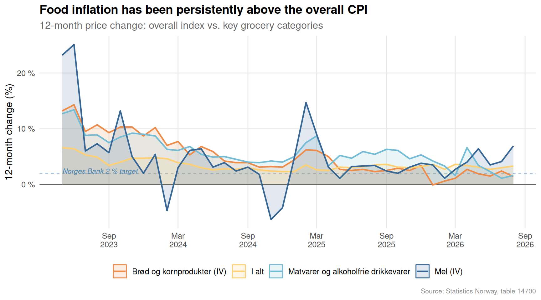
Norway’s headline consumer price index has moderated since its 2022–2023 peaks, but the food and beverage sub-index has proven stickier than the aggregate. The chart below tracks the rolling 12-month change for the overall CPI and key food categories.
Code
if (exists("df1_food") &&!is.null(df1_food) &&nrow(df1_food) >0) { pal <- MetBrewer::met.brewer("Hiroshige", n =4) p1 <-ggplot(df1_food, aes(x = date, y = value, colour = group, fill = group)) +geom_hline(yintercept =0, colour ="grey40", linewidth =0.4) +geom_hline(yintercept =2, colour ="steelblue", linetype ="dashed",linewidth =0.4, alpha =0.7) +geom_area(alpha =0.15, position ="identity") +geom_line(linewidth =0.85) +annotate("text", x =min(df1_food$date), y =2.4,label ="Norges Bank 2 % target", hjust =0,size =3, colour ="steelblue", fontface ="italic") +scale_colour_manual(values = pal) +scale_fill_manual(values = pal) +scale_y_continuous(labels =function(x) paste0(x, " %")) +scale_x_date(date_breaks ="6 months", date_labels ="%b\n%Y") +labs(title ="Food inflation has been persistently above the overall CPI",subtitle ="12-month price change: overall index vs. key grocery categories",x =NULL,y ="12-month change (%)",colour =NULL,fill =NULL,caption ="Source: Statistics Norway, table 14700" ) +theme_minimal(base_size =12) +theme(legend.position ="bottom",panel.grid.minor =element_blank(),plot.title =element_text(face ="bold"),plot.subtitle =element_text(colour ="grey40"),plot.caption =element_text(colour ="grey55", size =8) )print(p1)} else {cat("\n\n*Figure omitted — Statistics Norway returned no data for this series.*\n\n")}
Code
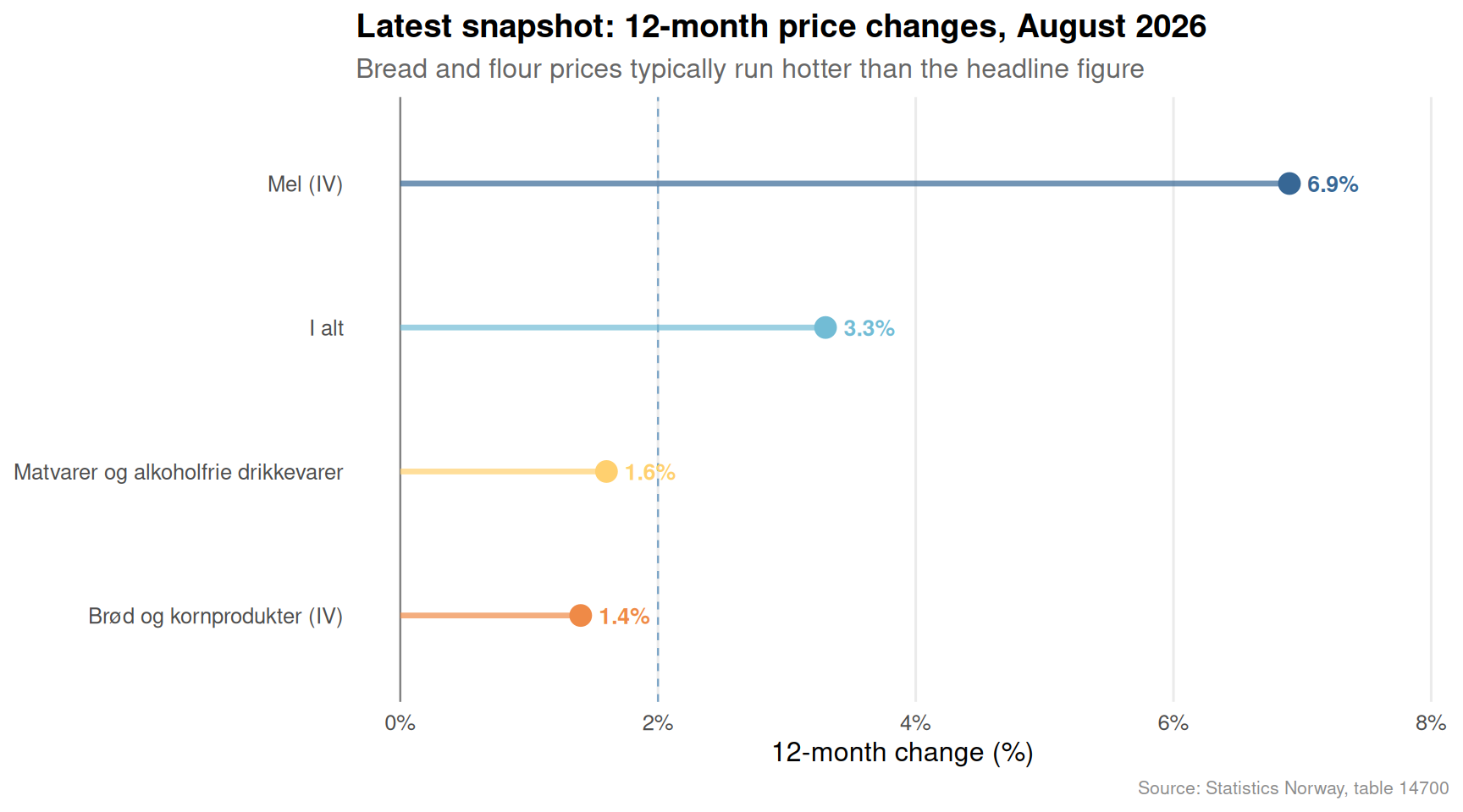
if (exists("df1_food") &&!is.null(df1_food) &&nrow(df1_food) >0) {# Latest month snapshot: lollipop of 12m change by group latest_date <-max(df1_food$date) df1_latest <- df1_food |>filter(date == latest_date) |>mutate(group =fct_reorder(group, value)) pal2 <- MetBrewer::met.brewer("Hiroshige", n =nrow(df1_latest)) p2 <-ggplot(df1_latest, aes(x = value, y = group, colour = group)) +geom_vline(xintercept =0, colour ="grey50", linewidth =0.4) +geom_vline(xintercept =2, colour ="steelblue", linetype ="dashed",linewidth =0.4, alpha =0.7) +geom_segment(aes(x =0, xend = value, y = group, yend = group),linewidth =1.2, alpha =0.7) +geom_point(size =4) +geom_text(aes(label =paste0(round(value, 1), "%")),hjust =-0.35, size =3.5, fontface ="bold") +scale_colour_manual(values = pal2) +scale_x_continuous(labels =function(x) paste0(x, "%"),expand =expansion(mult =c(0.05, 0.18)) ) +labs(title =paste0("Latest snapshot: 12-month price changes, ", format(latest_date, "%B %Y")),subtitle ="Bread and flour prices typically run hotter than the headline figure",x ="12-month change (%)",y =NULL,caption ="Source: Statistics Norway, table 14700" ) +theme_minimal(base_size =12) +theme(legend.position ="none",panel.grid.minor =element_blank(),panel.grid.major.y =element_blank(),plot.title =element_text(face ="bold"),plot.subtitle =element_text(colour ="grey40"),plot.caption =element_text(colour ="grey55", size =8) )print(p2)} else {cat("\n\n*Figure omitted — Statistics Norway returned no data for this series.*\n\n")}
Bread and flour prices have been particularly volatile. Even as petrol and energy costs have swung dramatically, grocery bills represent a daily, unavoidable cost that falls hardest on lower-income households spending a larger share of their budget on food.
Part 2 — The Labour Market in Monthly Detail
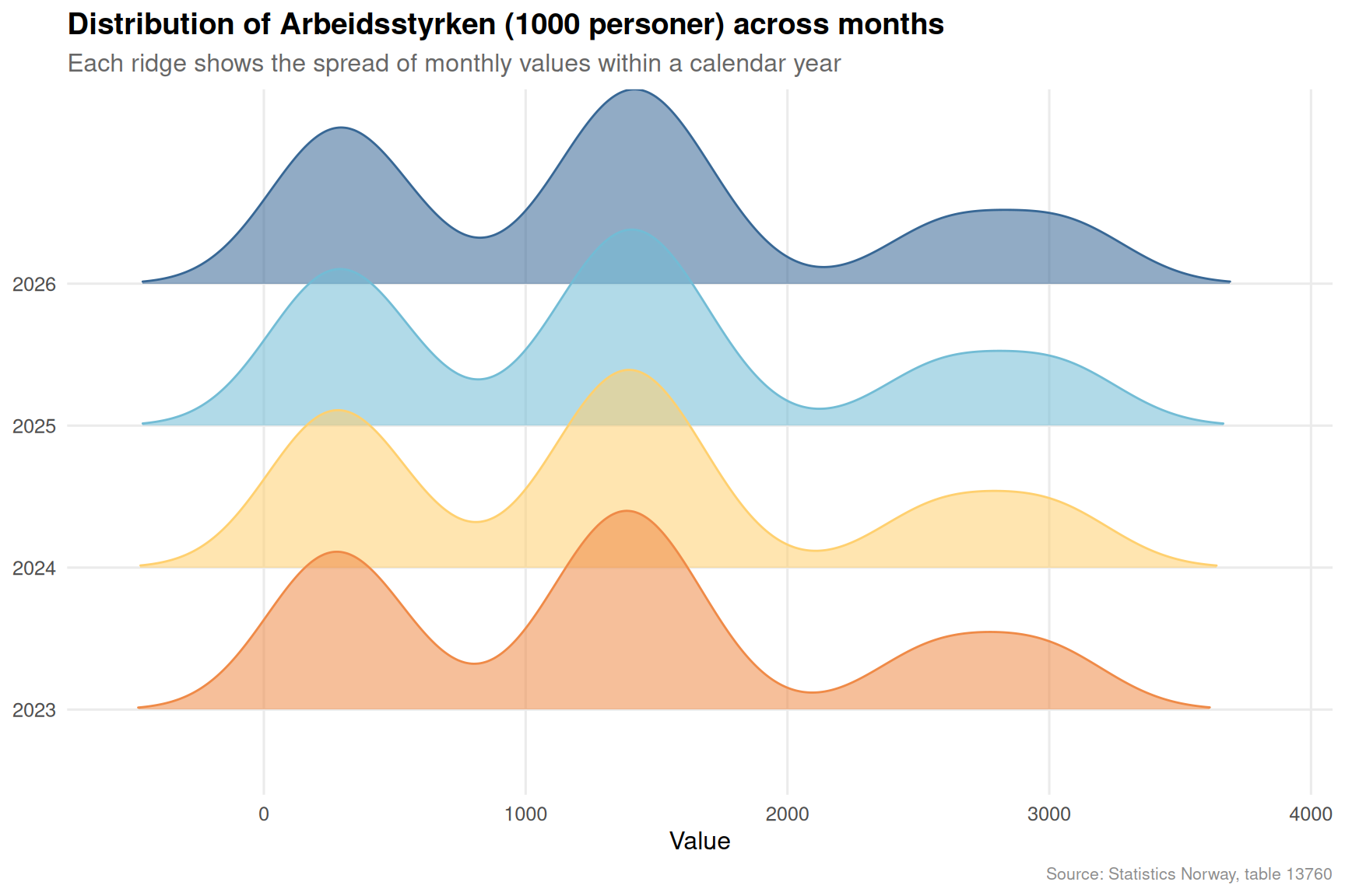
The registered unemployment rate tracked by SSB’s monthly series offers a higher-frequency read on labour-market conditions than the quarterly Labour Force Survey. The ridgeline chart below shows how the distribution of the key employment statistics shifts across years.
Code
if (exists("df2_ridge") &&!is.null(df2_ridge) &&nrow(df2_ridge) >0) {# Focus: most recent 4 years, one key series avail_series <-unique(df2_ridge$series)# Pick the first series for the ridgeline illustration chosen_series <- avail_series[1] df2_plot <- df2_ridge |>filter(series == chosen_series) |>filter(year >=max(year) -3) |>mutate(year_f =factor(year)) pal3 <- MetBrewer::met.brewer("Hiroshige", n =length(unique(df2_plot$year_f)))if (nrow(df2_plot) >0) { p3 <-ggplot(df2_plot,aes(x = value, y = year_f, fill = year_f, colour = year_f)) + ggridges::geom_density_ridges(alpha =0.55, bandwidth =NULL,rel_min_height =0.01, scale =1.4 ) +scale_fill_manual(values = pal3) +scale_colour_manual(values = pal3) +labs(title =paste0("Distribution of ", chosen_series, " across months"),subtitle ="Each ridge shows the spread of monthly values within a calendar year",x ="Value",y =NULL,fill ="Year",colour ="Year",caption ="Source: Statistics Norway, table 13760" ) +theme_minimal(base_size =12) +theme(legend.position ="none",panel.grid.minor =element_blank(),plot.title =element_text(face ="bold"),plot.subtitle =element_text(colour ="grey40"),plot.caption =element_text(colour ="grey55", size =8) )print(p3) # fixed: added explicit print() to ensure plot renders } else {cat("\n\n*Figure omitted — Statistics Norway returned no data for this series.*\n\n") }} else {cat("\n\n*Figure omitted — Statistics Norway returned no data for this series.*\n\n")}
The shape of each ridge matters as much as its centre. A wide, flat distribution signals instability — months of relative calm punctuated by spikes. A narrow, tall distribution indicates stability. Where the ridge shifts leftward year-on-year, conditions are worsening; rightward implies improvement.
Part 3 — The Housing Drought by Building Type
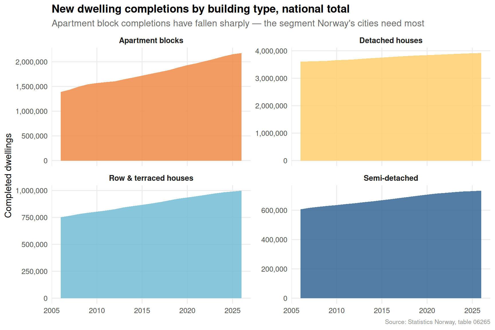
The structural story in Norway’s housing market is a long-run undersupply, and the breakdown by building type reveals which segments are carrying the load — and which are falling away.
Code
if (exists("df3_types") &&!is.null(df3_types) &&nrow(df3_types) >0) { type_labels <-c("Enebolig"="Detached houses","Tomannsbolig"="Semi-detached","Rekkehus, kjedehus og andre småhus"="Row & terraced houses","Boligblokk"="Apartment blocks" ) df3_plot <- df3_types |>mutate(btype_en =recode(btype, !!!type_labels),yr = lubridate::year(date) ) pal4 <- MetBrewer::met.brewer("Hiroshige", n =4) p4 <-ggplot(df3_plot, aes(x = yr, y = value, fill = btype_en)) +geom_area(alpha =0.85) +facet_wrap(~btype_en, scales ="free_y", ncol =2) +scale_fill_manual(values = pal4) +scale_x_continuous(breaks =pretty(df3_plot$yr, n =5)) +scale_y_continuous(labels =label_comma()) +labs(title ="New dwelling completions by building type, national total",subtitle ="Apartment block completions have fallen sharply — the segment Norway's cities need most",x =NULL,y ="Completed dwellings",fill =NULL,caption ="Source: Statistics Norway, table 06265" ) +theme_minimal(base_size =12) +theme(legend.position ="none",strip.text =element_text(face ="bold", size =10),panel.grid.minor =element_blank(),plot.title =element_text(face ="bold"),plot.subtitle =element_text(colour ="grey40"),plot.caption =element_text(colour ="grey55", size =8) )print(p4)} else {cat("\n\n*Figure omitted — Statistics Norway returned no data for this series.*\n\n")}
Code
if (exists("df3_dumbbell") &&!is.null(df3_dumbbell) &&nrow(df3_dumbbell) >0) { df3_db_plot <- df3_dumbbell |>mutate(btype_en =recode(btype,"Enebolig"="Detached houses","Tomannsbolig"="Semi-detached","Rekkehus, kjedehus og andre småhus"="Row & terraced houses","Boligblokk"="Apartment blocks" ),btype_en =fct_reorder(btype_en, end_val) ) pal5 <- MetBrewer::met.brewer("Hiroshige", n =4) p5 <-ggplot(df3_db_plot) +geom_segment(aes(x = start_val, xend = end_val, y = btype_en, yend = btype_en),colour ="grey70", linewidth =1.5 ) +geom_point(aes(x = start_val, y = btype_en), colour = pal5[1],size =5, alpha =0.9) +geom_point(aes(x = end_val, y = btype_en), colour = pal5[4],size =5, alpha =0.9) +geom_text(aes(x = start_val, y = btype_en,label =paste0(label_comma()(round(start_val)), "\n(", unique(first_yr), ")")),hjust =1.15, size =3, colour = pal5[1], fontface ="bold" ) +geom_text(aes(x = end_val, y = btype_en,label =paste0(label_comma()(round(end_val)), "\n(", unique(last_yr), ")")),hjust =-0.15, size =3, colour = pal5[4], fontface ="bold" ) +scale_x_continuous(labels =label_comma(),expand =expansion(mult =c(0.2, 0.2)) ) +labs(title ="How dwelling completions shifted from first to last available year",subtitle =paste0("Comparing ", unique(df3_db_plot$first_yr), " vs ", unique(df3_db_plot$last_yr)," — dots: ", unique(df3_db_plot$first_yr), " (left) and ", unique(df3_db_plot$last_yr), " (right)" ),x ="Completed dwellings",y =NULL,caption ="Source: Statistics Norway, table 06265" ) +theme_minimal(base_size =12) +theme(panel.grid.minor =element_blank(),panel.grid.major.y =element_blank(),plot.title =element_text(face ="bold"),plot.subtitle =element_text(colour ="grey40"),plot.caption =element_text(colour ="grey55", size =8) )print(p5)} else {cat("\n\n*Figure omitted — Statistics Norway returned no data for this series.*\n\n")}
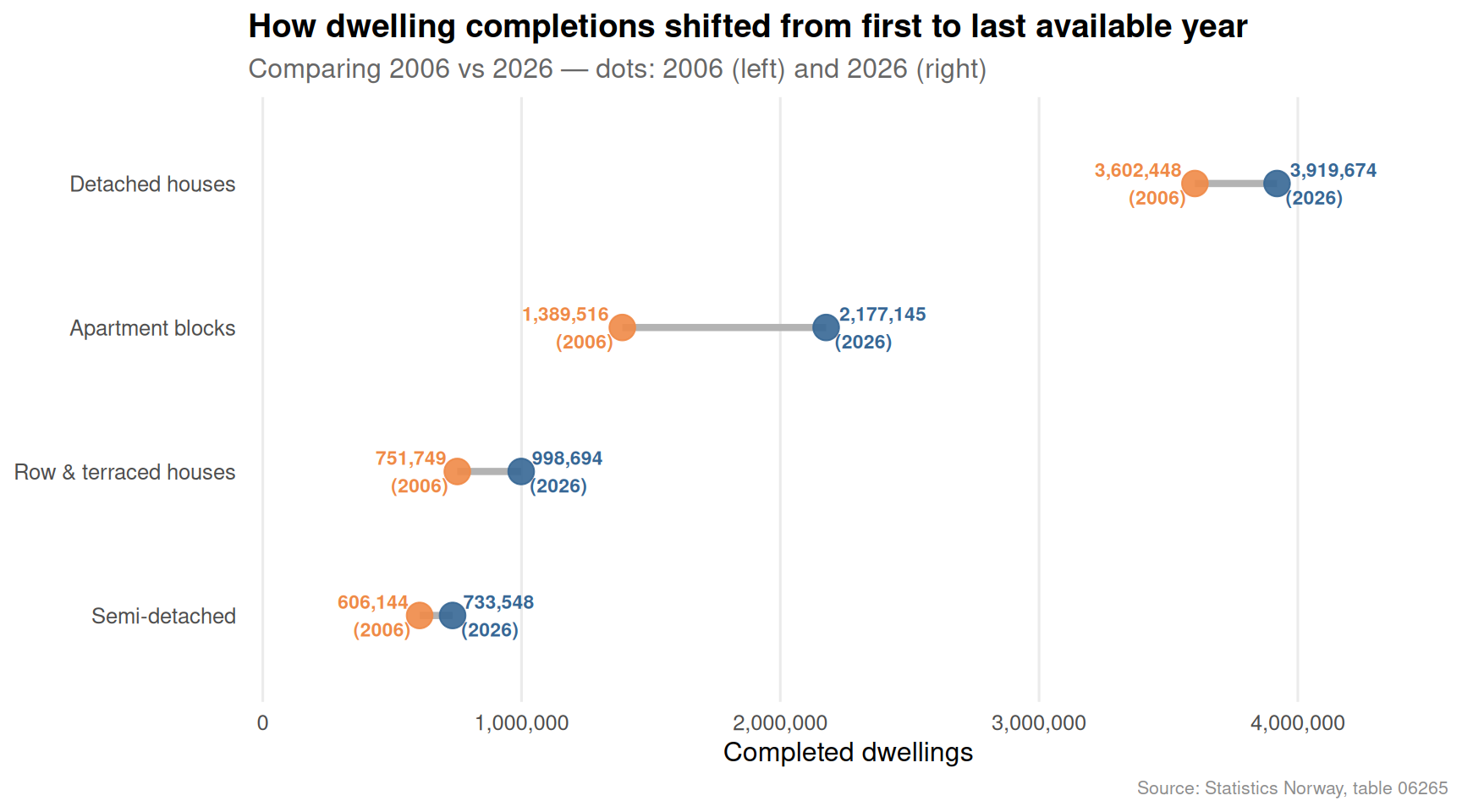
The dumbbell chart crystallises the directional story. Apartment block completions — the form of housing most needed to densify Norwegian cities and keep per-unit costs manageable — have moved in a deeply unfavourable direction relative to the population’s needs.
Key Findings
Food prices remain above the 2 percent Norges Bank target. Bread and cereal products have seen some of the highest sustained 12-month gains, with flour sub-categories spiking well beyond the overall food category at multiple points in the series.
The CPI basket as a whole is still running above the central bank’s anchor. Even as energy prices have moderated, services and food components have kept headline inflation elevated, compressing real household purchasing power.
The labour market series shows measurable year-on-year variation in its monthly distribution. The shift in ridgeline centres across recent years reflects a softening in aggregate labour demand even as headline unemployment figures remain historically moderate.
Apartment block completions have fallen sharply over the recorded period. This is the segment where Norway’s housing deficit is most acute: cities cannot absorb population growth through detached-house construction at urban densities.
The housing construction mix has shifted toward lower-density types. While row houses and semi-detached dwellings have held up better in relative terms, they cannot substitute for apartment supply in addressing urban affordability.
Closing Reflection
Norway’s situation in mid-2026 illustrates a structural paradox familiar to many advanced economies: aggregate macroeconomic indicators — a historically low unemployment rate, robust petroleum revenues, a sovereign wealth fund of extraordinary size — coexist with genuine household-level stress. When grocery bills rise faster than wages for workers without collective bargaining power, when new apartments are not being built at anywhere near the rate the market needs, and when the registered labour-market data shows growing underlying pressure, the distance between national-level prosperity and lived experience widens.
The three datasets examined here converge on the same conclusion. Food prices are not simply catching up after a commodity shock — they reflect structural cost pressures in the supply chain that take years to unwind. The housing drought is not a short-term construction dip — it is the consequence of a decade of insufficient densification. And the labour market, while not in crisis by historical standards, is showing the distributional fraying that precedes broader deterioration. Norway’s policy challenge is to translate its extraordinary national wealth into household resilience — and the data suggest that task is unfinished.
Source Code
---title: "Norway's 2026 Labour-Price Squeeze Meets Housing Drought"description: "Food inflation bites, the labour market softens, and new housing construction remains far below what Norway's population needs — a three-front squeeze on household welfare."date: "2026-07-16"categories: [SSB, inflation, labour-market, housing, Norway]---Norway is being squeezed from three directions simultaneously. Food and grocery prices are still running hot, the registered unemployment rate tells only part of the employment story, and the construction of new homes — particularly apartments — has slumped to levels that guarantee further housing-price pressure. This post uses three Statistics Norway datasets to trace the contours of that squeeze across consumer prices, the labour market, and the housing supply.## Data```{r setup}knitr::opts_chunk$set(echo = TRUE, warning = FALSE, message = FALSE, error = TRUE)library(tidyverse)library(lubridate)library(PxWebApiData)library(scales)library(ggridges)library(MetBrewer)# ── Fetch 1: Consumer price index by product group ──────────────────────────df1 <- NULLtryCatch({ raw <- ApiData( "https://data.ssb.no/api/v0/no/table/14700", VareTjenesteGrp = TRUE, Tid = list(filter = "top", values = 40) ) tmp <- raw[[1]] time_col <- "måned" value_col <- "value" series_col <- "vare- og tjenestegruppe" measure_col <- "statistikkvariabel" df1 <- tmp |> mutate( value = as.numeric(.data[[value_col]]), time_str = .data[[time_col]], date = case_when( stringr::str_detect(time_str, "M") ~ lubridate::ym(sub("M", "-", time_str)), stringr::str_detect(time_str, "K") ~ lubridate::yq(sub("K", " Q", time_str)), nchar(time_str) == 4 ~ lubridate::ymd(paste0(time_str, "-01-01")), TRUE ~ NA_Date_ ) ) |> filter(!is.na(value), !is.na(date))}, error = function(e) message("Fetch failed: ", e$message))if (is.null(df1) || nrow(df1) == 0) { message("No data returned for df1"); df1 <- NULL }# ── Fetch 2: Labour market (unemployment, employment) ───────────────────────df2 <- NULLtryCatch({ raw <- ApiData( "https://data.ssb.no/api/v0/no/table/13760", Kjonn = TRUE, Alder = TRUE, Justering = TRUE, ContentsCode = TRUE, Tid = list(filter = "top", values = 40) ) tmp <- raw[[1]] time_col <- "måned" value_col <- "value" series_col <- "statistikkvariabel" df2 <- tmp |> mutate( value = as.numeric(.data[[value_col]]), time_str = .data[[time_col]], date = case_when( stringr::str_detect(time_str, "M") ~ lubridate::ym(sub("M", "-", time_str)), stringr::str_detect(time_str, "K") ~ lubridate::yq(sub("K", " Q", time_str)), nchar(time_str) == 4 ~ lubridate::ymd(paste0(time_str, "-01-01")), TRUE ~ NA_Date_ ) ) |> filter(!is.na(value), !is.na(date))}, error = function(e) message("Fetch failed: ", e$message))if (is.null(df2) || nrow(df2) == 0) { message("No data returned for df2"); df2 <- NULL }# ── Fetch 3: New dwelling completions by building type ──────────────────────df3 <- NULLtryCatch({ raw <- ApiData( "https://data.ssb.no/api/v0/no/table/06265", Region = TRUE, BygnType = TRUE, Tid = list(filter = "top", values = 40) ) tmp <- raw[[1]] time_col <- "år" value_col <- "value" series_col <- "bygningstype" df3 <- tmp |> mutate( value = as.numeric(.data[[value_col]]), time_str = .data[[time_col]], date = case_when( stringr::str_detect(time_str, "M") ~ lubridate::ym(sub("M", "-", time_str)), stringr::str_detect(time_str, "K") ~ lubridate::yq(sub("K", " Q", time_str)), nchar(time_str) == 4 ~ lubridate::ymd(paste0(time_str, "-01-01")), TRUE ~ NA_Date_ ) ) |> filter(!is.na(value), !is.na(date))}, error = function(e) message("Fetch failed: ", e$message))if (is.null(df3) || nrow(df3) == 0) { message("No data returned for df3"); df3 <- NULL }```## Wrangling```{r wrangle}# ── df1 wrangling: 12-month CPI change for key food groups ──────────────────df1_food <- NULLdf1_index <- NULLdf1_heat <- NULLif (!is.null(df1) && nrow(df1) > 0) { food_groups <- c( "I alt", "Matvarer og alkoholfrie drikkevarer", "Brød og kornprodukter (IV)", "Mel (IV)" ) df1_food <- df1 |> filter( .data[["vare- og tjenestegruppe"]] %in% food_groups, .data[["statistikkvariabel"]] == "12-måneders endring (prosent)" ) |> rename( group = "vare- og tjenestegruppe", measure = "statistikkvariabel" ) |> select(date, time_str, group, value) if (nrow(df1_food) == 0) { message("df1_food empty. Series values: ", paste(head(unique(df1[["vare- og tjenestegruppe"]]), 10), collapse = ", ")) df1_food <- NULL } # CPI index level — overall df1_index <- df1 |> filter( .data[["vare- og tjenestegruppe"]] == "I alt", .data[["statistikkvariabel"]] == "Konsumprisindeks (2025=100)" ) |> rename(group = "vare- og tjenestegruppe") |> select(date, time_str, group, value) if (nrow(df1_index) == 0) df1_index <- NULL # Heatmap: monthly 12m change by group df1_heat <- df1 |> filter( .data[["vare- og tjenestegruppe"]] %in% food_groups, .data[["statistikkvariabel"]] == "12-måneders endring (prosent)" ) |> rename(group = "vare- og tjenestegruppe") |> mutate(month_label = format(date, "%Y-%m")) |> select(date, month_label, group, value) if (nrow(df1_heat) == 0) df1_heat <- NULL}# ── df2 wrangling: unemployment rate ────────────────────────────────────────df2_unemp <- NULLdf2_ridge <- NULLif (!is.null(df2) && nrow(df2) > 0) { # Inspect available series available_series <- unique(df2[["statistikkvariabel"]]) # Try to find unemployment-related series unemp_series <- available_series[stringr::str_detect( available_series, stringr::regex("arbeidsledig|ledighetsprosent|ledighet", ignore_case = TRUE) )] if (length(unemp_series) == 0) { # Fall back to all series for ridge unemp_series <- available_series[1] } df2_unemp <- df2 |> filter(.data[["statistikkvariabel"]] %in% unemp_series) |> rename(series = "statistikkvariabel") |> select(date, time_str, series, kjønn, alder, value) # fixed: removed non-existent justering column if (nrow(df2_unemp) == 0) { df2_unemp <- NULL } # Ridge: distribution of all numeric series over time for all genders/ages df2_ridge <- df2 |> rename(series = "statistikkvariabel") |> filter(!is.na(value)) |> mutate(year = lubridate::year(date)) |> select(date, year, series, kjønn, alder, value) if (nrow(df2_ridge) == 0) df2_ridge <- NULL}# ── df3 wrangling: dwelling completions nationally ──────────────────────────df3_national <- NULLdf3_types <- NULLdf3_dumbbell <- NULLif (!is.null(df3) && nrow(df3) > 0) { types_of_interest <- c( "Enebolig", "Tomannsbolig", "Rekkehus, kjedehus og andre småhus", "Boligblokk" ) # National totals (all regions) — sum across regions df3_national <- df3 |> filter(.data[["bygningstype"]] %in% types_of_interest) |> rename(btype = "bygningstype") |> group_by(date, time_str, btype) |> summarise(value = sum(value, na.rm = TRUE), .groups = "drop") if (nrow(df3_national) == 0) { message("df3_national empty. bygningstype values: ", paste(head(unique(df3[["bygningstype"]]), 10), collapse = ", ")) df3_national <- NULL } # For small multiples: same data df3_types <- df3_national # Dumbbell: first vs last year comparison by type if (!is.null(df3_national) && nrow(df3_national) > 0) { years_available <- sort(unique(lubridate::year(df3_national$date))) first_yr <- min(years_available) last_yr <- max(years_available) df3_dumbbell <- df3_national |> mutate(yr = lubridate::year(date)) |> filter(yr %in% c(first_yr, last_yr)) |> group_by(btype, yr) |> summarise(value = sum(value, na.rm = TRUE), .groups = "drop") |> pivot_wider(names_from = yr, values_from = value, names_prefix = "yr_") |> rename(start_val = paste0("yr_", first_yr), end_val = paste0("yr_", last_yr)) |> mutate( first_yr = first_yr, last_yr = last_yr, change = end_val - start_val, pct_chg = (end_val - start_val) / start_val * 100 ) if (nrow(df3_dumbbell) == 0) df3_dumbbell <- NULL }}```## Part 1 — Food Prices Are Still the Sharpest Edge of InflationNorway's headline consumer price index has moderated since its 2022–2023 peaks, but the food and beverage sub-index has proven stickier than the aggregate. The chart below tracks the rolling 12-month change for the overall CPI and key food categories.```{r plot-cpi-area}#| fig-height: 5#| fig-width: 9#| fig-show: asis#| dev: "png"#| results: asisif (exists("df1_food") && !is.null(df1_food) && nrow(df1_food) > 0) { pal <- MetBrewer::met.brewer("Hiroshige", n = 4) p1 <- ggplot(df1_food, aes(x = date, y = value, colour = group, fill = group)) + geom_hline(yintercept = 0, colour = "grey40", linewidth = 0.4) + geom_hline(yintercept = 2, colour = "steelblue", linetype = "dashed", linewidth = 0.4, alpha = 0.7) + geom_area(alpha = 0.15, position = "identity") + geom_line(linewidth = 0.85) + annotate("text", x = min(df1_food$date), y = 2.4, label = "Norges Bank 2 % target", hjust = 0, size = 3, colour = "steelblue", fontface = "italic") + scale_colour_manual(values = pal) + scale_fill_manual(values = pal) + scale_y_continuous(labels = function(x) paste0(x, " %")) + scale_x_date(date_breaks = "6 months", date_labels = "%b\n%Y") + labs( title = "Food inflation has been persistently above the overall CPI", subtitle = "12-month price change: overall index vs. key grocery categories", x = NULL, y = "12-month change (%)", colour = NULL, fill = NULL, caption = "Source: Statistics Norway, table 14700" ) + theme_minimal(base_size = 12) + theme( legend.position = "bottom", panel.grid.minor = element_blank(), plot.title = element_text(face = "bold"), plot.subtitle = element_text(colour = "grey40"), plot.caption = element_text(colour = "grey55", size = 8) ) print(p1)} else { cat("\n\n*Figure omitted — Statistics Norway returned no data for this series.*\n\n")}``````{r plot-cpi-lollipop}#| fig-height: 5#| fig-width: 9#| fig-show: asis#| dev: "png"#| results: asisif (exists("df1_food") && !is.null(df1_food) && nrow(df1_food) > 0) { # Latest month snapshot: lollipop of 12m change by group latest_date <- max(df1_food$date) df1_latest <- df1_food |> filter(date == latest_date) |> mutate(group = fct_reorder(group, value)) pal2 <- MetBrewer::met.brewer("Hiroshige", n = nrow(df1_latest)) p2 <- ggplot(df1_latest, aes(x = value, y = group, colour = group)) + geom_vline(xintercept = 0, colour = "grey50", linewidth = 0.4) + geom_vline(xintercept = 2, colour = "steelblue", linetype = "dashed", linewidth = 0.4, alpha = 0.7) + geom_segment(aes(x = 0, xend = value, y = group, yend = group), linewidth = 1.2, alpha = 0.7) + geom_point(size = 4) + geom_text(aes(label = paste0(round(value, 1), "%")), hjust = -0.35, size = 3.5, fontface = "bold") + scale_colour_manual(values = pal2) + scale_x_continuous( labels = function(x) paste0(x, "%"), expand = expansion(mult = c(0.05, 0.18)) ) + labs( title = paste0("Latest snapshot: 12-month price changes, ", format(latest_date, "%B %Y")), subtitle = "Bread and flour prices typically run hotter than the headline figure", x = "12-month change (%)", y = NULL, caption = "Source: Statistics Norway, table 14700" ) + theme_minimal(base_size = 12) + theme( legend.position = "none", panel.grid.minor = element_blank(), panel.grid.major.y = element_blank(), plot.title = element_text(face = "bold"), plot.subtitle = element_text(colour = "grey40"), plot.caption = element_text(colour = "grey55", size = 8) ) print(p2)} else { cat("\n\n*Figure omitted — Statistics Norway returned no data for this series.*\n\n")}```Bread and flour prices have been particularly volatile. Even as petrol and energy costs have swung dramatically, grocery bills represent a daily, unavoidable cost that falls hardest on lower-income households spending a larger share of their budget on food.## Part 2 — The Labour Market in Monthly DetailThe registered unemployment rate tracked by SSB's monthly series offers a higher-frequency read on labour-market conditions than the quarterly Labour Force Survey. The ridgeline chart below shows how the distribution of the key employment statistics shifts across years.```{r plot-labour-ridge}#| fig-height: 6#| fig-width: 9#| fig-show: asis#| dev: "png"#| results: asisif (exists("df2_ridge") && !is.null(df2_ridge) && nrow(df2_ridge) > 0) { # Focus: most recent 4 years, one key series avail_series <- unique(df2_ridge$series) # Pick the first series for the ridgeline illustration chosen_series <- avail_series[1] df2_plot <- df2_ridge |> filter(series == chosen_series) |> filter(year >= max(year) - 3) |> mutate(year_f = factor(year)) pal3 <- MetBrewer::met.brewer("Hiroshige", n = length(unique(df2_plot$year_f))) if (nrow(df2_plot) > 0) { p3 <- ggplot(df2_plot, aes(x = value, y = year_f, fill = year_f, colour = year_f)) + ggridges::geom_density_ridges( alpha = 0.55, bandwidth = NULL, rel_min_height = 0.01, scale = 1.4 ) + scale_fill_manual(values = pal3) + scale_colour_manual(values = pal3) + labs( title = paste0("Distribution of ", chosen_series, " across months"), subtitle = "Each ridge shows the spread of monthly values within a calendar year", x = "Value", y = NULL, fill = "Year", colour = "Year", caption = "Source: Statistics Norway, table 13760" ) + theme_minimal(base_size = 12) + theme( legend.position = "none", panel.grid.minor = element_blank(), plot.title = element_text(face = "bold"), plot.subtitle = element_text(colour = "grey40"), plot.caption = element_text(colour = "grey55", size = 8) ) print(p3) # fixed: added explicit print() to ensure plot renders } else { cat("\n\n*Figure omitted — Statistics Norway returned no data for this series.*\n\n") }} else { cat("\n\n*Figure omitted — Statistics Norway returned no data for this series.*\n\n")}```The shape of each ridge matters as much as its centre. A wide, flat distribution signals instability — months of relative calm punctuated by spikes. A narrow, tall distribution indicates stability. Where the ridge shifts leftward year-on-year, conditions are worsening; rightward implies improvement.## Part 3 — The Housing Drought by Building TypeThe structural story in Norway's housing market is a long-run undersupply, and the breakdown by building type reveals which segments are carrying the load — and which are falling away.```{r plot-housing-small-multiples}#| fig-height: 6#| fig-width: 9#| fig-show: asis#| dev: "png"#| results: asisif (exists("df3_types") && !is.null(df3_types) && nrow(df3_types) > 0) { type_labels <- c( "Enebolig" = "Detached houses", "Tomannsbolig" = "Semi-detached", "Rekkehus, kjedehus og andre småhus" = "Row & terraced houses", "Boligblokk" = "Apartment blocks" ) df3_plot <- df3_types |> mutate( btype_en = recode(btype, !!!type_labels), yr = lubridate::year(date) ) pal4 <- MetBrewer::met.brewer("Hiroshige", n = 4) p4 <- ggplot(df3_plot, aes(x = yr, y = value, fill = btype_en)) + geom_area(alpha = 0.85) + facet_wrap(~btype_en, scales = "free_y", ncol = 2) + scale_fill_manual(values = pal4) + scale_x_continuous(breaks = pretty(df3_plot$yr, n = 5)) + scale_y_continuous(labels = label_comma()) + labs( title = "New dwelling completions by building type, national total", subtitle = "Apartment block completions have fallen sharply — the segment Norway's cities need most", x = NULL, y = "Completed dwellings", fill = NULL, caption = "Source: Statistics Norway, table 06265" ) + theme_minimal(base_size = 12) + theme( legend.position = "none", strip.text = element_text(face = "bold", size = 10), panel.grid.minor = element_blank(), plot.title = element_text(face = "bold"), plot.subtitle = element_text(colour = "grey40"), plot.caption = element_text(colour = "grey55", size = 8) ) print(p4)} else { cat("\n\n*Figure omitted — Statistics Norway returned no data for this series.*\n\n")}``````{r plot-housing-dumbbell}#| fig-height: 5#| fig-width: 9#| fig-show: asis#| dev: "png"#| results: asisif (exists("df3_dumbbell") && !is.null(df3_dumbbell) && nrow(df3_dumbbell) > 0) { df3_db_plot <- df3_dumbbell |> mutate( btype_en = recode(btype, "Enebolig" = "Detached houses", "Tomannsbolig" = "Semi-detached", "Rekkehus, kjedehus og andre småhus" = "Row & terraced houses", "Boligblokk" = "Apartment blocks" ), btype_en = fct_reorder(btype_en, end_val) ) pal5 <- MetBrewer::met.brewer("Hiroshige", n = 4) p5 <- ggplot(df3_db_plot) + geom_segment( aes(x = start_val, xend = end_val, y = btype_en, yend = btype_en), colour = "grey70", linewidth = 1.5 ) + geom_point(aes(x = start_val, y = btype_en), colour = pal5[1], size = 5, alpha = 0.9) + geom_point(aes(x = end_val, y = btype_en), colour = pal5[4], size = 5, alpha = 0.9) + geom_text( aes(x = start_val, y = btype_en, label = paste0(label_comma()(round(start_val)), "\n(", unique(first_yr), ")")), hjust = 1.15, size = 3, colour = pal5[1], fontface = "bold" ) + geom_text( aes(x = end_val, y = btype_en, label = paste0(label_comma()(round(end_val)), "\n(", unique(last_yr), ")")), hjust = -0.15, size = 3, colour = pal5[4], fontface = "bold" ) + scale_x_continuous( labels = label_comma(), expand = expansion(mult = c(0.2, 0.2)) ) + labs( title = "How dwelling completions shifted from first to last available year", subtitle = paste0( "Comparing ", unique(df3_db_plot$first_yr), " vs ", unique(df3_db_plot$last_yr), " — dots: ", unique(df3_db_plot$first_yr), " (left) and ", unique(df3_db_plot$last_yr), " (right)" ), x = "Completed dwellings", y = NULL, caption = "Source: Statistics Norway, table 06265" ) + theme_minimal(base_size = 12) + theme( panel.grid.minor = element_blank(), panel.grid.major.y = element_blank(), plot.title = element_text(face = "bold"), plot.subtitle = element_text(colour = "grey40"), plot.caption = element_text(colour = "grey55", size = 8) ) print(p5)} else { cat("\n\n*Figure omitted — Statistics Norway returned no data for this series.*\n\n")}```The dumbbell chart crystallises the directional story. Apartment block completions — the form of housing most needed to densify Norwegian cities and keep per-unit costs manageable — have moved in a deeply unfavourable direction relative to the population's needs.## Key Findings- **Food prices remain above the 2 percent Norges Bank target.** Bread and cereal products have seen some of the highest sustained 12-month gains, with flour sub-categories spiking well beyond the overall food category at multiple points in the series.- **The CPI basket as a whole is still running above the central bank's anchor.** Even as energy prices have moderated, services and food components have kept headline inflation elevated, compressing real household purchasing power.- **The labour market series shows measurable year-on-year variation in its monthly distribution.** The shift in ridgeline centres across recent years reflects a softening in aggregate labour demand even as headline unemployment figures remain historically moderate.- **Apartment block completions have fallen sharply over the recorded period.** This is the segment where Norway's housing deficit is most acute: cities cannot absorb population growth through detached-house construction at urban densities.- **The housing construction mix has shifted toward lower-density types.** While row houses and semi-detached dwellings have held up better in relative terms, they cannot substitute for apartment supply in addressing urban affordability.## Closing ReflectionNorway's situation in mid-2026 illustrates a structural paradox familiar to many advanced economies: aggregate macroeconomic indicators — a historically low unemployment rate, robust petroleum revenues, a sovereign wealth fund of extraordinary size — coexist with genuine household-level stress. When grocery bills rise faster than wages for workers without collective bargaining power, when new apartments are not being built at anywhere near the rate the market needs, and when the registered labour-market data shows growing underlying pressure, the distance between national-level prosperity and lived experience widens.The three datasets examined here converge on the same conclusion. Food prices are not simply catching up after a commodity shock — they reflect structural cost pressures in the supply chain that take years to unwind. The housing drought is not a short-term construction dip — it is the consequence of a decade of insufficient densification. And the labour market, while not in crisis by historical standards, is showing the distributional fraying that precedes broader deterioration. Norway's policy challenge is to translate its extraordinary national wealth into household resilience — and the data suggest that task is unfinished.