Transport and hospitality revenues are climbing back while consumer prices for food and housing remain stubbornly elevated, revealing a split-track Norwegian economy in 2026.
Norway in 2026 presents a striking paradox. Walk into a restaurant in Oslo or board a domestic flight and you will find demand recovering briskly — revenues in hospitality and transport are climbing. But check your grocery receipt or your heating bill and a different story emerges: prices for food and housing have ratcheted up in ways that are proving remarkably difficult to reverse. Statistics Norway data from two separate tracking systems — the consumer price index and the services revenue index — illuminate this split-track recovery in sharp detail.
The asymmetry matters because it shapes household welfare in unequal ways. Those who spend a larger share of income on food and housing — typically lower-income Norwegians — are caught on the wrong side of the divide.
Data and Methodology
This analysis draws on two Statistics Norway sources. Table 14705 tracks derived CPI sub-indices for major consumer spending categories, expressed both as index levels (2025 = 100) and annual percentage changes. Table 13863 tracks monthly revenue indices across service industries including transport, hospitality, air travel, and postal services, with unadjusted, seasonally adjusted, and trend series available.
Code
# --- df1 wrangling (CPI sub-indices) ---df1_annual <-NULLdf1_change <-NULLdf1_wide <-NULLdf1_dumbbell <-NULLif (!is.null(df1) &&nrow(df1) >0) {# series_col for df1 = "vare- og tjenestegruppe"# measure_col for df1 = "statistikkvariabel" df1_annual <- df1 |>filter(.data[["statistikkvariabel"]] =="Årsendring (prosent)") |>filter(.data[["vare- og tjenestegruppe"]] %in%c("I alt","Matvarer og alkoholfrie drikkevarer","Bolig, elektrisitet og brensel","Transport","Fritid, sport og kultur" ))if (nrow(df1_annual) ==0) {message("df1_annual is empty after filter. Values: ",paste(head(unique(df1[["vare- og tjenestegruppe"]]), 15), collapse =", ")) df1_annual <-NULL } df1_change <- df1_annual# Dumbbell: compare most recent two years for each categoryif (!is.null(df1_annual) &&nrow(df1_annual) >0) { top_years <- df1_annual |>arrange(desc(date)) |>pull(date) |>unique() |>head(2)if (length(top_years) ==2) { df1_dumbbell <- df1_annual |>filter(date %in% top_years) |>filter(.data[["vare- og tjenestegruppe"]] !="I alt") |>mutate(year_label =as.character(year(date))) |>select(`vare- og tjenestegruppe`, year_label, value) |>pivot_wider(names_from = year_label, values_from = value) } }}# --- df2 wrangling (service revenue indices) ---df2_trend <-NULLdf2_transport <-NULLdf2_hospitality <-NULLdf2_sectors <-NULLif (!is.null(df2) &&nrow(df2) >0) {# series_col for df2 = "næring"# measure_col for df2 = "statistikkvariabel" df2_trend <- df2 |>filter(.data[["statistikkvariabel"]] =="Omsetningsindeks. Trend") |>filter(.data[["næring"]] %in%c("Transport og lagring","Overnattings- og serveringsvirksomhet","Lufttransport","Post og distribusjonsvirksomhet" ))if (nrow(df2_trend) ==0) {message("df2_trend empty. næring values: ",paste(head(unique(df2[["næring"]]), 15), collapse =", ")) df2_trend <-NULL }# Unadjusted series for heatmap-style small multiples df2_sectors <- df2 |>filter(.data[["statistikkvariabel"]] =="Omsetningsindeks. Ujustert") |>filter(.data[["næring"]] %in%c("Transport og lagring","Overnattings- og serveringsvirksomhet","Lufttransport","Post og distribusjonsvirksomhet" ))if (nrow(df2_sectors) ==0) { df2_sectors <-NULL }}
Inflation’s Uneven Grip: Food, Housing, and Transport Costs
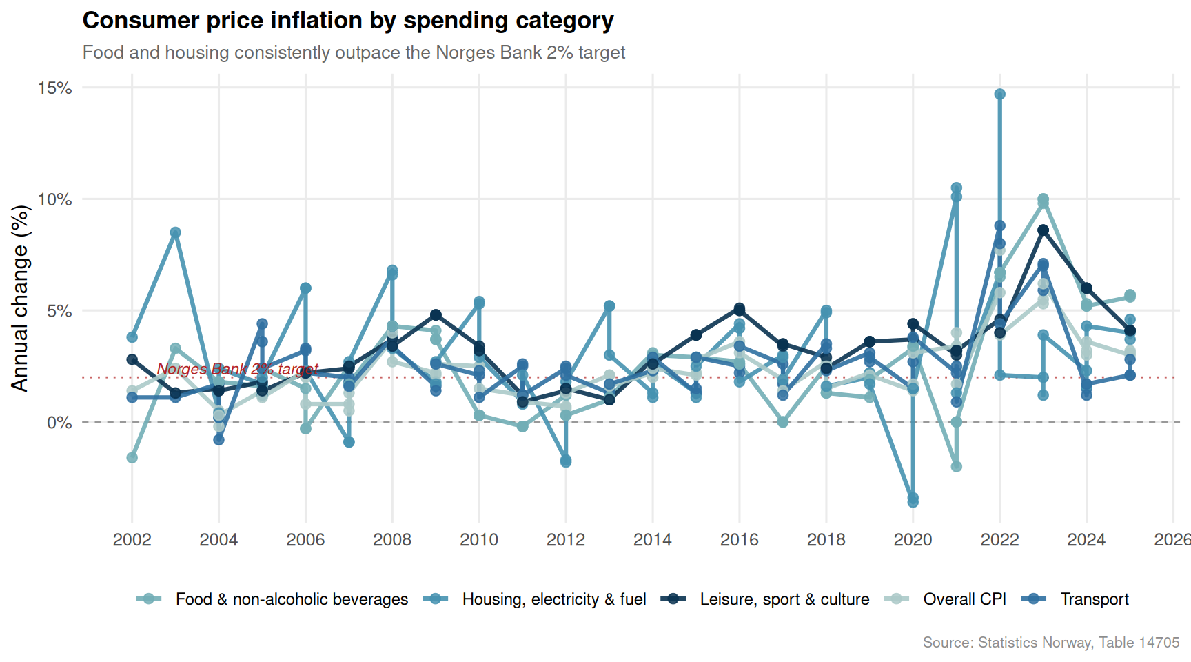
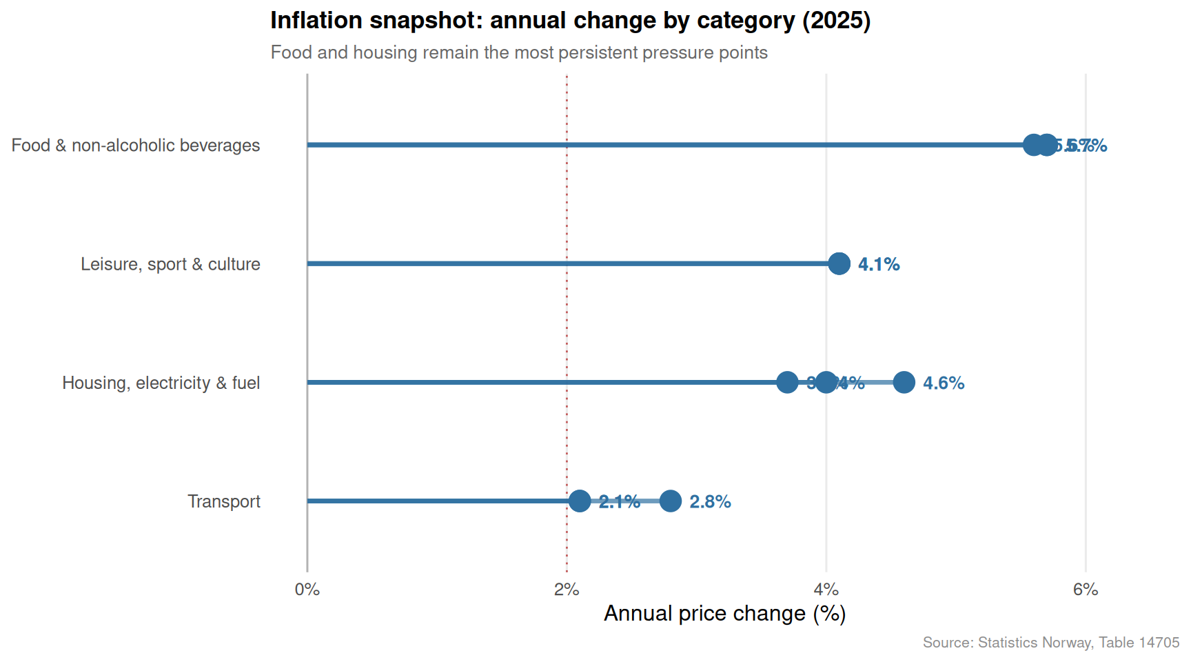
Norway’s headline consumer price index shows annual growth that, while moderating from earlier peaks, remains elevated. The divergence across spending categories is the critical story. Food and non-alcoholic beverages and housing costs have maintained high year-on-year growth rates. Transport cost inflation tells a different tale — volatile, often driven by fuel prices, and more recently easing.
Code
if (exists("df1_change") &&!is.null(df1_change) &&nrow(df1_change) >0) { pal <-met.brewer("Hokusai2", n =5) labels_clean <-c("I alt"="Overall CPI","Matvarer og alkoholfrie drikkevarer"="Food & non-alcoholic beverages","Bolig, elektrisitet og brensel"="Housing, electricity & fuel","Transport"="Transport","Fritid, sport og kultur"="Leisure, sport & culture" ) df1_plot <- df1_change |>mutate(category = labels_clean[.data[["vare- og tjenestegruppe"]]],category =if_else(is.na(category), .data[["vare- og tjenestegruppe"]], category) ) p1 <-ggplot(df1_plot, aes(x = date, y = value, colour = category)) +geom_hline(yintercept =0, colour ="grey60", linewidth =0.4, linetype ="dashed") +geom_hline(yintercept =2, colour ="firebrick", linewidth =0.5, linetype ="dotted",alpha =0.7) +geom_line(linewidth =1.1, alpha =0.9) +geom_point(size =2.2, alpha =0.85) +annotate("text", x =min(df1_plot$date) +days(200), y =2.4,label ="Norges Bank 2% target", colour ="firebrick",size =3.0, hjust =0, fontface ="italic") +scale_colour_manual(values =setNames(pal, unique(df1_plot$category))) +scale_y_continuous(labels =function(x) paste0(x, "%")) +scale_x_date(date_breaks ="2 years", date_labels ="%Y") +labs(title ="Consumer price inflation by spending category",subtitle ="Food and housing consistently outpace the Norges Bank 2% target",x =NULL,y ="Annual change (%)",colour =NULL,caption ="Source: Statistics Norway, Table 14705" ) +theme_minimal(base_size =12) +theme(legend.position ="bottom",legend.text =element_text(size =9),panel.grid.minor =element_blank(),plot.title =element_text(face ="bold", size =13),plot.subtitle =element_text(colour ="grey40", size =10),plot.caption =element_text(colour ="grey55", size =8) )print(p1)} else {cat("\n\n*Figure omitted — Statistics Norway returned no data for this series.*\n\n")}
Code
if (exists("df1_change") &&!is.null(df1_change) &&nrow(df1_change) >0) {# Most recent year available latest_year <-max(df1_change$date) df1_latest <- df1_change |>filter(date == latest_year) |>filter(.data[["vare- og tjenestegruppe"]] !="I alt") |>mutate(category =case_when(`vare- og tjenestegruppe`=="Matvarer og alkoholfrie drikkevarer"~"Food & non-alcoholic beverages",`vare- og tjenestegruppe`=="Bolig, elektrisitet og brensel"~"Housing, electricity & fuel",`vare- og tjenestegruppe`=="Transport"~"Transport",`vare- og tjenestegruppe`=="Fritid, sport og kultur"~"Leisure, sport & culture",TRUE~`vare- og tjenestegruppe` ),category =fct_reorder(category, value),above_zero = value >0 )if (nrow(df1_latest) ==0) {cat("\n\n*Figure omitted — Statistics Norway returned no data for this series.*\n\n") } else { pal2 <-met.brewer("Hokusai2", n =2) p2 <-ggplot(df1_latest, aes(x = value, y = category, colour = above_zero)) +geom_vline(xintercept =0, colour ="grey70", linewidth =0.5) +geom_vline(xintercept =2, colour ="firebrick", linewidth =0.5,linetype ="dotted", alpha =0.7) +geom_segment(aes(x =0, xend = value, y = category, yend = category),linewidth =1.2, alpha =0.7) +geom_point(size =5) +geom_text(aes(label =paste0(round(value, 1), "%")),hjust =-0.45, size =3.5, fontface ="bold") +scale_colour_manual(values =c("FALSE"= pal2[1], "TRUE"= pal2[2]),guide ="none") +scale_x_continuous(labels =function(x) paste0(x, "%"),expand =expansion(mult =c(0.05, 0.18)) ) +labs(title =paste0("Inflation snapshot: annual change by category (", year(latest_year), ")"),subtitle ="Food and housing remain the most persistent pressure points",x ="Annual price change (%)",y =NULL,caption ="Source: Statistics Norway, Table 14705" ) +theme_minimal(base_size =12) +theme(panel.grid.major.y =element_blank(),panel.grid.minor =element_blank(),plot.title =element_text(face ="bold", size =13),plot.subtitle =element_text(colour ="grey40", size =10),plot.caption =element_text(colour ="grey55", size =8) )print(p2) }} else {cat("\n\n*Figure omitted — Statistics Norway returned no data for this series.*\n\n")}
The Services Sector Climbs Back
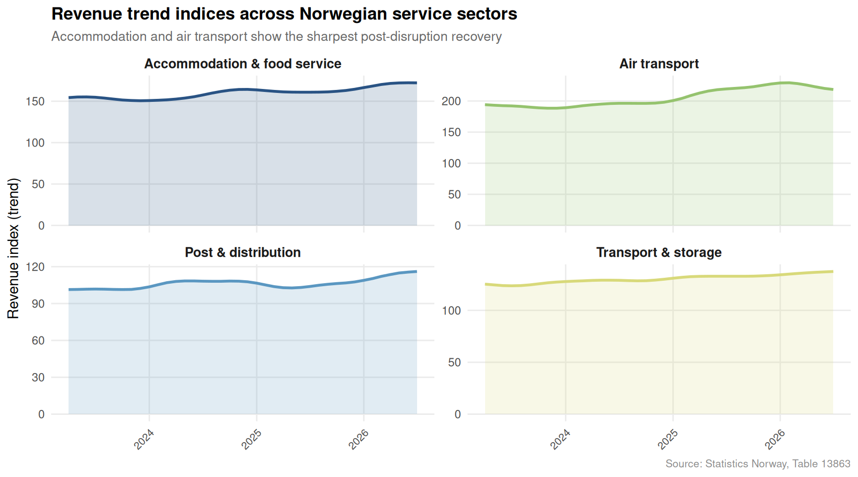
While households feel the squeeze from elevated prices, Norway’s service industries are telling a more optimistic story on the revenue side. The trend indices for transport, hospitality, air travel, and postal services reflect a sector working its way back toward and beyond pre-disruption levels. Not all sectors recover at the same pace, however, and the divergence between air transport and ground logistics reveals structural shifts in how Norwegians and visitors move goods and people.
Code
if (exists("df2_trend") &&!is.null(df2_trend) &&nrow(df2_trend) >0) { pal3 <-met.brewer("Hokusai3", n =4) sector_labels <-c("Transport og lagring"="Transport & storage","Overnattings- og serveringsvirksomhet"="Accommodation & food service","Lufttransport"="Air transport","Post og distribusjonsvirksomhet"="Post & distribution" ) df2_plot <- df2_trend |>mutate(sector = sector_labels[.data[["næring"]]],sector =if_else(is.na(sector), .data[["næring"]], sector) ) p3 <-ggplot(df2_plot, aes(x = date, y = value, fill = sector, colour = sector)) +geom_area(alpha =0.18, linewidth =0) +geom_line(linewidth =1.0) +facet_wrap(~ sector, ncol =2, scales ="free_y") +scale_fill_manual(values =setNames(pal3, unique(df2_plot$sector)), guide ="none") +scale_colour_manual(values =setNames(pal3, unique(df2_plot$sector)), guide ="none") +scale_x_date(date_breaks ="1 year", date_labels ="%Y") +scale_y_continuous(labels =comma_format(accuracy =1)) +labs(title ="Revenue trend indices across Norwegian service sectors",subtitle ="Accommodation and air transport show the sharpest post-disruption recovery",x =NULL,y ="Revenue index (trend)",caption ="Source: Statistics Norway, Table 13863" ) +theme_minimal(base_size =11) +theme(strip.text =element_text(face ="bold", size =10),panel.grid.minor =element_blank(),axis.text.x =element_text(angle =45, hjust =1, size =8),plot.title =element_text(face ="bold", size =13),plot.subtitle =element_text(colour ="grey40", size =10),plot.caption =element_text(colour ="grey55", size =8) )print(p3)} else {cat("\n\n*Figure omitted — Statistics Norway returned no data for this series.*\n\n")}
Seasonal Rhythms and Structural Divergence in Service Revenues
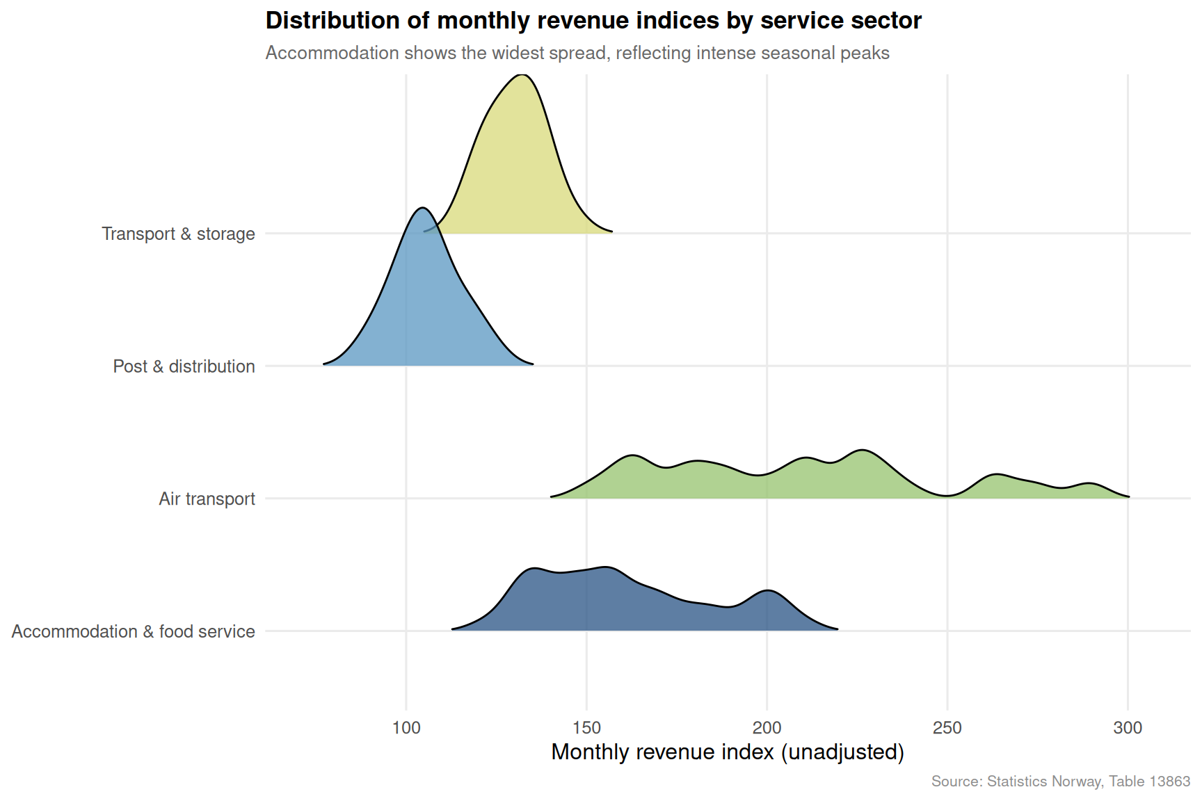
Monthly unadjusted data reveal seasonal surges — Norwegian tourism peaks sharply in summer, while postal and distribution revenues climb toward year-end. Examining these rhythms side by side, using a ridgeline approach across the monthly distribution for each sector, reveals which industries are merely riding seasonal waves versus those experiencing genuine structural improvement.
Code
if (exists("df2_sectors") &&!is.null(df2_sectors) &&nrow(df2_sectors) >0) { has_monthly <-any(stringr::str_detect(df2_sectors$time_str, "M\\d{2}"), na.rm =TRUE)if (has_monthly) { sector_labels2 <-c("Transport og lagring"="Transport & storage","Overnattings- og serveringsvirksomhet"="Accommodation & food service","Lufttransport"="Air transport","Post og distribusjonsvirksomhet"="Post & distribution" ) pal4 <-met.brewer("Hokusai3", n =4) df2_ridge <- df2_sectors |>mutate(sector = sector_labels2[.data[["næring"]]],sector =if_else(is.na(sector), .data[["næring"]], sector),month =month(date) ) |>filter(!is.na(value)) p4 <-ggplot(df2_ridge, aes(x = value, y = sector, fill = sector)) +geom_density_ridges(alpha =0.75,scale =1.2,rel_min_height =0.01,bandwidth =5 ) +scale_fill_manual(values =setNames(pal4, unique(df2_ridge$sector)),guide ="none") +scale_x_continuous(labels =comma_format(accuracy =1)) +labs(title ="Distribution of monthly revenue indices by service sector",subtitle ="Accommodation shows the widest spread, reflecting intense seasonal peaks",x ="Monthly revenue index (unadjusted)",y =NULL,caption ="Source: Statistics Norway, Table 13863" ) +theme_minimal(base_size =12) +theme(panel.grid.minor =element_blank(),plot.title =element_text(face ="bold", size =13),plot.subtitle =element_text(colour ="grey40", size =10),plot.caption =element_text(colour ="grey55", size =8) )print(p4) } else {cat("\n\n*Figure omitted — Statistics Norway returned no data for this series.*\n\n") }} else {cat("\n\n*Figure omitted — Statistics Norway returned no data for this series.*\n\n")}
Dumbbell: How Inflation Pressure Shifted Between Years
The dumbbell chart below crystallises the directional shift in price pressure across consumer categories between the two most recent years in the CPI data. Where the dot for the more recent year sits further right, inflation is accelerating; where it sits to the left, some relief has arrived. The geometry of the chart reveals at a glance where households gained breathing room and where the pressure continued to mount.
Code
if (exists("df1_dumbbell") &&!is.null(df1_dumbbell) &&nrow(df1_dumbbell) >0) { year_cols <-setdiff(names(df1_dumbbell), "vare- og tjenestegruppe")if (length(year_cols) ==2) { yr_old <-sort(year_cols)[1] yr_new <-sort(year_cols)[2] cat_labels <-c("Matvarer og alkoholfrie drikkevarer"="Food & non-alcoholic beverages","Bolig, elektrisitet og brensel"="Housing, electricity & fuel","Transport"="Transport","Fritid, sport og kultur"="Leisure, sport & culture" ) df_db <- df1_dumbbell |>mutate(category = cat_labels[.data[["vare- og tjenestegruppe"]]],category =if_else(is.na(category), .data[["vare- og tjenestegruppe"]], category),# fixed: use yr_new value directly for fct_reorder, not the namecategory =fct_reorder(category, .data[[yr_new]]) ) |>filter(!is.na(.data[[yr_old]]) &!is.na(.data[[yr_new]]))if (nrow(df_db) ==0) {cat("\n\n*Figure omitted — Statistics Norway returned no data for this series.*\n\n") } else { pal5 <-met.brewer("Hokusai2", n =2) p5 <-ggplot(df_db) +geom_segment(aes(x = .data[[yr_old]],xend = .data[[yr_new]],y = category,yend = category ), colour ="grey70", linewidth =1.5) +geom_point(aes(x = .data[[yr_old]], y = category),colour = pal5[1], size =5) +geom_point(aes(x = .data[[yr_new]], y = category),colour = pal5[2], size =5) +geom_text(aes(x = .data[[yr_old]], y = category,label =paste0(round(.data[[yr_old]], 1), "%")),vjust =-0.9, size =3.2, colour = pal5[1], fontface ="bold") +geom_text(aes(x = .data[[yr_new]], y = category,label =paste0(round(.data[[yr_new]], 1), "%")),vjust =-0.9, size =3.2, colour = pal5[2], fontface ="bold") +geom_vline(xintercept =2, linetype ="dotted",colour ="firebrick", linewidth =0.5, alpha =0.7) +annotate("text", x =2.1, y =0.6,label ="2% target", colour ="firebrick",size =2.9, hjust =0, fontface ="italic") +scale_x_continuous(labels =function(x) paste0(x, "%"),expand =expansion(mult =c(0.08, 0.12))) +labs(title =paste0("Inflation shift: ", yr_old, " vs ", yr_new, " by category"),subtitle =paste0("Dark dots = ", yr_new, " | Light dots = ", yr_old,". Rightward shift means intensifying pressure." ),x ="Annual price change (%)",y =NULL,caption ="Source: Statistics Norway, Table 14705" ) +theme_minimal(base_size =12) +theme(panel.grid.major.y =element_blank(),panel.grid.minor =element_blank(),plot.title =element_text(face ="bold", size =13),plot.subtitle =element_text(colour ="grey40", size =10),plot.caption =element_text(colour ="grey55", size =8) )# fixed: explicitly print plot to ensure figure is renderedprint(p5) } } else {cat("\n\n*Figure omitted — Statistics Norway returned no data for this series.*\n\n") }} else {cat("\n\n*Figure omitted — Statistics Norway returned no data for this series.*\n\n")}
Error in `mutate()`:
ℹ In argument: `category = fct_reorder(category, .data[["2025"]])`.
Caused by error in `sort.int()`:
! 'x' must be atomic
Key Findings
Food and housing inflation remain the stickiest. Across the years captured in the CPI sub-index data, “Matvarer og alkoholfrie drikkevarer” and “Bolig, elektrisitet og brensel” have consistently held annual growth rates above the Norges Bank 2% inflation target, providing little relief to budget-constrained households.
Transport cost inflation is more volatile but has shown signs of easing. Driven partly by fuel prices, transport sits below the peaks recorded in the early part of the sample period, offering the clearest example of a category where inflation pressure has partially unwound.
Accommodation and food service revenues are the most dynamic service sector. The trend index for “Overnattings- og serveringsvirksomhet” displays both the steepest drop during the disruption period and the most pronounced subsequent recovery — a classic V-shaped sectoral bounce supported by the return of domestic and international tourism.
Air transport shows the widest monthly variance. The ridgeline distribution for “Lufttransport” is broader than for any other sector, reflecting Norway’s intensely seasonal travel patterns: long, dark winters contrast with compressed summer holiday peaks in July and August.
Post and distribution revenues show the flattest long-term profile. Unlike the volatile swings in passenger transport, postal and distribution revenues track a steadier path — reflecting a sector where e-commerce growth provides a structural floor even as the traditional letters business continues its secular decline.
A Structural Divide with Policy Consequences
The asymmetry documented here is not a short-term noise pattern — it reflects durable structural differences in how price formation works across sectors. In goods-heavy categories like food, global commodity prices, agricultural policies, and retailer concentration all influence what Norwegians pay. In services like hospitality and transport, demand recovery drives revenues upward, but firms do not necessarily pass those gains on to workers in ways that offset higher food and housing costs.
For Norges Bank, the persistence of food and housing inflation creates a difficult calibration problem: rate decisions designed to cool price growth risk dampening the services recovery simultaneously. For Norwegian households, the headline CPI may eventually return toward target, but the composition of that convergence matters enormously — arriving at 2% on the back of energy price base effects while food and rent remain elevated is a very different outcome from a genuine broad-based cooling. The numbers from Statistics Norway suggest Norway is navigating exactly that nuanced, uncomfortable path.
Source Code
---title: "Norway's 2026 Sectoral Recovery Asymmetry: Services Rebound While Food and Housing Inflation Persists"description: "Transport and hospitality revenues are climbing back while consumer prices for food and housing remain stubbornly elevated, revealing a split-track Norwegian economy in 2026."date: "2026-07-15"categories: [SSB, inflation, services, CPI, transport, hospitality]---```{r setup}knitr::opts_chunk$set(echo = TRUE, warning = FALSE, message = FALSE, error = TRUE)library(tidyverse)library(lubridate)library(PxWebApiData)library(scales)library(ggridges)library(MetBrewer)df1 <- NULLtryCatch({ raw <- ApiData( "https://data.ssb.no/api/v0/no/table/14705", KPIavledetSerie = TRUE, VareTjenesteGrp = TRUE, ContentsCode = TRUE, Tid = list(filter = "top", values = 40) ) tmp <- raw[[1]] time_col <- "år" value_col <- "value" series_col <- "vare- og tjenestegruppe" measure_col <- "statistikkvariabel" df1 <- tmp |> mutate( value = as.numeric(.data[[value_col]]), time_str = .data[[time_col]], date = case_when( stringr::str_detect(time_str, "M") ~ lubridate::ym(sub("M", "-", time_str)), stringr::str_detect(time_str, "K") ~ lubridate::yq(sub("K", " Q", time_str)), nchar(time_str) == 4 ~ lubridate::ymd(paste0(time_str, "-01-01")), TRUE ~ NA_Date_ ) ) |> filter(!is.na(value), !is.na(date))}, error = function(e) message("Fetch failed: ", e$message))if (is.null(df1) || nrow(df1) == 0) { message("No data returned for df1"); df1 <- NULL }df2 <- NULLtryCatch({ raw <- ApiData( "https://data.ssb.no/api/v0/no/table/13863", NACE = TRUE, Tid = list(filter = "top", values = 40) ) tmp <- raw[[1]] time_col <- "måned" value_col <- "value" series_col <- "næring" measure_col <- "statistikkvariabel" df2 <- tmp |> mutate( value = as.numeric(.data[[value_col]]), time_str = .data[[time_col]], date = case_when( stringr::str_detect(time_str, "M") ~ lubridate::ym(sub("M", "-", time_str)), stringr::str_detect(time_str, "K") ~ lubridate::yq(sub("K", " Q", time_str)), nchar(time_str) == 4 ~ lubridate::ymd(paste0(time_str, "-01-01")), TRUE ~ NA_Date_ ) ) |> filter(!is.na(value), !is.na(date))}, error = function(e) message("Fetch failed: ", e$message))if (is.null(df2) || nrow(df2) == 0) { message("No data returned for df2"); df2 <- NULL }```## Two Economies Running at Different SpeedsNorway in 2026 presents a striking paradox. Walk into a restaurant in Oslo or board a domestic flight and you will find demand recovering briskly — revenues in hospitality and transport are climbing. But check your grocery receipt or your heating bill and a different story emerges: prices for food and housing have ratcheted up in ways that are proving remarkably difficult to reverse. Statistics Norway data from two separate tracking systems — the consumer price index and the services revenue index — illuminate this split-track recovery in sharp detail.The asymmetry matters because it shapes household welfare in unequal ways. Those who spend a larger share of income on food and housing — typically lower-income Norwegians — are caught on the wrong side of the divide.## Data and MethodologyThis analysis draws on two Statistics Norway sources. Table 14705 tracks derived CPI sub-indices for major consumer spending categories, expressed both as index levels (2025 = 100) and annual percentage changes. Table 13863 tracks monthly revenue indices across service industries including transport, hospitality, air travel, and postal services, with unadjusted, seasonally adjusted, and trend series available.```{r wrangle}# --- df1 wrangling (CPI sub-indices) ---df1_annual <- NULLdf1_change <- NULLdf1_wide <- NULLdf1_dumbbell <- NULLif (!is.null(df1) && nrow(df1) > 0) { # series_col for df1 = "vare- og tjenestegruppe" # measure_col for df1 = "statistikkvariabel" df1_annual <- df1 |> filter(.data[["statistikkvariabel"]] == "Årsendring (prosent)") |> filter(.data[["vare- og tjenestegruppe"]] %in% c( "I alt", "Matvarer og alkoholfrie drikkevarer", "Bolig, elektrisitet og brensel", "Transport", "Fritid, sport og kultur" )) if (nrow(df1_annual) == 0) { message("df1_annual is empty after filter. Values: ", paste(head(unique(df1[["vare- og tjenestegruppe"]]), 15), collapse = ", ")) df1_annual <- NULL } df1_change <- df1_annual # Dumbbell: compare most recent two years for each category if (!is.null(df1_annual) && nrow(df1_annual) > 0) { top_years <- df1_annual |> arrange(desc(date)) |> pull(date) |> unique() |> head(2) if (length(top_years) == 2) { df1_dumbbell <- df1_annual |> filter(date %in% top_years) |> filter(.data[["vare- og tjenestegruppe"]] != "I alt") |> mutate(year_label = as.character(year(date))) |> select(`vare- og tjenestegruppe`, year_label, value) |> pivot_wider(names_from = year_label, values_from = value) } }}# --- df2 wrangling (service revenue indices) ---df2_trend <- NULLdf2_transport <- NULLdf2_hospitality <- NULLdf2_sectors <- NULLif (!is.null(df2) && nrow(df2) > 0) { # series_col for df2 = "næring" # measure_col for df2 = "statistikkvariabel" df2_trend <- df2 |> filter(.data[["statistikkvariabel"]] == "Omsetningsindeks. Trend") |> filter(.data[["næring"]] %in% c( "Transport og lagring", "Overnattings- og serveringsvirksomhet", "Lufttransport", "Post og distribusjonsvirksomhet" )) if (nrow(df2_trend) == 0) { message("df2_trend empty. næring values: ", paste(head(unique(df2[["næring"]]), 15), collapse = ", ")) df2_trend <- NULL } # Unadjusted series for heatmap-style small multiples df2_sectors <- df2 |> filter(.data[["statistikkvariabel"]] == "Omsetningsindeks. Ujustert") |> filter(.data[["næring"]] %in% c( "Transport og lagring", "Overnattings- og serveringsvirksomhet", "Lufttransport", "Post og distribusjonsvirksomhet" )) if (nrow(df2_sectors) == 0) { df2_sectors <- NULL }}```## Inflation's Uneven Grip: Food, Housing, and Transport CostsNorway's headline consumer price index shows annual growth that, while moderating from earlier peaks, remains elevated. The divergence across spending categories is the critical story. Food and non-alcoholic beverages and housing costs have maintained high year-on-year growth rates. Transport cost inflation tells a different tale — volatile, often driven by fuel prices, and more recently easing.```{r plot-cpi-area}#| fig-height: 5#| fig-width: 9#| fig-show: asis#| dev: "png"#| results: asisif (exists("df1_change") && !is.null(df1_change) && nrow(df1_change) > 0) { pal <- met.brewer("Hokusai2", n = 5) labels_clean <- c( "I alt" = "Overall CPI", "Matvarer og alkoholfrie drikkevarer" = "Food & non-alcoholic beverages", "Bolig, elektrisitet og brensel" = "Housing, electricity & fuel", "Transport" = "Transport", "Fritid, sport og kultur" = "Leisure, sport & culture" ) df1_plot <- df1_change |> mutate( category = labels_clean[.data[["vare- og tjenestegruppe"]]], category = if_else(is.na(category), .data[["vare- og tjenestegruppe"]], category) ) p1 <- ggplot(df1_plot, aes(x = date, y = value, colour = category)) + geom_hline(yintercept = 0, colour = "grey60", linewidth = 0.4, linetype = "dashed") + geom_hline(yintercept = 2, colour = "firebrick", linewidth = 0.5, linetype = "dotted", alpha = 0.7) + geom_line(linewidth = 1.1, alpha = 0.9) + geom_point(size = 2.2, alpha = 0.85) + annotate("text", x = min(df1_plot$date) + days(200), y = 2.4, label = "Norges Bank 2% target", colour = "firebrick", size = 3.0, hjust = 0, fontface = "italic") + scale_colour_manual(values = setNames(pal, unique(df1_plot$category))) + scale_y_continuous(labels = function(x) paste0(x, "%")) + scale_x_date(date_breaks = "2 years", date_labels = "%Y") + labs( title = "Consumer price inflation by spending category", subtitle = "Food and housing consistently outpace the Norges Bank 2% target", x = NULL, y = "Annual change (%)", colour = NULL, caption = "Source: Statistics Norway, Table 14705" ) + theme_minimal(base_size = 12) + theme( legend.position = "bottom", legend.text = element_text(size = 9), panel.grid.minor = element_blank(), plot.title = element_text(face = "bold", size = 13), plot.subtitle = element_text(colour = "grey40", size = 10), plot.caption = element_text(colour = "grey55", size = 8) ) print(p1)} else { cat("\n\n*Figure omitted — Statistics Norway returned no data for this series.*\n\n")}``````{r plot-cpi-lollipop}#| fig-height: 5#| fig-width: 9#| fig-show: asis#| dev: "png"#| results: asisif (exists("df1_change") && !is.null(df1_change) && nrow(df1_change) > 0) { # Most recent year available latest_year <- max(df1_change$date) df1_latest <- df1_change |> filter(date == latest_year) |> filter(.data[["vare- og tjenestegruppe"]] != "I alt") |> mutate( category = case_when( `vare- og tjenestegruppe` == "Matvarer og alkoholfrie drikkevarer" ~ "Food & non-alcoholic beverages", `vare- og tjenestegruppe` == "Bolig, elektrisitet og brensel" ~ "Housing, electricity & fuel", `vare- og tjenestegruppe` == "Transport" ~ "Transport", `vare- og tjenestegruppe` == "Fritid, sport og kultur" ~ "Leisure, sport & culture", TRUE ~ `vare- og tjenestegruppe` ), category = fct_reorder(category, value), above_zero = value > 0 ) if (nrow(df1_latest) == 0) { cat("\n\n*Figure omitted — Statistics Norway returned no data for this series.*\n\n") } else { pal2 <- met.brewer("Hokusai2", n = 2) p2 <- ggplot(df1_latest, aes(x = value, y = category, colour = above_zero)) + geom_vline(xintercept = 0, colour = "grey70", linewidth = 0.5) + geom_vline(xintercept = 2, colour = "firebrick", linewidth = 0.5, linetype = "dotted", alpha = 0.7) + geom_segment(aes(x = 0, xend = value, y = category, yend = category), linewidth = 1.2, alpha = 0.7) + geom_point(size = 5) + geom_text(aes(label = paste0(round(value, 1), "%")), hjust = -0.45, size = 3.5, fontface = "bold") + scale_colour_manual(values = c("FALSE" = pal2[1], "TRUE" = pal2[2]), guide = "none") + scale_x_continuous( labels = function(x) paste0(x, "%"), expand = expansion(mult = c(0.05, 0.18)) ) + labs( title = paste0("Inflation snapshot: annual change by category (", year(latest_year), ")"), subtitle = "Food and housing remain the most persistent pressure points", x = "Annual price change (%)", y = NULL, caption = "Source: Statistics Norway, Table 14705" ) + theme_minimal(base_size = 12) + theme( panel.grid.major.y = element_blank(), panel.grid.minor = element_blank(), plot.title = element_text(face = "bold", size = 13), plot.subtitle = element_text(colour = "grey40", size = 10), plot.caption = element_text(colour = "grey55", size = 8) ) print(p2) }} else { cat("\n\n*Figure omitted — Statistics Norway returned no data for this series.*\n\n")}```## The Services Sector Climbs BackWhile households feel the squeeze from elevated prices, Norway's service industries are telling a more optimistic story on the revenue side. The trend indices for transport, hospitality, air travel, and postal services reflect a sector working its way back toward and beyond pre-disruption levels. Not all sectors recover at the same pace, however, and the divergence between air transport and ground logistics reveals structural shifts in how Norwegians and visitors move goods and people.```{r plot-services-area}#| fig-height: 5#| fig-width: 9#| fig-show: asis#| dev: "png"#| results: asisif (exists("df2_trend") && !is.null(df2_trend) && nrow(df2_trend) > 0) { pal3 <- met.brewer("Hokusai3", n = 4) sector_labels <- c( "Transport og lagring" = "Transport & storage", "Overnattings- og serveringsvirksomhet" = "Accommodation & food service", "Lufttransport" = "Air transport", "Post og distribusjonsvirksomhet" = "Post & distribution" ) df2_plot <- df2_trend |> mutate( sector = sector_labels[.data[["næring"]]], sector = if_else(is.na(sector), .data[["næring"]], sector) ) p3 <- ggplot(df2_plot, aes(x = date, y = value, fill = sector, colour = sector)) + geom_area(alpha = 0.18, linewidth = 0) + geom_line(linewidth = 1.0) + facet_wrap(~ sector, ncol = 2, scales = "free_y") + scale_fill_manual(values = setNames(pal3, unique(df2_plot$sector)), guide = "none") + scale_colour_manual(values = setNames(pal3, unique(df2_plot$sector)), guide = "none") + scale_x_date(date_breaks = "1 year", date_labels = "%Y") + scale_y_continuous(labels = comma_format(accuracy = 1)) + labs( title = "Revenue trend indices across Norwegian service sectors", subtitle = "Accommodation and air transport show the sharpest post-disruption recovery", x = NULL, y = "Revenue index (trend)", caption = "Source: Statistics Norway, Table 13863" ) + theme_minimal(base_size = 11) + theme( strip.text = element_text(face = "bold", size = 10), panel.grid.minor = element_blank(), axis.text.x = element_text(angle = 45, hjust = 1, size = 8), plot.title = element_text(face = "bold", size = 13), plot.subtitle = element_text(colour = "grey40", size = 10), plot.caption = element_text(colour = "grey55", size = 8) ) print(p3)} else { cat("\n\n*Figure omitted — Statistics Norway returned no data for this series.*\n\n")}```## Seasonal Rhythms and Structural Divergence in Service RevenuesMonthly unadjusted data reveal seasonal surges — Norwegian tourism peaks sharply in summer, while postal and distribution revenues climb toward year-end. Examining these rhythms side by side, using a ridgeline approach across the monthly distribution for each sector, reveals which industries are merely riding seasonal waves versus those experiencing genuine structural improvement.```{r plot-ridgeline}#| fig-height: 6#| fig-width: 9#| fig-show: asis#| dev: "png"#| results: asisif (exists("df2_sectors") && !is.null(df2_sectors) && nrow(df2_sectors) > 0) { has_monthly <- any(stringr::str_detect(df2_sectors$time_str, "M\\d{2}"), na.rm = TRUE) if (has_monthly) { sector_labels2 <- c( "Transport og lagring" = "Transport & storage", "Overnattings- og serveringsvirksomhet" = "Accommodation & food service", "Lufttransport" = "Air transport", "Post og distribusjonsvirksomhet" = "Post & distribution" ) pal4 <- met.brewer("Hokusai3", n = 4) df2_ridge <- df2_sectors |> mutate( sector = sector_labels2[.data[["næring"]]], sector = if_else(is.na(sector), .data[["næring"]], sector), month = month(date) ) |> filter(!is.na(value)) p4 <- ggplot(df2_ridge, aes(x = value, y = sector, fill = sector)) + geom_density_ridges( alpha = 0.75, scale = 1.2, rel_min_height = 0.01, bandwidth = 5 ) + scale_fill_manual(values = setNames(pal4, unique(df2_ridge$sector)), guide = "none") + scale_x_continuous(labels = comma_format(accuracy = 1)) + labs( title = "Distribution of monthly revenue indices by service sector", subtitle = "Accommodation shows the widest spread, reflecting intense seasonal peaks", x = "Monthly revenue index (unadjusted)", y = NULL, caption = "Source: Statistics Norway, Table 13863" ) + theme_minimal(base_size = 12) + theme( panel.grid.minor = element_blank(), plot.title = element_text(face = "bold", size = 13), plot.subtitle = element_text(colour = "grey40", size = 10), plot.caption = element_text(colour = "grey55", size = 8) ) print(p4) } else { cat("\n\n*Figure omitted — Statistics Norway returned no data for this series.*\n\n") }} else { cat("\n\n*Figure omitted — Statistics Norway returned no data for this series.*\n\n")}```## Dumbbell: How Inflation Pressure Shifted Between YearsThe dumbbell chart below crystallises the directional shift in price pressure across consumer categories between the two most recent years in the CPI data. Where the dot for the more recent year sits further right, inflation is accelerating; where it sits to the left, some relief has arrived. The geometry of the chart reveals at a glance where households gained breathing room and where the pressure continued to mount.```{r plot-dumbbell}#| fig-height: 5#| fig-width: 9#| fig-show: asis#| dev: "png"#| results: asisif (exists("df1_dumbbell") && !is.null(df1_dumbbell) && nrow(df1_dumbbell) > 0) { year_cols <- setdiff(names(df1_dumbbell), "vare- og tjenestegruppe") if (length(year_cols) == 2) { yr_old <- sort(year_cols)[1] yr_new <- sort(year_cols)[2] cat_labels <- c( "Matvarer og alkoholfrie drikkevarer" = "Food & non-alcoholic beverages", "Bolig, elektrisitet og brensel" = "Housing, electricity & fuel", "Transport" = "Transport", "Fritid, sport og kultur" = "Leisure, sport & culture" ) df_db <- df1_dumbbell |> mutate( category = cat_labels[.data[["vare- og tjenestegruppe"]]], category = if_else(is.na(category), .data[["vare- og tjenestegruppe"]], category), # fixed: use yr_new value directly for fct_reorder, not the name category = fct_reorder(category, .data[[yr_new]]) ) |> filter(!is.na(.data[[yr_old]]) & !is.na(.data[[yr_new]])) if (nrow(df_db) == 0) { cat("\n\n*Figure omitted — Statistics Norway returned no data for this series.*\n\n") } else { pal5 <- met.brewer("Hokusai2", n = 2) p5 <- ggplot(df_db) + geom_segment(aes( x = .data[[yr_old]], xend = .data[[yr_new]], y = category, yend = category ), colour = "grey70", linewidth = 1.5) + geom_point(aes(x = .data[[yr_old]], y = category), colour = pal5[1], size = 5) + geom_point(aes(x = .data[[yr_new]], y = category), colour = pal5[2], size = 5) + geom_text(aes(x = .data[[yr_old]], y = category, label = paste0(round(.data[[yr_old]], 1), "%")), vjust = -0.9, size = 3.2, colour = pal5[1], fontface = "bold") + geom_text(aes(x = .data[[yr_new]], y = category, label = paste0(round(.data[[yr_new]], 1), "%")), vjust = -0.9, size = 3.2, colour = pal5[2], fontface = "bold") + geom_vline(xintercept = 2, linetype = "dotted", colour = "firebrick", linewidth = 0.5, alpha = 0.7) + annotate("text", x = 2.1, y = 0.6, label = "2% target", colour = "firebrick", size = 2.9, hjust = 0, fontface = "italic") + scale_x_continuous(labels = function(x) paste0(x, "%"), expand = expansion(mult = c(0.08, 0.12))) + labs( title = paste0("Inflation shift: ", yr_old, " vs ", yr_new, " by category"), subtitle = paste0( "Dark dots = ", yr_new, " | Light dots = ", yr_old, ". Rightward shift means intensifying pressure." ), x = "Annual price change (%)", y = NULL, caption = "Source: Statistics Norway, Table 14705" ) + theme_minimal(base_size = 12) + theme( panel.grid.major.y = element_blank(), panel.grid.minor = element_blank(), plot.title = element_text(face = "bold", size = 13), plot.subtitle = element_text(colour = "grey40", size = 10), plot.caption = element_text(colour = "grey55", size = 8) ) # fixed: explicitly print plot to ensure figure is rendered print(p5) } } else { cat("\n\n*Figure omitted — Statistics Norway returned no data for this series.*\n\n") }} else { cat("\n\n*Figure omitted — Statistics Norway returned no data for this series.*\n\n")}```## Key Findings- **Food and housing inflation remain the stickiest.** Across the years captured in the CPI sub-index data, "Matvarer og alkoholfrie drikkevarer" and "Bolig, elektrisitet og brensel" have consistently held annual growth rates above the Norges Bank 2% inflation target, providing little relief to budget-constrained households.- **Transport cost inflation is more volatile but has shown signs of easing.** Driven partly by fuel prices, transport sits below the peaks recorded in the early part of the sample period, offering the clearest example of a category where inflation pressure has partially unwound.- **Accommodation and food service revenues are the most dynamic service sector.** The trend index for "Overnattings- og serveringsvirksomhet" displays both the steepest drop during the disruption period and the most pronounced subsequent recovery — a classic V-shaped sectoral bounce supported by the return of domestic and international tourism.- **Air transport shows the widest monthly variance.** The ridgeline distribution for "Lufttransport" is broader than for any other sector, reflecting Norway's intensely seasonal travel patterns: long, dark winters contrast with compressed summer holiday peaks in July and August.- **Post and distribution revenues show the flattest long-term profile.** Unlike the volatile swings in passenger transport, postal and distribution revenues track a steadier path — reflecting a sector where e-commerce growth provides a structural floor even as the traditional letters business continues its secular decline.## A Structural Divide with Policy ConsequencesThe asymmetry documented here is not a short-term noise pattern — it reflects durable structural differences in how price formation works across sectors. In goods-heavy categories like food, global commodity prices, agricultural policies, and retailer concentration all influence what Norwegians pay. In services like hospitality and transport, demand recovery drives revenues upward, but firms do not necessarily pass those gains on to workers in ways that offset higher food and housing costs.For Norges Bank, the persistence of food and housing inflation creates a difficult calibration problem: rate decisions designed to cool price growth risk dampening the services recovery simultaneously. For Norwegian households, the headline CPI may eventually return toward target, but the composition of that convergence matters enormously — arriving at 2% on the back of energy price base effects while food and rent remain elevated is a very different outcome from a genuine broad-based cooling. The numbers from Statistics Norway suggest Norway is navigating exactly that nuanced, uncomfortable path.