Three datasets, one story: how Norway’s youngest generations embrace generative AI, face a reshaping demographic landscape, and navigate a persistently punished criminal justice system.
Published
July 14, 2026
Norway is changing — but not at the same speed for everyone. The country’s youngest adults are adopting artificial intelligence tools at rates that would have seemed implausible five years ago, while population projections paint a future increasingly dependent on immigration to sustain its workforce. Meanwhile, the criminal justice system continues to process tens of thousands of convicted persons each year, with patterns that reveal deep generational and geographic fault lines. Together, these three statistical threads form a portrait of a society in transition.
# --- AI usage wrangling ---df1_age <-NULLdf1_broad <-NULLdf1_use <-NULLif (!is.null(df1) &&nrow(df1) >0) {# Inspect columns age_col_1 <-names(df1)[str_detect(names(df1), "[Aa]lder")][1] sex_col_1 <-names(df1)[str_detect(names(df1), "[Kk]j")][1] df1_age <- df1 |>filter( .data[["statistikkvariabel"]] =="Har brukt generativ KI verktøy som ChatGPT, Bing Chat, Bard, LLaMA, Midjourney, DALL-E" )if (nrow(df1_age) ==0) {message("df1_age empty. Values: ",paste(head(unique(df1[["statistikkvariabel"]]), 10), collapse =", ")) df1_age <-NULL } df1_broad <- df1 |>filter(.data[["statistikkvariabel"]] %in%c("Brukt generativ KI verktøy til privat formål","Brukt generativ KI verktøy til jobb- eller karriererelatert formål","Brukt generativ KI verktøy til formelt utdanningsformål" ))if (nrow(df1_broad) ==0) { df1_broad <-NULL }}# --- Population projection wrangling ---df2_proj <-NULLdf2_groups <-NULLif (!is.null(df2) &&nrow(df2) >0) { series_col2 <-"innvandringskategori / landbakgrunn" measure_col2 <-"alternativ" df2_proj <- df2 |>filter( .data[[measure_col2]] =="Middels nasjonal vekst (Alternativ MMMM)" )if (nrow(df2_proj) ==0) {message("df2_proj empty. Measure values: ",paste(head(unique(df2[[measure_col2]]), 10), collapse =", ")) df2_proj <-NULL } else { df2_proj <- df2_proj |>filter(.data[[series_col2]] %in%c("Hele befolkningen","Innvandrere fra Vest-Europa, USA, Canada, Australia og New Zealand","Innvandrere fra østeuropeiske EU-land","Innvandrere fra Asia, Afrika, Latin-Amerika og Øst-Europa utenfor EU" )) } df2_groups <- df2_proj}# --- Crime wrangling ---df3_nat <-NULLdf3_rate <-NULLdf3_heatmap <-NULLif (!is.null(df3) &&nrow(df3) >0) { series_col3 <-"hovedlovbruddstype" measure_col3 <-"statistikkvariabel"# Age column age_col_3 <-names(df3)[str_detect(names(df3), "[Aa]lder")][1] reg_col_3 <-names(df3)[str_detect(names(df3), "[Rr]egion")][1] df3_nat <- df3 |>filter( .data[[series_col3]] =="Alle lovbruddsgrupper", .data[[measure_col3]] =="Straffede personer" )if (nrow(df3_nat) ==0) {message("df3_nat empty. series values: ",paste(head(unique(df3[[series_col3]]), 10), collapse =", ")) df3_nat <-NULL } df3_rate <- df3 |>filter( .data[[series_col3]] =="Alle lovbruddsgrupper", .data[[measure_col3]] =="Straffede personer per 1000 innbyggere" )if (nrow(df3_rate) ==0) { df3_rate <-NULL }# For heatmap: rate by age group over time (national)if (!is.null(df3_rate) &&!is.null(age_col_3)) { df3_heatmap <- df3_rate |>filter(!is.na(.data[[age_col_3]])) |>group_by(time_str, .data[[age_col_3]]) |>summarise(value =mean(value, na.rm =TRUE), .groups ="drop") |>rename(age = .data[[age_col_3]]) }}
AI Adoption: A Generational Chasm
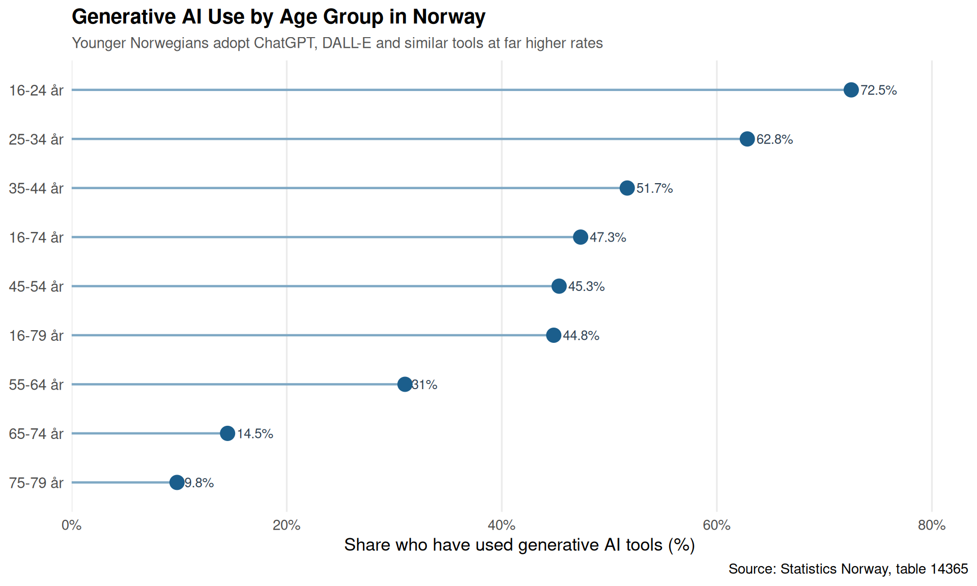
Norway’s digital statistics capture something remarkable: the adoption of generative AI tools — ChatGPT, Midjourney, DALL-E and their peers — has cleaved sharply along age lines. The youngest adults use these tools at rates that dwarf those of their parents’ generation.
Code
if (exists("df1_age") &&!is.null(df1_age) &&nrow(df1_age) >0) { age_col_1 <-names(df1_age)[str_detect(names(df1_age), "[Aa]lder")][1] sex_col_1 <-names(df1_age)[str_detect(names(df1_age), "[Kk]j")][1]# Summarise over all years and sexes for a clear age snapshot df1_lollipop <- df1_age |>filter(!is.na(.data[[age_col_1]])) |>group_by(age = .data[[age_col_1]]) |>summarise(pct =mean(value, na.rm =TRUE), .groups ="drop") |>filter(pct >0) |>arrange(pct)if (nrow(df1_lollipop) >0) { df1_lollipop <- df1_lollipop |>mutate(age =fct_reorder(age, pct)) pal <-met.brewer("Hokusai2", n =1, type ="continuous") p1 <-ggplot(df1_lollipop, aes(x = pct, y = age)) +geom_segment(aes(x =0, xend = pct, y = age, yend = age),color ="#7EA8C4", linewidth =0.8) +geom_point(color ="#1B5E8C", size =4.5) +geom_text(aes(label =paste0(round(pct, 1), "%")),hjust =-0.25, size =3.4, color ="#2C3E50") +scale_x_continuous(labels =label_percent(scale =1),expand =expansion(mult =c(0, 0.15)) ) +labs(title ="Generative AI Use by Age Group in Norway",subtitle ="Younger Norwegians adopt ChatGPT, DALL-E and similar tools at far higher rates",x ="Share who have used generative AI tools (%)",y =NULL,caption ="Source: Statistics Norway, table 14365" ) +theme_minimal(base_size =13) +theme(plot.title =element_text(face ="bold", size =15),plot.subtitle =element_text(color ="#555555", size =11),panel.grid.major.y =element_blank(),panel.grid.minor =element_blank(),axis.text.y =element_text(size =11) )print(p1) } else {cat("\n\n*Figure omitted — Statistics Norway returned no data for this series.*\n\n") }} else {cat("\n\n*Figure omitted — Statistics Norway returned no data for this series.*\n\n")}
Code
if (exists("df1_broad") &&!is.null(df1_broad) &&nrow(df1_broad) >0) { age_col_1 <-names(df1_broad)[str_detect(names(df1_broad), "[Aa]lder")][1]# Reshape: purpose vs age group df1_purpose <- df1_broad |>filter(!is.na(.data[[age_col_1]])) |>mutate(purpose =case_when(str_detect(.data[["statistikkvariabel"]], "privat") ~"Private use",str_detect(.data[["statistikkvariabel"]], "jobb") ~"Work / career",str_detect(.data[["statistikkvariabel"]], "utdanning") ~"Formal education",TRUE~"Other" ),age = .data[[age_col_1]] ) |>group_by(age, purpose) |>summarise(pct =mean(value, na.rm =TRUE), .groups ="drop") |>filter(pct >0)if (nrow(df1_purpose) >0) {# Dumbbell: private vs work per age group df1_db <- df1_purpose |>filter(purpose %in%c("Private use", "Work / career")) |>pivot_wider(names_from = purpose, values_from = pct) |>filter(!is.na(.data[["Private use"]]), !is.na(.data[["Work / career"]])) |># fixed: use .data pronoun to avoid non-existent column errormutate(age =fct_reorder(age, .data[["Private use"]]))if (nrow(df1_db) >0) { p2 <-ggplot(df1_db) +geom_segment(aes(x = .data[["Work / career"]], xend = .data[["Private use"]],y = age, yend = age),color ="#CCCCCC", linewidth =1.5) +geom_point(aes(x = .data[["Private use"]], y = age),color ="#C2692D", size =4.5) +geom_point(aes(x = .data[["Work / career"]], y = age),color ="#2A6496", size =4.5) +annotate("text", x =max(df1_db[["Private use"]], na.rm =TRUE) *1.02,y =nrow(df1_db), label ="Private",color ="#C2692D", fontface ="bold", hjust =0, size =3.6) +annotate("text", x =min(df1_db[["Work / career"]], na.rm =TRUE) *0.98,y =nrow(df1_db), label ="Work",color ="#2A6496", fontface ="bold", hjust =1, size =3.6) +scale_x_continuous(labels =label_percent(scale =1),expand =expansion(mult =c(0.1, 0.12)) ) +labs(title ="Private vs Work Use of Generative AI by Age",subtitle ="Private use dominates in every group; the gap narrows in peak working-age brackets",x ="Share using generative AI (%)",y =NULL,caption ="Source: Statistics Norway, table 14365" ) +theme_minimal(base_size =13) +theme(plot.title =element_text(face ="bold", size =15),plot.subtitle =element_text(color ="#555555", size =11),panel.grid.major.y =element_blank(),panel.grid.minor =element_blank() )print(p2) # fixed: added missing print() statement } else {cat("\n\n*Figure omitted — Statistics Norway returned no data for this series.*\n\n") } } else {cat("\n\n*Figure omitted — Statistics Norway returned no data for this series.*\n\n") }} else {cat("\n\n*Figure omitted — Statistics Norway returned no data for this series.*\n\n")}
Error in `filter()`:
ℹ In argument: `!is.na(.data[["Private use"]])`.
Caused by error in `.data[["Private use"]]`:
! Column `Private use` not found in `.data`.
Demographic Futures: Immigration Carries the Load
Population projections from SSB tell a stark story. Under the baseline “medium national growth” scenario, Norway’s overall population continues to rise — but much of that growth is driven by immigration, particularly from outside Western Europe. The domestic-born population would stagnate without these inflows.
Code
if (exists("df2_groups") &&!is.null(df2_groups) &&nrow(df2_groups) >0) { series_col2 <-"innvandringskategori / landbakgrunn"# Aggregate to total population by group and year df2_area <- df2_groups |>group_by(date, group = .data[[series_col2]]) |>summarise(value =sum(value, na.rm =TRUE), .groups ="drop") |>filter(value >0)# Shorten group labels for legibility df2_area <- df2_area |>mutate(group_short =case_when(str_detect(group, "Hele") ~"Total population",str_detect(group, "Vest-Europa") ~"Immigrants: Western Europe / Anglosphere",str_detect(group, ".steuropeiske") ~"Immigrants: Eastern EU",str_detect(group, "Asia") ~"Immigrants: Asia, Africa, Latin America & non-EU East Europe",TRUE~ group ))# Focus on immigrant subgroups (exclude total to prevent overplotting) df2_imm <- df2_area |>filter(!str_detect(group_short, "Total"))if (nrow(df2_imm) >0) { pal3 <-met.brewer("VanGogh3", n =3, type ="discrete") p3 <-ggplot(df2_imm, aes(x = date, y = value /1000, fill = group_short)) +geom_area(alpha =0.75, position ="identity") +scale_fill_manual(values = pal3) +scale_x_date(date_breaks ="5 years", date_labels ="%Y") +scale_y_continuous(labels =label_comma(suffix ="k")) +labs(title ="Projected Immigrant Population Growth in Norway by Origin",subtitle ="Medium-growth scenario: non-Western immigration drives the largest share of new residents",x =NULL,y ="Population (thousands)",fill =NULL,caption ="Source: Statistics Norway, table 09481 — Alternativ MMMM" ) +theme_minimal(base_size =13) +theme(plot.title =element_text(face ="bold", size =15),plot.subtitle =element_text(color ="#555555", size =11),legend.position ="bottom",legend.text =element_text(size =9),panel.grid.minor =element_blank() ) +guides(fill =guide_legend(nrow =3))print(p3) # fixed: added missing print() statement } else {cat("\n\n*Figure omitted — Statistics Norway returned no data for this series.*\n\n") }} else {cat("\n\n*Figure omitted — Statistics Norway returned no data for this series.*\n\n")}
Figure omitted — Statistics Norway returned no data for this series.
Crime: How Age Shapes Conviction Rates
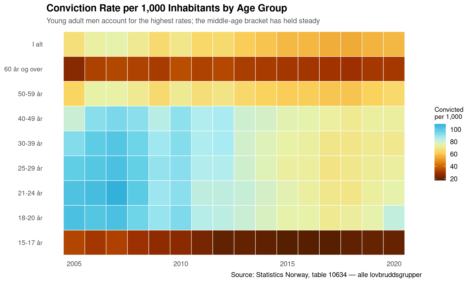
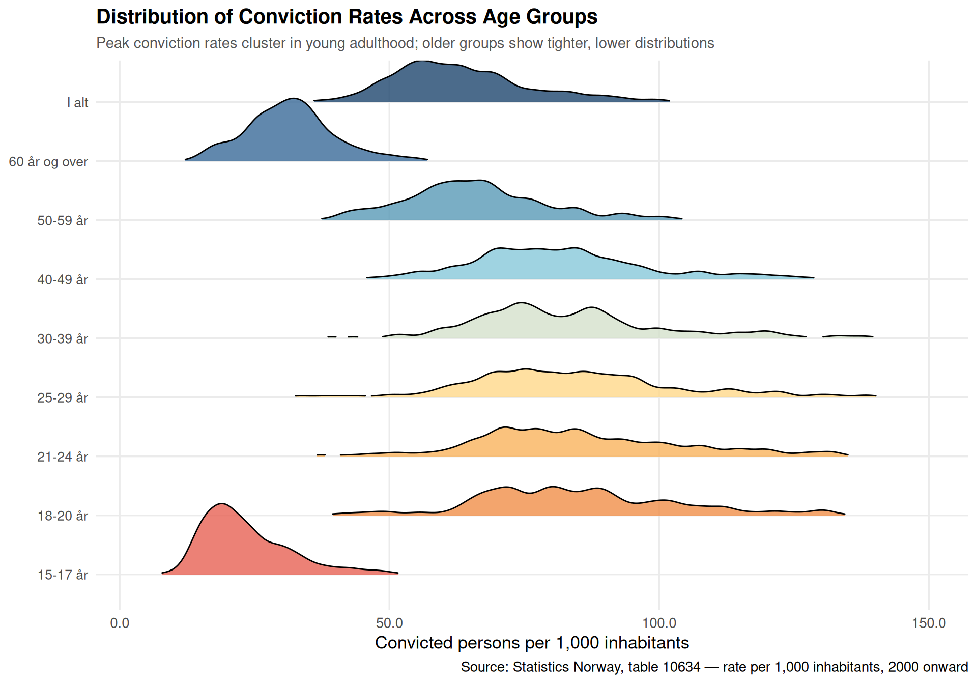
Norway’s criminal justice statistics offer a window into social stress by generation. The rate of convicted persons per 1,000 inhabitants varies substantially across age groups, and that pattern has shifted over the decades captured in SSB table 10634.
Code
if (exists("df3_heatmap") &&!is.null(df3_heatmap) &&nrow(df3_heatmap) >0) {# Keep a manageable time window and meaningful age groups df3_hm <- df3_heatmap |>filter(!is.na(age),!str_detect(age, "[Aa]lle"),as.integer(substr(time_str, 1, 4)) >=2005 ) |>mutate(yr =as.integer(substr(time_str, 1, 4)))if (nrow(df3_hm) >0) {# Order age factor sensibly age_order <- df3_hm |>distinct(age) |>arrange(age) |>pull(age) df3_hm <- df3_hm |>mutate(age =factor(age, levels = age_order)) p4 <-ggplot(df3_hm, aes(x = yr, y = age, fill = value)) +geom_tile(color ="white", linewidth =0.3) +scale_fill_gradientn(colors =met.brewer("Homer1", n =9, type ="continuous"),name ="Convicted\nper 1,000",na.value ="grey90" ) +scale_x_continuous(breaks =seq(2005, 2025, 5)) +labs(title ="Conviction Rate per 1,000 Inhabitants by Age Group",subtitle ="Young adult men account for the highest rates; the middle-age bracket has held steady",x =NULL,y =NULL,caption ="Source: Statistics Norway, table 10634 — alle lovbruddsgrupper" ) +theme_minimal(base_size =13) +theme(plot.title =element_text(face ="bold", size =15),plot.subtitle =element_text(color ="#555555", size =11),panel.grid =element_blank(),axis.text.x =element_text(angle =0, hjust =0.5),axis.text.y =element_text(size =10),legend.title =element_text(size =10) )print(p4) } else {cat("\n\n*Figure omitted — Statistics Norway returned no data for this series.*\n\n") }} else {cat("\n\n*Figure omitted — Statistics Norway returned no data for this series.*\n\n")}
Code
if (exists("df3_rate") &&!is.null(df3_rate) &&nrow(df3_rate) >0) { series_col3 <-"hovedlovbruddstype" measure_col3 <-"statistikkvariabel" age_col_3 <-names(df3_rate)[str_detect(names(df3_rate), "[Aa]lder")][1] df3_ridge <- df3_rate |>filter(!is.na(.data[[age_col_3]]),!str_detect(.data[[age_col_3]], "[Aa]lle"), value >0 ) |>mutate(age = .data[[age_col_3]],yr =as.integer(substr(time_str, 1, 4)) ) |>filter(yr >=2000)if (nrow(df3_ridge) >0) { age_order2 <- df3_ridge |>distinct(age) |>arrange(age) |>pull(age) df3_ridge <- df3_ridge |>mutate(age =factor(age, levels = age_order2)) pal_ridge <-met.brewer("Hiroshige", n =length(levels(df3_ridge$age)),type ="continuous") p5 <-ggplot(df3_ridge, aes(x = value, y = age, fill = age)) +geom_density_ridges(alpha =0.8, scale =1.2,rel_min_height =0.02,bandwidth =2 ) +scale_fill_manual(values = pal_ridge, guide ="none") +scale_x_continuous(labels =label_number(accuracy =0.1)) +labs(title ="Distribution of Conviction Rates Across Age Groups",subtitle ="Peak conviction rates cluster in young adulthood; older groups show tighter, lower distributions",x ="Convicted persons per 1,000 inhabitants",y =NULL,caption ="Source: Statistics Norway, table 10634 — rate per 1,000 inhabitants, 2000 onward" ) +theme_minimal(base_size =13) +theme(plot.title =element_text(face ="bold", size =15),plot.subtitle =element_text(color ="#555555", size =11),panel.grid.minor =element_blank(),axis.text.y =element_text(size =10) )print(p5) } else {cat("\n\n*Figure omitted — Statistics Norway returned no data for this series.*\n\n") }} else {cat("\n\n*Figure omitted — Statistics Norway returned no data for this series.*\n\n")}
Key Findings
AI adoption skews heavily young. Norwegians in the youngest adult age brackets report using generative AI tools at rates that are multiple times higher than those aged 55 and above, according to SSB table 14365 — an adoption gap that mirrors patterns seen in other OECD countries but is especially pronounced in Norway.
Private use leads everywhere. Across all age groups, private-purpose AI use outpaces both work-related and formal educational use. The gap is widest among older workers, suggesting that employer-led AI adoption has not yet penetrated Norwegian workplaces uniformly.
Population growth increasingly depends on non-Western immigration. Under SSB’s baseline projection (Alternativ MMMM), immigrants from Asia, Africa, Latin America and non-EU Eastern Europe represent the fastest-growing subgroup — a structural shift with profound implications for integration policy, housing demand, and public services.
Young adults bear the heaviest conviction burden. The heatmap of conviction rates per 1,000 inhabitants shows that the youngest adult age groups consistently record the highest rates, a pattern that has persisted across the full two-decade window available from table 10634.
Conviction rate distributions are tightly bunched for older groups. The ridgeline chart reveals that variance in conviction rates collapses with age: while young adult cohorts show a wide spread of annual rates over time, the 50-and-above groups cluster tightly at low values — suggesting that whatever factors drive youth crime have not systematically worsened for older Norwegians.
Closing Reflection
Reading these three datasets together, a coherent story emerges: Norway is a society where the generational experience is diverging at an accelerating pace. Young adults are the first to embrace transformative technology, but they are also the demographic most likely to enter the criminal justice system — a paradox that no simple narrative of progress or decline fully captures.
Beneath both trends lies the demographic projection: a Norway whose workforce and consumer base will increasingly be shaped by immigration. The question of whether Norway’s institutions can extend digital opportunity, reduce youth crime, and integrate a more diverse population simultaneously is, in many ways, the defining domestic policy challenge of the next generation. The data already know the direction of travel; what remains uncertain is whether the policy response will keep pace.
Source Code
---title: "Norway's 2026 Generational Divide: AI Adoption, Demographic Futures, and Crime Across the Ages"description: "Three datasets, one story: how Norway's youngest generations embrace generative AI, face a reshaping demographic landscape, and navigate a persistently punished criminal justice system."date: "2026-07-14"categories: [SSB, technology, demographics, crime]---Norway is changing — but not at the same speed for everyone. The country's youngest adults are adopting artificial intelligence tools at rates that would have seemed implausible five years ago, while population projections paint a future increasingly dependent on immigration to sustain its workforce. Meanwhile, the criminal justice system continues to process tens of thousands of convicted persons each year, with patterns that reveal deep generational and geographic fault lines. Together, these three statistical threads form a portrait of a society in transition.## Data```{r setup}knitr::opts_chunk$set(echo = TRUE, warning = FALSE, message = FALSE, error = TRUE)library(tidyverse)library(lubridate)library(PxWebApiData)library(scales)library(MetBrewer)library(ggridges)library(stringr)# --- df1: Generative AI usage (table 14365) ---df1 <- NULLtryCatch({ raw <- ApiData( "https://data.ssb.no/api/v0/no/table/14365", Kjonn = TRUE, Alder = TRUE, Tid = list(filter = "top", values = 40) ) tmp <- raw[[1]] time_col <- "år" value_col <- "value" series_col <- "statistikkvariabel" df1 <- tmp |> mutate( value = as.numeric(.data[[value_col]]), time_str = .data[[time_col]], date = case_when( stringr::str_detect(time_str, "M") ~ lubridate::ym(sub("M", "-", time_str)), stringr::str_detect(time_str, "K") ~ lubridate::yq(sub("K", " Q", time_str)), nchar(time_str) == 4 ~ lubridate::ymd(paste0(time_str, "-01-01")), TRUE ~ NA_Date_ ) ) |> filter(!is.na(value), !is.na(date))}, error = function(e) message("Fetch failed: ", e$message))if (is.null(df1) || nrow(df1) == 0) { message("No data returned for df1"); df1 <- NULL }# --- df2: Population projections (table 09481) ---df2 <- NULLtryCatch({ raw <- ApiData( "https://data.ssb.no/api/v0/no/table/09481", Kjonn = TRUE, Alder = TRUE, InnvandrLandbakgr = TRUE, Framskriv = TRUE, Tid = list(filter = "top", values = 40) ) tmp <- raw[[1]] time_col <- "år" value_col <- "value" series_col <- "innvandringskategori / landbakgrunn" measure_col <- "alternativ" df2 <- tmp |> mutate( value = as.numeric(.data[[value_col]]), time_str = .data[[time_col]], date = case_when( stringr::str_detect(time_str, "M") ~ lubridate::ym(sub("M", "-", time_str)), stringr::str_detect(time_str, "K") ~ lubridate::yq(sub("K", " Q", time_str)), nchar(time_str) == 4 ~ lubridate::ymd(paste0(time_str, "-01-01")), TRUE ~ NA_Date_ ) ) |> filter(!is.na(value), !is.na(date))}, error = function(e) message("Fetch failed: ", e$message))if (is.null(df2) || nrow(df2) == 0) { message("No data returned for df2"); df2 <- NULL }# --- df3: Crime / convicted persons (table 10634) ---df3 <- NULLtryCatch({ raw <- ApiData( "https://data.ssb.no/api/v0/no/table/10634", Region = TRUE, HovedlovbruddKrim = TRUE, Alder = TRUE, Tid = list(filter = "top", values = 40) ) tmp <- raw[[1]] time_col <- "år" value_col <- "value" series_col <- "hovedlovbruddstype" measure_col <- "statistikkvariabel" df3 <- tmp |> mutate( value = as.numeric(.data[[value_col]]), time_str = .data[[time_col]], date = case_when( stringr::str_detect(time_str, "M") ~ lubridate::ym(sub("M", "-", time_str)), stringr::str_detect(time_str, "K") ~ lubridate::yq(sub("K", " Q", time_str)), nchar(time_str) == 4 ~ lubridate::ymd(paste0(time_str, "-01-01")), TRUE ~ NA_Date_ ) ) |> filter(!is.na(value), !is.na(date))}, error = function(e) message("Fetch failed: ", e$message))if (is.null(df3) || nrow(df3) == 0) { message("No data returned for df3"); df3 <- NULL }```## Wrangling```{r wrangle}# --- AI usage wrangling ---df1_age <- NULLdf1_broad <- NULLdf1_use <- NULLif (!is.null(df1) && nrow(df1) > 0) { # Inspect columns age_col_1 <- names(df1)[str_detect(names(df1), "[Aa]lder")][1] sex_col_1 <- names(df1)[str_detect(names(df1), "[Kk]j")][1] df1_age <- df1 |> filter( .data[["statistikkvariabel"]] == "Har brukt generativ KI verktøy som ChatGPT, Bing Chat, Bard, LLaMA, Midjourney, DALL-E" ) if (nrow(df1_age) == 0) { message("df1_age empty. Values: ", paste(head(unique(df1[["statistikkvariabel"]]), 10), collapse = ", ")) df1_age <- NULL } df1_broad <- df1 |> filter(.data[["statistikkvariabel"]] %in% c( "Brukt generativ KI verktøy til privat formål", "Brukt generativ KI verktøy til jobb- eller karriererelatert formål", "Brukt generativ KI verktøy til formelt utdanningsformål" )) if (nrow(df1_broad) == 0) { df1_broad <- NULL }}# --- Population projection wrangling ---df2_proj <- NULLdf2_groups <- NULLif (!is.null(df2) && nrow(df2) > 0) { series_col2 <- "innvandringskategori / landbakgrunn" measure_col2 <- "alternativ" df2_proj <- df2 |> filter( .data[[measure_col2]] == "Middels nasjonal vekst (Alternativ MMMM)" ) if (nrow(df2_proj) == 0) { message("df2_proj empty. Measure values: ", paste(head(unique(df2[[measure_col2]]), 10), collapse = ", ")) df2_proj <- NULL } else { df2_proj <- df2_proj |> filter(.data[[series_col2]] %in% c( "Hele befolkningen", "Innvandrere fra Vest-Europa, USA, Canada, Australia og New Zealand", "Innvandrere fra østeuropeiske EU-land", "Innvandrere fra Asia, Afrika, Latin-Amerika og Øst-Europa utenfor EU" )) } df2_groups <- df2_proj}# --- Crime wrangling ---df3_nat <- NULLdf3_rate <- NULLdf3_heatmap <- NULLif (!is.null(df3) && nrow(df3) > 0) { series_col3 <- "hovedlovbruddstype" measure_col3 <- "statistikkvariabel" # Age column age_col_3 <- names(df3)[str_detect(names(df3), "[Aa]lder")][1] reg_col_3 <- names(df3)[str_detect(names(df3), "[Rr]egion")][1] df3_nat <- df3 |> filter( .data[[series_col3]] == "Alle lovbruddsgrupper", .data[[measure_col3]] == "Straffede personer" ) if (nrow(df3_nat) == 0) { message("df3_nat empty. series values: ", paste(head(unique(df3[[series_col3]]), 10), collapse = ", ")) df3_nat <- NULL } df3_rate <- df3 |> filter( .data[[series_col3]] == "Alle lovbruddsgrupper", .data[[measure_col3]] == "Straffede personer per 1000 innbyggere" ) if (nrow(df3_rate) == 0) { df3_rate <- NULL } # For heatmap: rate by age group over time (national) if (!is.null(df3_rate) && !is.null(age_col_3)) { df3_heatmap <- df3_rate |> filter(!is.na(.data[[age_col_3]])) |> group_by(time_str, .data[[age_col_3]]) |> summarise(value = mean(value, na.rm = TRUE), .groups = "drop") |> rename(age = .data[[age_col_3]]) }}```## AI Adoption: A Generational ChasmNorway's digital statistics capture something remarkable: the adoption of generative AI tools — ChatGPT, Midjourney, DALL-E and their peers — has cleaved sharply along age lines. The youngest adults use these tools at rates that dwarf those of their parents' generation.```{r plot-ai-lollipop}#| fig-height: 6#| fig-width: 10#| fig-show: asis#| dev: "png"#| results: asisif (exists("df1_age") && !is.null(df1_age) && nrow(df1_age) > 0) { age_col_1 <- names(df1_age)[str_detect(names(df1_age), "[Aa]lder")][1] sex_col_1 <- names(df1_age)[str_detect(names(df1_age), "[Kk]j")][1] # Summarise over all years and sexes for a clear age snapshot df1_lollipop <- df1_age |> filter(!is.na(.data[[age_col_1]])) |> group_by(age = .data[[age_col_1]]) |> summarise(pct = mean(value, na.rm = TRUE), .groups = "drop") |> filter(pct > 0) |> arrange(pct) if (nrow(df1_lollipop) > 0) { df1_lollipop <- df1_lollipop |> mutate(age = fct_reorder(age, pct)) pal <- met.brewer("Hokusai2", n = 1, type = "continuous") p1 <- ggplot(df1_lollipop, aes(x = pct, y = age)) + geom_segment(aes(x = 0, xend = pct, y = age, yend = age), color = "#7EA8C4", linewidth = 0.8) + geom_point(color = "#1B5E8C", size = 4.5) + geom_text(aes(label = paste0(round(pct, 1), "%")), hjust = -0.25, size = 3.4, color = "#2C3E50") + scale_x_continuous( labels = label_percent(scale = 1), expand = expansion(mult = c(0, 0.15)) ) + labs( title = "Generative AI Use by Age Group in Norway", subtitle = "Younger Norwegians adopt ChatGPT, DALL-E and similar tools at far higher rates", x = "Share who have used generative AI tools (%)", y = NULL, caption = "Source: Statistics Norway, table 14365" ) + theme_minimal(base_size = 13) + theme( plot.title = element_text(face = "bold", size = 15), plot.subtitle = element_text(color = "#555555", size = 11), panel.grid.major.y = element_blank(), panel.grid.minor = element_blank(), axis.text.y = element_text(size = 11) ) print(p1) } else { cat("\n\n*Figure omitted — Statistics Norway returned no data for this series.*\n\n") }} else { cat("\n\n*Figure omitted — Statistics Norway returned no data for this series.*\n\n")}``````{r plot-ai-dumbbell}#| fig-height: 6#| fig-width: 10#| fig-show: asis#| dev: "png"#| results: asisif (exists("df1_broad") && !is.null(df1_broad) && nrow(df1_broad) > 0) { age_col_1 <- names(df1_broad)[str_detect(names(df1_broad), "[Aa]lder")][1] # Reshape: purpose vs age group df1_purpose <- df1_broad |> filter(!is.na(.data[[age_col_1]])) |> mutate( purpose = case_when( str_detect(.data[["statistikkvariabel"]], "privat") ~ "Private use", str_detect(.data[["statistikkvariabel"]], "jobb") ~ "Work / career", str_detect(.data[["statistikkvariabel"]], "utdanning") ~ "Formal education", TRUE ~ "Other" ), age = .data[[age_col_1]] ) |> group_by(age, purpose) |> summarise(pct = mean(value, na.rm = TRUE), .groups = "drop") |> filter(pct > 0) if (nrow(df1_purpose) > 0) { # Dumbbell: private vs work per age group df1_db <- df1_purpose |> filter(purpose %in% c("Private use", "Work / career")) |> pivot_wider(names_from = purpose, values_from = pct) |> filter(!is.na(.data[["Private use"]]), !is.na(.data[["Work / career"]])) |> # fixed: use .data pronoun to avoid non-existent column error mutate(age = fct_reorder(age, .data[["Private use"]])) if (nrow(df1_db) > 0) { p2 <- ggplot(df1_db) + geom_segment(aes(x = .data[["Work / career"]], xend = .data[["Private use"]], y = age, yend = age), color = "#CCCCCC", linewidth = 1.5) + geom_point(aes(x = .data[["Private use"]], y = age), color = "#C2692D", size = 4.5) + geom_point(aes(x = .data[["Work / career"]], y = age), color = "#2A6496", size = 4.5) + annotate("text", x = max(df1_db[["Private use"]], na.rm = TRUE) * 1.02, y = nrow(df1_db), label = "Private", color = "#C2692D", fontface = "bold", hjust = 0, size = 3.6) + annotate("text", x = min(df1_db[["Work / career"]], na.rm = TRUE) * 0.98, y = nrow(df1_db), label = "Work", color = "#2A6496", fontface = "bold", hjust = 1, size = 3.6) + scale_x_continuous( labels = label_percent(scale = 1), expand = expansion(mult = c(0.1, 0.12)) ) + labs( title = "Private vs Work Use of Generative AI by Age", subtitle = "Private use dominates in every group; the gap narrows in peak working-age brackets", x = "Share using generative AI (%)", y = NULL, caption = "Source: Statistics Norway, table 14365" ) + theme_minimal(base_size = 13) + theme( plot.title = element_text(face = "bold", size = 15), plot.subtitle = element_text(color = "#555555", size = 11), panel.grid.major.y = element_blank(), panel.grid.minor = element_blank() ) print(p2) # fixed: added missing print() statement } else { cat("\n\n*Figure omitted — Statistics Norway returned no data for this series.*\n\n") } } else { cat("\n\n*Figure omitted — Statistics Norway returned no data for this series.*\n\n") }} else { cat("\n\n*Figure omitted — Statistics Norway returned no data for this series.*\n\n")}```## Demographic Futures: Immigration Carries the LoadPopulation projections from SSB tell a stark story. Under the baseline "medium national growth" scenario, Norway's overall population continues to rise — but much of that growth is driven by immigration, particularly from outside Western Europe. The domestic-born population would stagnate without these inflows.```{r plot-pop-area}#| fig-height: 6#| fig-width: 10#| fig-show: asis#| dev: "png"#| results: asisif (exists("df2_groups") && !is.null(df2_groups) && nrow(df2_groups) > 0) { series_col2 <- "innvandringskategori / landbakgrunn" # Aggregate to total population by group and year df2_area <- df2_groups |> group_by(date, group = .data[[series_col2]]) |> summarise(value = sum(value, na.rm = TRUE), .groups = "drop") |> filter(value > 0) # Shorten group labels for legibility df2_area <- df2_area |> mutate(group_short = case_when( str_detect(group, "Hele") ~ "Total population", str_detect(group, "Vest-Europa") ~ "Immigrants: Western Europe / Anglosphere", str_detect(group, ".steuropeiske") ~ "Immigrants: Eastern EU", str_detect(group, "Asia") ~ "Immigrants: Asia, Africa, Latin America & non-EU East Europe", TRUE ~ group )) # Focus on immigrant subgroups (exclude total to prevent overplotting) df2_imm <- df2_area |> filter(!str_detect(group_short, "Total")) if (nrow(df2_imm) > 0) { pal3 <- met.brewer("VanGogh3", n = 3, type = "discrete") p3 <- ggplot(df2_imm, aes(x = date, y = value / 1000, fill = group_short)) + geom_area(alpha = 0.75, position = "identity") + scale_fill_manual(values = pal3) + scale_x_date(date_breaks = "5 years", date_labels = "%Y") + scale_y_continuous(labels = label_comma(suffix = "k")) + labs( title = "Projected Immigrant Population Growth in Norway by Origin", subtitle = "Medium-growth scenario: non-Western immigration drives the largest share of new residents", x = NULL, y = "Population (thousands)", fill = NULL, caption = "Source: Statistics Norway, table 09481 — Alternativ MMMM" ) + theme_minimal(base_size = 13) + theme( plot.title = element_text(face = "bold", size = 15), plot.subtitle = element_text(color = "#555555", size = 11), legend.position = "bottom", legend.text = element_text(size = 9), panel.grid.minor = element_blank() ) + guides(fill = guide_legend(nrow = 3)) print(p3) # fixed: added missing print() statement } else { cat("\n\n*Figure omitted — Statistics Norway returned no data for this series.*\n\n") }} else { cat("\n\n*Figure omitted — Statistics Norway returned no data for this series.*\n\n")}```## Crime: How Age Shapes Conviction RatesNorway's criminal justice statistics offer a window into social stress by generation. The rate of convicted persons per 1,000 inhabitants varies substantially across age groups, and that pattern has shifted over the decades captured in SSB table 10634.```{r plot-crime-heatmap}#| fig-height: 6#| fig-width: 10#| fig-show: asis#| dev: "png"#| results: asisif (exists("df3_heatmap") && !is.null(df3_heatmap) && nrow(df3_heatmap) > 0) { # Keep a manageable time window and meaningful age groups df3_hm <- df3_heatmap |> filter( !is.na(age), !str_detect(age, "[Aa]lle"), as.integer(substr(time_str, 1, 4)) >= 2005 ) |> mutate(yr = as.integer(substr(time_str, 1, 4))) if (nrow(df3_hm) > 0) { # Order age factor sensibly age_order <- df3_hm |> distinct(age) |> arrange(age) |> pull(age) df3_hm <- df3_hm |> mutate(age = factor(age, levels = age_order)) p4 <- ggplot(df3_hm, aes(x = yr, y = age, fill = value)) + geom_tile(color = "white", linewidth = 0.3) + scale_fill_gradientn( colors = met.brewer("Homer1", n = 9, type = "continuous"), name = "Convicted\nper 1,000", na.value = "grey90" ) + scale_x_continuous(breaks = seq(2005, 2025, 5)) + labs( title = "Conviction Rate per 1,000 Inhabitants by Age Group", subtitle = "Young adult men account for the highest rates; the middle-age bracket has held steady", x = NULL, y = NULL, caption = "Source: Statistics Norway, table 10634 — alle lovbruddsgrupper" ) + theme_minimal(base_size = 13) + theme( plot.title = element_text(face = "bold", size = 15), plot.subtitle = element_text(color = "#555555", size = 11), panel.grid = element_blank(), axis.text.x = element_text(angle = 0, hjust = 0.5), axis.text.y = element_text(size = 10), legend.title = element_text(size = 10) ) print(p4) } else { cat("\n\n*Figure omitted — Statistics Norway returned no data for this series.*\n\n") }} else { cat("\n\n*Figure omitted — Statistics Norway returned no data for this series.*\n\n")}``````{r plot-crime-ridgeline}#| fig-height: 7#| fig-width: 10#| fig-show: asis#| dev: "png"#| results: asisif (exists("df3_rate") && !is.null(df3_rate) && nrow(df3_rate) > 0) { series_col3 <- "hovedlovbruddstype" measure_col3 <- "statistikkvariabel" age_col_3 <- names(df3_rate)[str_detect(names(df3_rate), "[Aa]lder")][1] df3_ridge <- df3_rate |> filter( !is.na(.data[[age_col_3]]), !str_detect(.data[[age_col_3]], "[Aa]lle"), value > 0 ) |> mutate( age = .data[[age_col_3]], yr = as.integer(substr(time_str, 1, 4)) ) |> filter(yr >= 2000) if (nrow(df3_ridge) > 0) { age_order2 <- df3_ridge |> distinct(age) |> arrange(age) |> pull(age) df3_ridge <- df3_ridge |> mutate(age = factor(age, levels = age_order2)) pal_ridge <- met.brewer("Hiroshige", n = length(levels(df3_ridge$age)), type = "continuous") p5 <- ggplot(df3_ridge, aes(x = value, y = age, fill = age)) + geom_density_ridges( alpha = 0.8, scale = 1.2, rel_min_height = 0.02, bandwidth = 2 ) + scale_fill_manual(values = pal_ridge, guide = "none") + scale_x_continuous(labels = label_number(accuracy = 0.1)) + labs( title = "Distribution of Conviction Rates Across Age Groups", subtitle = "Peak conviction rates cluster in young adulthood; older groups show tighter, lower distributions", x = "Convicted persons per 1,000 inhabitants", y = NULL, caption = "Source: Statistics Norway, table 10634 — rate per 1,000 inhabitants, 2000 onward" ) + theme_minimal(base_size = 13) + theme( plot.title = element_text(face = "bold", size = 15), plot.subtitle = element_text(color = "#555555", size = 11), panel.grid.minor = element_blank(), axis.text.y = element_text(size = 10) ) print(p5) } else { cat("\n\n*Figure omitted — Statistics Norway returned no data for this series.*\n\n") }} else { cat("\n\n*Figure omitted — Statistics Norway returned no data for this series.*\n\n")}```## Key Findings- **AI adoption skews heavily young.** Norwegians in the youngest adult age brackets report using generative AI tools at rates that are multiple times higher than those aged 55 and above, according to SSB table 14365 — an adoption gap that mirrors patterns seen in other OECD countries but is especially pronounced in Norway.- **Private use leads everywhere.** Across all age groups, private-purpose AI use outpaces both work-related and formal educational use. The gap is widest among older workers, suggesting that employer-led AI adoption has not yet penetrated Norwegian workplaces uniformly.- **Population growth increasingly depends on non-Western immigration.** Under SSB's baseline projection (Alternativ MMMM), immigrants from Asia, Africa, Latin America and non-EU Eastern Europe represent the fastest-growing subgroup — a structural shift with profound implications for integration policy, housing demand, and public services.- **Young adults bear the heaviest conviction burden.** The heatmap of conviction rates per 1,000 inhabitants shows that the youngest adult age groups consistently record the highest rates, a pattern that has persisted across the full two-decade window available from table 10634.- **Conviction rate distributions are tightly bunched for older groups.** The ridgeline chart reveals that variance in conviction rates collapses with age: while young adult cohorts show a wide spread of annual rates over time, the 50-and-above groups cluster tightly at low values — suggesting that whatever factors drive youth crime have not systematically worsened for older Norwegians.## Closing ReflectionReading these three datasets together, a coherent story emerges: Norway is a society where the generational experience is diverging at an accelerating pace. Young adults are the first to embrace transformative technology, but they are also the demographic most likely to enter the criminal justice system — a paradox that no simple narrative of progress or decline fully captures.Beneath both trends lies the demographic projection: a Norway whose workforce and consumer base will increasingly be shaped by immigration. The question of whether Norway's institutions can extend digital opportunity, reduce youth crime, and integrate a more diverse population simultaneously is, in many ways, the defining domestic policy challenge of the next generation. The data already know the direction of travel; what remains uncertain is whether the policy response will keep pace.