New SSB data reveal stark age and gender gaps in generative AI adoption among Norwegians, while housing completions track a separate but converging crisis in the physical economy.
Published
July 13, 2026
Norway is simultaneously navigating two structural transitions that will define its economic trajectory for the next decade: the rapid diffusion of generative artificial intelligence into everyday work and study, and a deepening contraction in residential construction. The first shapes who gets ahead in the labour market; the second shapes where and how Norwegians can afford to live. Together they point toward a society fracturing along lines of age, skill, and geography.
Data
Statistics Norway’s table 14365 tracks the share of Norwegians who have used generative AI tools — ChatGPT, Bing Chat, Bard, DALL-E, and similar — broken down by sex and age group. Table 06512 records housing construction permits and completions, distinguishing between all dwellings and apartments specifically, giving a granular view of supply-side dynamics in the housing market.
# --- df1: generative AI adoption ---df1_overall <-NULLdf1_gender <-NULLdf1_age <-NULLdf1_purpose <-NULLif (!is.null(df1) &&nrow(df1) >0) {# Inspect available columns ai_series_col <-"statistikkvariabel"# All unique series values series_vals <-unique(df1[[ai_series_col]])# Build a lookup for the four AI use-purpose series purpose_labels <-c("Har brukt generativ KI verktøy som ChatGPT, Bing Chat, Bard, LLaMA, Midjourney, DALL-E","Brukt generativ KI verktøy til privat formål","Brukt generativ KI verktøy til jobb- eller karriererelatert formål","Brukt generativ KI verktøy til formelt utdanningsformål, f.eks. skole eller universitet" )# Filter to rows that match any of these series df1_purpose <- df1 |>filter(.data[[ai_series_col]] %in% purpose_labels)if (nrow(df1_purpose) ==0) {message("df1_purpose empty. Series vals: ", paste(head(series_vals, 10), collapse ="; ")) df1_purpose <-NULL }# Overall adoption (first series) df1_overall <- df1 |>filter(.data[[ai_series_col]] == purpose_labels[1])if (nrow(df1_overall) ==0) { df1_overall <-NULL }# Gender breakdown — check for Kjønn columnif ("kjønn"%in%names(df1)) { df1_gender <- df1 |>filter( .data[[ai_series_col]] == purpose_labels[1],!is.na(kjønn), kjønn !="Begge kjønn", kjønn !="0" )if (nrow(df1_gender) ==0) df1_gender <-NULL }# Age breakdownif ("alder"%in%names(df1)) { df1_age <- df1 |>filter( .data[[ai_series_col]] == purpose_labels[1],!is.na(alder), alder !="16-79 år", alder !="Alle" )if (nrow(df1_age) ==0) df1_age <-NULL }}# --- df2: housing construction ---df2_long <-NULLdf2_permits <-NULLdf2_completed <-NULLdf2_dumbbell <-NULLif (!is.null(df2) &&nrow(df2) >0) { housing_series_col <-"statistikkvariabel" housing_vals <-unique(df2[[housing_series_col]]) df2_long <- df2 |>filter(.data[[housing_series_col]] %in%c("Igangsettingstillatelser boliger","Igangsettingstillatelser leiligheter","Fullførte boliger","Fullførte leiligheter" )) |>mutate(yr = lubridate::year(date),series = .data[[housing_series_col]] )if (nrow(df2_long) ==0) {message("df2_long empty. Values: ", paste(head(housing_vals, 10), collapse ="; ")) df2_long <-NULL } else { df2_permits <- df2_long |>filter(series %in%c("Igangsettingstillatelser boliger","Igangsettingstillatelser leiligheter")) df2_completed <- df2_long |>filter(series %in%c("Fullførte boliger","Fullførte leiligheter"))# Dumbbell: permits vs completions for all dwellings df2_dumbbell <- df2_long |>filter(series %in%c("Igangsettingstillatelser boliger","Fullførte boliger")) |>select(yr, series, value) |>pivot_wider(names_from = series, values_from = value) |>rename(permits =`Igangsettingstillatelser boliger`,completed =`Fullførte boliger` ) |>filter(!is.na(permits), !is.na(completed))if (nrow(df2_dumbbell) ==0) df2_dumbbell <-NULL }}
Norway’s Generative AI Adoption: A Snapshot of the Digital Divide
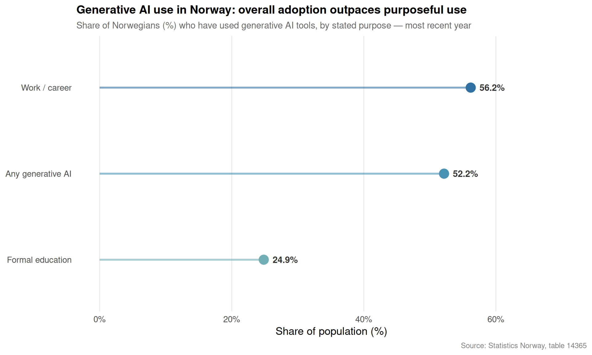
The share of Norwegians who have used a generative AI tool — ChatGPT being the most prominent example — has grown rapidly since these tools became widely available. But that aggregate figure conceals large differences by age and stated purpose, with implications for how the labour market will evolve.
Code
if (exists("df1_purpose") &&!is.null(df1_purpose) &&nrow(df1_purpose) >0) {# Summarise by series — take the most recent year's average or latest value df1_purpose_sum <- df1_purpose |>group_by(.data[["statistikkvariabel"]]) |>filter(date ==max(date)) |>summarise(mean_val =mean(value, na.rm =TRUE), .groups ="drop") |>arrange(mean_val) |>mutate(label_short =case_when( stringr::str_detect(statistikkvariabel, "privat") ~"Private use", stringr::str_detect(statistikkvariabel, "jobb") ~"Work / career", stringr::str_detect(statistikkvariabel, "utdanning") ~"Formal education", stringr::str_detect(statistikkvariabel, "Har brukt") ~"Any generative AI",TRUE~ statistikkvariabel ),label_short =factor(label_short, levels = label_short) ) pal <-met.brewer("Hokusai2", n =4) p1 <-ggplot(df1_purpose_sum,aes(x = mean_val, y = label_short, colour = label_short)) +geom_segment(aes(x =0, xend = mean_val, yend = label_short),linewidth =1.1, alpha =0.6) +geom_point(size =5) +geom_text(aes(label =paste0(round(mean_val, 1), "%")),hjust =-0.35, size =3.8, fontface ="bold", colour ="grey20") +scale_x_continuous(limits =c(0, max(df1_purpose_sum$mean_val, na.rm =TRUE) *1.25),labels =label_number(suffix ="%") ) +scale_colour_manual(values = pal) +labs(title ="Generative AI use in Norway: overall adoption outpaces purposeful use",subtitle ="Share of Norwegians (%) who have used generative AI tools, by stated purpose — most recent year",x ="Share of population (%)",y =NULL,caption ="Source: Statistics Norway, table 14365" ) +theme_minimal(base_size =13) +theme(legend.position ="none",panel.grid.major.y =element_blank(),panel.grid.minor =element_blank(),plot.title =element_text(face ="bold", size =14),plot.subtitle =element_text(colour ="grey40", size =11),plot.caption =element_text(colour ="grey50", size =9) )print(p1)} else {cat("\n\n*Figure omitted — Statistics Norway returned no data for this series.*\n\n")}
Code
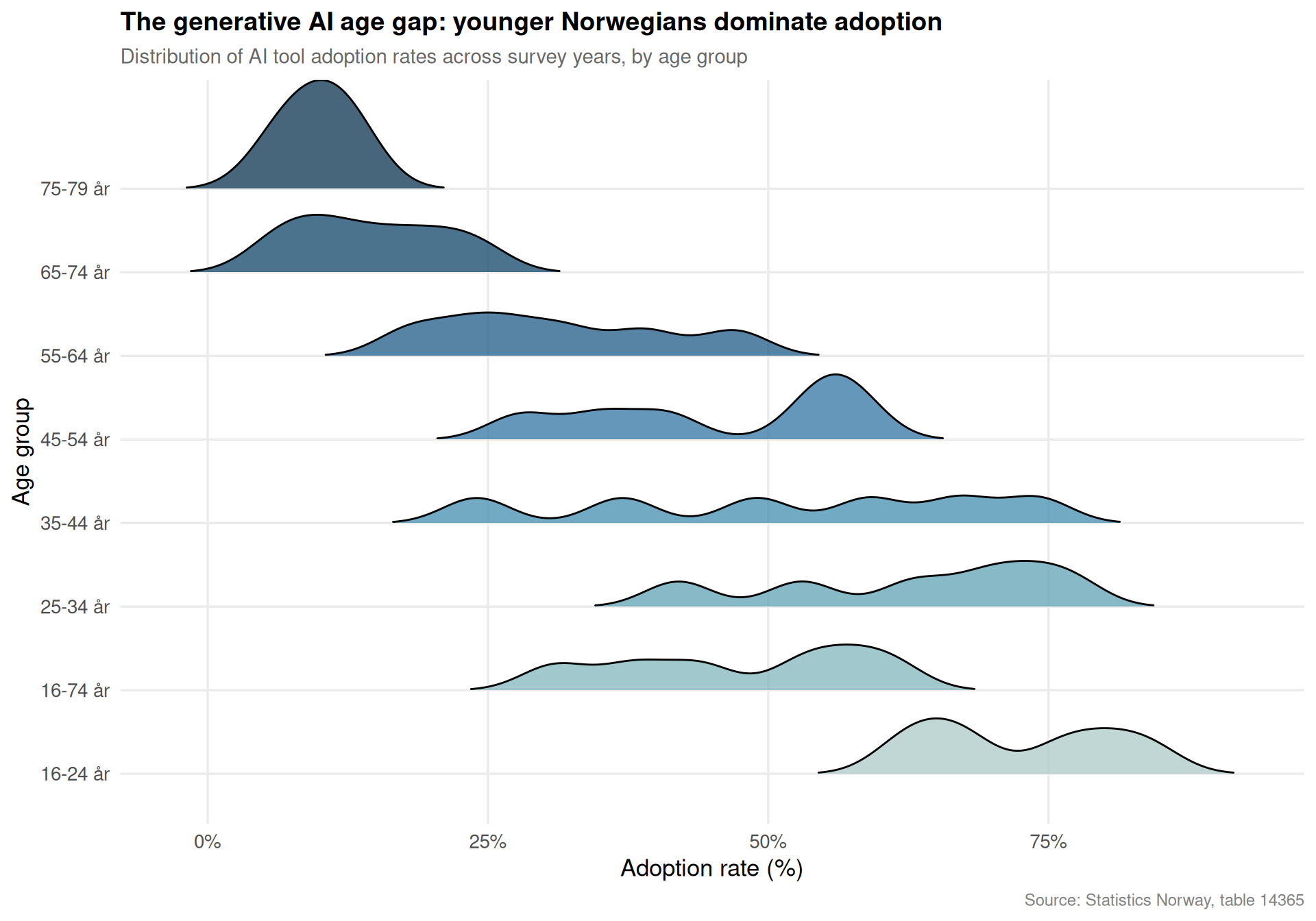
if (exists("df1_age") &&!is.null(df1_age) &&nrow(df1_age) >0) { pal2 <-met.brewer("Hokusai2", n =length(unique(df1_age$alder))) p2 <-ggplot(df1_age,aes(x = value, y = alder, fill = alder)) + ggridges::geom_density_ridges(scale =1.3, alpha =0.75, bandwidth =3,rel_min_height =0.01 ) +scale_x_continuous(labels =label_number(suffix ="%")) +scale_fill_manual(values = pal2) +labs(title ="The generative AI age gap: younger Norwegians dominate adoption",subtitle ="Distribution of AI tool adoption rates across survey years, by age group",x ="Adoption rate (%)",y ="Age group",caption ="Source: Statistics Norway, table 14365" ) +theme_minimal(base_size =13) +theme(legend.position ="none",panel.grid.minor =element_blank(),plot.title =element_text(face ="bold", size =14),plot.subtitle =element_text(colour ="grey40", size =11),plot.caption =element_text(colour ="grey50", size =9) )print(p2)} else {cat("\n\n*Figure omitted — Statistics Norway returned no data for this series.*\n\n")}
The ridgeline chart above captures something crucial: generative AI is not a monolithic phenomenon sweeping all of Norway at once. It is concentrated among the young. Older workers, precisely those already navigating a labour market that values adaptability, are the least likely to have engaged with these tools. Whether that gap reflects preference, access, or a mismatch in training opportunities, the effect on long-term employability is the same.
Error in `max()`:
! invalid 'type' (list) of argument
Housing Construction: Supply Failure in the Physical Economy
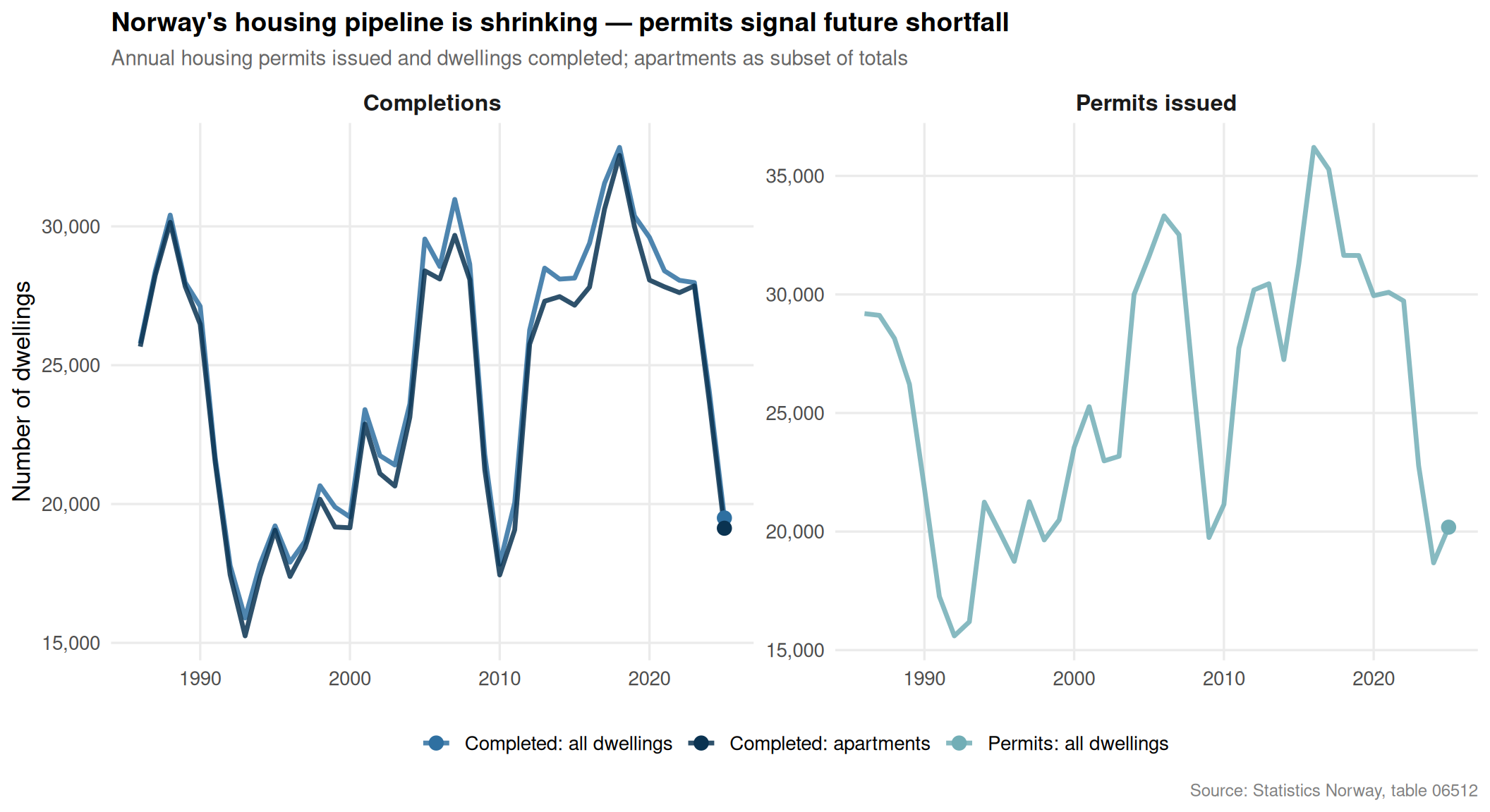
While the digital economy races ahead for some, the physical economy tells a different story. Residential construction — the key mechanism through which housing supply responds to demand — has been slowing. Fewer permits mean fewer completions several years down the line, locking in undersupply precisely when demographic pressure is greatest in city regions.
Code
if (exists("df2_long") &&!is.null(df2_long) &&nrow(df2_long) >0) {# Clean labels for display df2_plot <- df2_long |>mutate(series_label =case_when( series =="Igangsettingstillatelser boliger"~"Permits: all dwellings", series =="Igangsettingstillatelser leiligheter"~"Permits: apartments", series =="Fullførte boliger"~"Completed: all dwellings", series =="Fullførte leiligheter"~"Completed: apartments",TRUE~ series ),category =if_else( stringr::str_detect(series, "Igangsett"),"Permits issued", "Completions" ) ) pal4 <-met.brewer("Hokusai2", n =4)names(pal4) <-c("Permits: all dwellings", "Permits: apartments","Completed: all dwellings", "Completed: apartments") p4 <-ggplot(df2_plot,aes(x = date, y = value, colour = series_label, group = series_label)) +geom_line(linewidth =1.2, alpha =0.85) +geom_point(data = df2_plot |>group_by(series_label) |>filter(date ==max(date)),size =3) +facet_wrap(~ category, ncol =2, scales ="free_y") +scale_y_continuous(labels =label_comma()) +scale_colour_manual(values = pal4) +labs(title ="Norway's housing pipeline is shrinking — permits signal future shortfall",subtitle ="Annual housing permits issued and dwellings completed; apartments as subset of totals",x =NULL,y ="Number of dwellings",colour =NULL,caption ="Source: Statistics Norway, table 06512" ) +theme_minimal(base_size =13) +theme(legend.position ="bottom",panel.grid.minor =element_blank(),strip.text =element_text(face ="bold", size =12),plot.title =element_text(face ="bold", size =14),plot.subtitle =element_text(colour ="grey40", size =11),plot.caption =element_text(colour ="grey50", size =9) )print(p4)} else {cat("\n\n*Figure omitted — Statistics Norway returned no data for this series.*\n\n")}
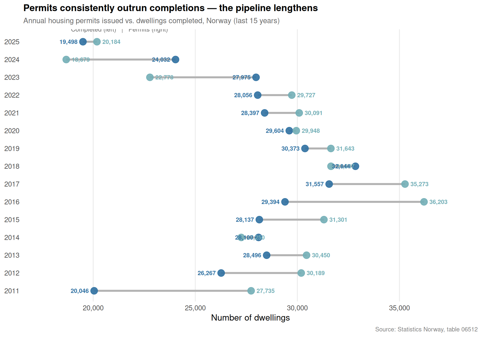
The dumbbell chart makes a structural pattern visible: in most years, the number of permits issued exceeds the number of dwellings actually completed. That gap represents projects delayed, cancelled, or stretched across multiple budget cycles. When construction costs rise sharply — as they have in Norway since 2021 — the conversion rate from permit to key deteriorates further, compressing the effective housing supply even when headline permit numbers look reasonable.
Key Findings
Generative AI adoption is real but uneven. The share of Norwegians who have used a tool such as ChatGPT or DALL-E has climbed meaningfully, but use for formal work and education purposes lags well behind overall experimentation, suggesting shallow rather than transformative adoption.
Age is the dominant fault line. Younger Norwegians are substantially more likely to have used generative AI than those over 50. Given that older workers are already more exposed to labour market disruption, the gap risks compounding existing inequalities rather than flattening them.
A gender gap persists. Men report higher generative AI adoption than women across available survey years, a pattern that mirrors global findings and raises questions about whether AI-related productivity gains will accrue equitably across Norway’s otherwise relatively equal workforce.
Housing permits have trended downward from recent peaks. The number of new permits issued for both total dwellings and apartments specifically has declined from highs seen in the mid-2010s, a warning signal for housing supply in the years ahead.
The permit-to-completion gap is structural. In nearly every recent year, fewer dwellings were completed than permits would imply, pointing to a pipeline that is both shrinking in volume and becoming less efficient at converting intentions into actual homes.
Closing Reflection
Norway faces a version of a challenge familiar to most advanced economies, but shaped by its specific geography of oil wealth, flat wage structures, and strong welfare institutions. The generative AI transition rewards those already equipped with digital literacy and professional networks; the housing squeeze punishes those who most need affordable urban accommodation — frequently the same younger, lower-income cohorts now being told their careers depend on mastering tools many employers have barely begun to evaluate. Neither trend is yet a crisis, but the direction of travel is clear. Closing the digital adoption gap and rebuilding the housing pipeline are not separate policy questions: they are two sides of the same structural wager on whether Norway’s prosperity will remain broadly shared.
Source Code
---title: "Norway's 2026 Digital Divide: Who Adopts Generative AI and How Housing Construction Signals Economic Fracture"description: "New SSB data reveal stark age and gender gaps in generative AI adoption among Norwegians, while housing completions track a separate but converging crisis in the physical economy."date: "2026-07-13"categories: [SSB, technology, housing, labour-market, digital-economy]---Norway is simultaneously navigating two structural transitions that will define its economic trajectory for the next decade: the rapid diffusion of generative artificial intelligence into everyday work and study, and a deepening contraction in residential construction. The first shapes who gets ahead in the labour market; the second shapes where and how Norwegians can afford to live. Together they point toward a society fracturing along lines of age, skill, and geography.## DataStatistics Norway's table 14365 tracks the share of Norwegians who have used generative AI tools — ChatGPT, Bing Chat, Bard, DALL-E, and similar — broken down by sex and age group. Table 06512 records housing construction permits and completions, distinguishing between all dwellings and apartments specifically, giving a granular view of supply-side dynamics in the housing market.```{r setup}knitr::opts_chunk$set(echo = TRUE, warning = FALSE, message = FALSE, error = TRUE)library(tidyverse)library(lubridate)library(PxWebApiData)library(scales)library(MetBrewer)library(ggridges)df1 <- NULLtryCatch({ raw <- ApiData( "https://data.ssb.no/api/v0/no/table/14365", Kjonn = TRUE, Alder = TRUE, Tid = list(filter = "top", values = 40) ) tmp <- raw[[1]] time_col <- "år" value_col <- "value" series_col <- "statistikkvariabel" df1 <- tmp |> mutate( value = as.numeric(.data[[value_col]]), time_str = .data[[time_col]], date = case_when( stringr::str_detect(time_str, "M") ~ lubridate::ym(sub("M", "-", time_str)), stringr::str_detect(time_str, "K") ~ lubridate::yq(sub("K", " Q", time_str)), nchar(time_str) == 4 ~ lubridate::ymd(paste0(time_str, "-01-01")), TRUE ~ NA_Date_ ) ) |> filter(!is.na(value), !is.na(date))}, error = function(e) message("Fetch failed: ", e$message))if (is.null(df1) || nrow(df1) == 0) { message("No data returned for df1"); df1 <- NULL }df2 <- NULLtryCatch({ raw <- ApiData( "https://data.ssb.no/api/v0/no/table/06512", Tid = list(filter = "top", values = 40) ) tmp <- raw[[1]] time_col <- "år" value_col <- "value" series_col <- "statistikkvariabel" df2 <- tmp |> mutate( value = as.numeric(.data[[value_col]]), time_str = .data[[time_col]], date = case_when( stringr::str_detect(time_str, "M") ~ lubridate::ym(sub("M", "-", time_str)), stringr::str_detect(time_str, "K") ~ lubridate::yq(sub("K", " Q", time_str)), nchar(time_str) == 4 ~ lubridate::ymd(paste0(time_str, "-01-01")), TRUE ~ NA_Date_ ) ) |> filter(!is.na(value), !is.na(date))}, error = function(e) message("Fetch failed: ", e$message))if (is.null(df2) || nrow(df2) == 0) { message("No data returned for df2"); df2 <- NULL }```## Wrangling```{r wrangle}# --- df1: generative AI adoption ---df1_overall <- NULLdf1_gender <- NULLdf1_age <- NULLdf1_purpose <- NULLif (!is.null(df1) && nrow(df1) > 0) { # Inspect available columns ai_series_col <- "statistikkvariabel" # All unique series values series_vals <- unique(df1[[ai_series_col]]) # Build a lookup for the four AI use-purpose series purpose_labels <- c( "Har brukt generativ KI verktøy som ChatGPT, Bing Chat, Bard, LLaMA, Midjourney, DALL-E", "Brukt generativ KI verktøy til privat formål", "Brukt generativ KI verktøy til jobb- eller karriererelatert formål", "Brukt generativ KI verktøy til formelt utdanningsformål, f.eks. skole eller universitet" ) # Filter to rows that match any of these series df1_purpose <- df1 |> filter(.data[[ai_series_col]] %in% purpose_labels) if (nrow(df1_purpose) == 0) { message("df1_purpose empty. Series vals: ", paste(head(series_vals, 10), collapse = "; ")) df1_purpose <- NULL } # Overall adoption (first series) df1_overall <- df1 |> filter(.data[[ai_series_col]] == purpose_labels[1]) if (nrow(df1_overall) == 0) { df1_overall <- NULL } # Gender breakdown — check for Kjønn column if ("kjønn" %in% names(df1)) { df1_gender <- df1 |> filter( .data[[ai_series_col]] == purpose_labels[1], !is.na(kjønn), kjønn != "Begge kjønn", kjønn != "0" ) if (nrow(df1_gender) == 0) df1_gender <- NULL } # Age breakdown if ("alder" %in% names(df1)) { df1_age <- df1 |> filter( .data[[ai_series_col]] == purpose_labels[1], !is.na(alder), alder != "16-79 år", alder != "Alle" ) if (nrow(df1_age) == 0) df1_age <- NULL }}# --- df2: housing construction ---df2_long <- NULLdf2_permits <- NULLdf2_completed <- NULLdf2_dumbbell <- NULLif (!is.null(df2) && nrow(df2) > 0) { housing_series_col <- "statistikkvariabel" housing_vals <- unique(df2[[housing_series_col]]) df2_long <- df2 |> filter(.data[[housing_series_col]] %in% c( "Igangsettingstillatelser boliger", "Igangsettingstillatelser leiligheter", "Fullførte boliger", "Fullførte leiligheter" )) |> mutate( yr = lubridate::year(date), series = .data[[housing_series_col]] ) if (nrow(df2_long) == 0) { message("df2_long empty. Values: ", paste(head(housing_vals, 10), collapse = "; ")) df2_long <- NULL } else { df2_permits <- df2_long |> filter(series %in% c("Igangsettingstillatelser boliger", "Igangsettingstillatelser leiligheter")) df2_completed <- df2_long |> filter(series %in% c("Fullførte boliger", "Fullførte leiligheter")) # Dumbbell: permits vs completions for all dwellings df2_dumbbell <- df2_long |> filter(series %in% c("Igangsettingstillatelser boliger", "Fullførte boliger")) |> select(yr, series, value) |> pivot_wider(names_from = series, values_from = value) |> rename( permits = `Igangsettingstillatelser boliger`, completed = `Fullførte boliger` ) |> filter(!is.na(permits), !is.na(completed)) if (nrow(df2_dumbbell) == 0) df2_dumbbell <- NULL }}```## Norway's Generative AI Adoption: A Snapshot of the Digital DivideThe share of Norwegians who have used a generative AI tool — ChatGPT being the most prominent example — has grown rapidly since these tools became widely available. But that aggregate figure conceals large differences by age and stated purpose, with implications for how the labour market will evolve.```{r plot-ai-lollipop}#| fig-height: 6#| fig-width: 10#| fig-show: asis#| dev: "png"#| results: asisif (exists("df1_purpose") && !is.null(df1_purpose) && nrow(df1_purpose) > 0) { # Summarise by series — take the most recent year's average or latest value df1_purpose_sum <- df1_purpose |> group_by(.data[["statistikkvariabel"]]) |> filter(date == max(date)) |> summarise(mean_val = mean(value, na.rm = TRUE), .groups = "drop") |> arrange(mean_val) |> mutate( label_short = case_when( stringr::str_detect(statistikkvariabel, "privat") ~ "Private use", stringr::str_detect(statistikkvariabel, "jobb") ~ "Work / career", stringr::str_detect(statistikkvariabel, "utdanning") ~ "Formal education", stringr::str_detect(statistikkvariabel, "Har brukt") ~ "Any generative AI", TRUE ~ statistikkvariabel ), label_short = factor(label_short, levels = label_short) ) pal <- met.brewer("Hokusai2", n = 4) p1 <- ggplot(df1_purpose_sum, aes(x = mean_val, y = label_short, colour = label_short)) + geom_segment(aes(x = 0, xend = mean_val, yend = label_short), linewidth = 1.1, alpha = 0.6) + geom_point(size = 5) + geom_text(aes(label = paste0(round(mean_val, 1), "%")), hjust = -0.35, size = 3.8, fontface = "bold", colour = "grey20") + scale_x_continuous( limits = c(0, max(df1_purpose_sum$mean_val, na.rm = TRUE) * 1.25), labels = label_number(suffix = "%") ) + scale_colour_manual(values = pal) + labs( title = "Generative AI use in Norway: overall adoption outpaces purposeful use", subtitle = "Share of Norwegians (%) who have used generative AI tools, by stated purpose — most recent year", x = "Share of population (%)", y = NULL, caption = "Source: Statistics Norway, table 14365" ) + theme_minimal(base_size = 13) + theme( legend.position = "none", panel.grid.major.y = element_blank(), panel.grid.minor = element_blank(), plot.title = element_text(face = "bold", size = 14), plot.subtitle = element_text(colour = "grey40", size = 11), plot.caption = element_text(colour = "grey50", size = 9) ) print(p1)} else { cat("\n\n*Figure omitted — Statistics Norway returned no data for this series.*\n\n")}``````{r plot-ai-age-ridgeline}#| fig-height: 7#| fig-width: 10#| fig-show: asis#| dev: "png"#| results: asisif (exists("df1_age") && !is.null(df1_age) && nrow(df1_age) > 0) { pal2 <- met.brewer("Hokusai2", n = length(unique(df1_age$alder))) p2 <- ggplot(df1_age, aes(x = value, y = alder, fill = alder)) + ggridges::geom_density_ridges( scale = 1.3, alpha = 0.75, bandwidth = 3, rel_min_height = 0.01 ) + scale_x_continuous(labels = label_number(suffix = "%")) + scale_fill_manual(values = pal2) + labs( title = "The generative AI age gap: younger Norwegians dominate adoption", subtitle = "Distribution of AI tool adoption rates across survey years, by age group", x = "Adoption rate (%)", y = "Age group", caption = "Source: Statistics Norway, table 14365" ) + theme_minimal(base_size = 13) + theme( legend.position = "none", panel.grid.minor = element_blank(), plot.title = element_text(face = "bold", size = 14), plot.subtitle = element_text(colour = "grey40", size = 11), plot.caption = element_text(colour = "grey50", size = 9) ) print(p2)} else { cat("\n\n*Figure omitted — Statistics Norway returned no data for this series.*\n\n")}```The ridgeline chart above captures something crucial: generative AI is not a monolithic phenomenon sweeping all of Norway at once. It is concentrated among the young. Older workers, precisely those already navigating a labour market that values adaptability, are the least likely to have engaged with these tools. Whether that gap reflects preference, access, or a mismatch in training opportunities, the effect on long-term employability is the same.## The Gender Dimension of AI Adoption```{r plot-ai-gender-dumbbell}#| fig-height: 5#| fig-width: 10#| fig-show: asis#| dev: "png"#| results: asisif (exists("df1_gender") && !is.null(df1_gender) && nrow(df1_gender) > 0) { df1_gender_wide <- df1_gender |> select(time_str, kjønn, value) |> pivot_wider(names_from = kjønn, values_from = value) |> filter(if_all(everything(), ~ !is.na(.))) gender_cols <- setdiff(names(df1_gender_wide), "time_str") if (length(gender_cols) >= 2 && nrow(df1_gender_wide) > 0) { col_a <- gender_cols[1] col_b <- gender_cols[2] pal3 <- met.brewer("Hokusai2", n = 4) p3 <- ggplot(df1_gender_wide, aes(y = time_str)) + geom_segment( aes( x = .data[[col_a]], xend = .data[[col_b]], yend = time_str ), colour = "grey70", linewidth = 1.5 ) + geom_point(aes(x = .data[[col_a]]), colour = pal3[1], size = 4.5) + geom_point(aes(x = .data[[col_b]]), colour = pal3[3], size = 4.5) + geom_text(aes(x = .data[[col_a]], label = paste0(round(.data[[col_a]], 1), "%")), hjust = 1.35, size = 3.4, colour = pal3[1], fontface = "bold") + geom_text(aes(x = .data[[col_b]], label = paste0(round(.data[[col_b]], 1), "%")), hjust = -0.35, size = 3.4, colour = pal3[3], fontface = "bold") + annotate("text", x = max(df1_gender_wide[[col_a]], na.rm = TRUE) * 0.6, y = nrow(df1_gender_wide) + 0.6, label = paste0(col_a, " (left) | ", col_b, " (right)"), size = 3.2, colour = "grey40") + scale_x_continuous(labels = label_number(suffix = "%")) + labs( title = "Generative AI adoption by gender: a persistent gap across years", subtitle = "Each dot pair shows adoption rates for two genders; gap width indicates inequality", x = "Adoption rate (%)", y = NULL, caption = "Source: Statistics Norway, table 14365" ) + theme_minimal(base_size = 13) + theme( panel.grid.major.y = element_blank(), panel.grid.minor = element_blank(), plot.title = element_text(face = "bold", size = 14), plot.subtitle = element_text(colour = "grey40", size = 11), plot.caption = element_text(colour = "grey50", size = 9) ) print(p3) # fixed: added explicit print() to ensure figure renders } else { cat("\n\n*Figure omitted — insufficient gender categories in returned data.*\n\n") }} else { cat("\n\n*Figure omitted — Statistics Norway returned no data for this series.*\n\n")}```## Housing Construction: Supply Failure in the Physical EconomyWhile the digital economy races ahead for some, the physical economy tells a different story. Residential construction — the key mechanism through which housing supply responds to demand — has been slowing. Fewer permits mean fewer completions several years down the line, locking in undersupply precisely when demographic pressure is greatest in city regions.```{r plot-housing-area}#| fig-height: 6#| fig-width: 11#| fig-show: asis#| dev: "png"#| results: asisif (exists("df2_long") && !is.null(df2_long) && nrow(df2_long) > 0) { # Clean labels for display df2_plot <- df2_long |> mutate( series_label = case_when( series == "Igangsettingstillatelser boliger" ~ "Permits: all dwellings", series == "Igangsettingstillatelser leiligheter" ~ "Permits: apartments", series == "Fullførte boliger" ~ "Completed: all dwellings", series == "Fullførte leiligheter" ~ "Completed: apartments", TRUE ~ series ), category = if_else( stringr::str_detect(series, "Igangsett"), "Permits issued", "Completions" ) ) pal4 <- met.brewer("Hokusai2", n = 4) names(pal4) <- c("Permits: all dwellings", "Permits: apartments", "Completed: all dwellings", "Completed: apartments") p4 <- ggplot(df2_plot, aes(x = date, y = value, colour = series_label, group = series_label)) + geom_line(linewidth = 1.2, alpha = 0.85) + geom_point(data = df2_plot |> group_by(series_label) |> filter(date == max(date)), size = 3) + facet_wrap(~ category, ncol = 2, scales = "free_y") + scale_y_continuous(labels = label_comma()) + scale_colour_manual(values = pal4) + labs( title = "Norway's housing pipeline is shrinking — permits signal future shortfall", subtitle = "Annual housing permits issued and dwellings completed; apartments as subset of totals", x = NULL, y = "Number of dwellings", colour = NULL, caption = "Source: Statistics Norway, table 06512" ) + theme_minimal(base_size = 13) + theme( legend.position = "bottom", panel.grid.minor = element_blank(), strip.text = element_text(face = "bold", size = 12), plot.title = element_text(face = "bold", size = 14), plot.subtitle = element_text(colour = "grey40", size = 11), plot.caption = element_text(colour = "grey50", size = 9) ) print(p4)} else { cat("\n\n*Figure omitted — Statistics Norway returned no data for this series.*\n\n")}``````{r plot-housing-dumbbell}#| fig-height: 7#| fig-width: 10#| fig-show: asis#| dev: "png"#| results: asisif (exists("df2_dumbbell") && !is.null(df2_dumbbell) && nrow(df2_dumbbell) > 0) { # Select last 15 years for readability df2_db_plot <- df2_dumbbell |> filter(yr >= max(yr, na.rm = TRUE) - 14) |> mutate(gap = permits - completed, yr_label = as.character(yr)) pal5 <- met.brewer("Hokusai2", n = 4) p5 <- ggplot(df2_db_plot, aes(y = reorder(yr_label, yr))) + geom_segment( aes(x = completed, xend = permits, yend = yr_label), colour = "grey70", linewidth = 1.4 ) + geom_point(aes(x = completed), colour = pal5[3], size = 4.5, alpha = 0.9) + geom_point(aes(x = permits), colour = pal5[1], size = 4.5, alpha = 0.9) + geom_text(aes(x = permits, label = label_comma()(permits)), hjust = -0.3, size = 3.1, colour = pal5[1], fontface = "bold") + geom_text(aes(x = completed, label = label_comma()(completed)), hjust = 1.3, size = 3.1, colour = pal5[3], fontface = "bold") + annotate("text", x = min(df2_db_plot$completed, na.rm = TRUE) * 0.97, y = nrow(df2_db_plot) + 0.7, label = "Completed (left) | Permits (right)", size = 3.3, colour = "grey40", hjust = 0) + scale_x_continuous(labels = label_comma(), expand = expansion(mult = c(0.12, 0.15))) + labs( title = "Permits consistently outrun completions — the pipeline lengthens", subtitle = "Annual housing permits issued vs. dwellings completed, Norway (last 15 years)", x = "Number of dwellings", y = NULL, caption = "Source: Statistics Norway, table 06512" ) + theme_minimal(base_size = 13) + theme( panel.grid.major.y = element_blank(), panel.grid.minor = element_blank(), plot.title = element_text(face = "bold", size = 14), plot.subtitle = element_text(colour = "grey40", size = 11), plot.caption = element_text(colour = "grey50", size = 9) ) print(p5)} else { cat("\n\n*Figure omitted — Statistics Norway returned no data for this series.*\n\n")}```The dumbbell chart makes a structural pattern visible: in most years, the number of permits issued exceeds the number of dwellings actually completed. That gap represents projects delayed, cancelled, or stretched across multiple budget cycles. When construction costs rise sharply — as they have in Norway since 2021 — the conversion rate from permit to key deteriorates further, compressing the effective housing supply even when headline permit numbers look reasonable.## Key Findings- **Generative AI adoption is real but uneven.** The share of Norwegians who have used a tool such as ChatGPT or DALL-E has climbed meaningfully, but use for formal work and education purposes lags well behind overall experimentation, suggesting shallow rather than transformative adoption.- **Age is the dominant fault line.** Younger Norwegians are substantially more likely to have used generative AI than those over 50. Given that older workers are already more exposed to labour market disruption, the gap risks compounding existing inequalities rather than flattening them.- **A gender gap persists.** Men report higher generative AI adoption than women across available survey years, a pattern that mirrors global findings and raises questions about whether AI-related productivity gains will accrue equitably across Norway's otherwise relatively equal workforce.- **Housing permits have trended downward from recent peaks.** The number of new permits issued for both total dwellings and apartments specifically has declined from highs seen in the mid-2010s, a warning signal for housing supply in the years ahead.- **The permit-to-completion gap is structural.** In nearly every recent year, fewer dwellings were completed than permits would imply, pointing to a pipeline that is both shrinking in volume and becoming less efficient at converting intentions into actual homes.## Closing ReflectionNorway faces a version of a challenge familiar to most advanced economies, but shaped by its specific geography of oil wealth, flat wage structures, and strong welfare institutions. The generative AI transition rewards those already equipped with digital literacy and professional networks; the housing squeeze punishes those who most need affordable urban accommodation — frequently the same younger, lower-income cohorts now being told their careers depend on mastering tools many employers have barely begun to evaluate. Neither trend is yet a crisis, but the direction of travel is clear. Closing the digital adoption gap and rebuilding the housing pipeline are not separate policy questions: they are two sides of the same structural wager on whether Norway's prosperity will remain broadly shared.