How slowing building activity, volatile electricity prices, and shrinking industrial order books signal a deepening sectoral squeeze in the Norwegian economy.
Published
July 11, 2026
Norway’s economy has long been buffered by oil wealth and a resilient labour market, but cracks are emerging in the underlying structure. Building permit activity is softening, wholesale electricity prices are swinging wildly, and industrial order books — particularly from export markets — are thinning. Taken together, these three signals paint a portrait of an economy under sectoral stress that aggregate GDP numbers tend to obscure.
Data
Three Statistics Norway tables underpin this analysis: monthly building statistics (table 08669), quarterly wholesale electricity prices by contract type (table 09363), and quarterly industrial production and orders data (table 08268). The combined picture covers real-economy activity from 2020 through the latest available periods in 2026.
# ---- df1: Building activity — residential vs commercial ----df1_long <-NULLdf1_boliger <-NULLdf1_andre <-NULLdf1_both <-NULLif (!is.null(df1) &&nrow(df1) >0) { df1_long <- df1 df1_boliger <- df1_long |>filter(.data[["statistikkvariabel"]] =="Boliger")if (nrow(df1_boliger) ==0) {message("df1_boliger empty. Values: ",paste(head(unique(df1_long[["statistikkvariabel"]]), 15), collapse =", ")) df1_boliger <-NULL } df1_andre <- df1_long |>filter(.data[["statistikkvariabel"]] =="Andre bygg")if (nrow(df1_andre) ==0) {message("df1_andre empty. Values: ",paste(head(unique(df1_long[["statistikkvariabel"]]), 15), collapse =", ")) df1_andre <-NULL }# Combined for faceted small-multiples df1_both <- df1_long |>filter(.data[["statistikkvariabel"]] %in%c("Boliger", "Andre bygg"))if (nrow(df1_both) ==0) df1_both <-NULL}# ---- df2: Electricity prices — quarterly rolling average ----df2_clean <-NULLdf2_spread <-NULLif (!is.null(df2) &&nrow(df2) >0) { df2_clean <- df2 |>rename(contract = kontraktstype)# Prepare wide form for dumbbell: compare Fastpriskontrakter vs Elspot df2_spread <- df2_clean |>filter(contract %in%c("Fastpriskontrakter, full brukstid", "Elspot og regulerkraft")) |>select(date, contract, value) |>pivot_wider(names_from = contract, values_from = value) |>rename(fastpris =`Fastpriskontrakter, full brukstid`,elspot =`Elspot og regulerkraft` ) |>filter(!is.na(fastpris), !is.na(elspot))if (nrow(df2_spread) ==0) df2_spread <-NULL}# ---- df3: Industrial orders — sector breakdown ----df3_orders <-NULLdf3_volume <-NULLdf3_all <-NULLdf3_latest_orders <-NULLif (!is.null(df3) &&nrow(df3) >0) { df3_all <- df3# Production volume index for Industri df3_volume <- df3 |>filter( .data[["næring/varetype"]] =="Industri", .data[["statistikkvariabel"]] =="Totalt produksjonsvolum" )if (nrow(df3_volume) ==0) {message("df3_volume empty. næring values: ",paste(head(unique(df3[["næring/varetype"]]), 20), collapse =", "))message("measure values: ",paste(head(unique(df3[["statistikkvariabel"]]), 20), collapse =", ")) df3_volume <-NULL }# Order intake home vs export for food industry df3_orders <- df3 |>filter( .data[["næring/varetype"]] =="Næringsmiddelindustri", .data[["statistikkvariabel"]] %in%c("Ordretilgang fra hjemmemarkedet","Ordretilgang fra eksportmarkedet" ) )if (nrow(df3_orders) ==0) {message("df3_orders empty. Check filters.") df3_orders <-NULL }# Broader orders: all industry sectors, latest quarter df3_latest_orders <- df3 |>filter( .data[["næring/varetype"]] %in%c("Industri og bergverksdrift","Industri","Nærings-, drikkevare- og tob.ind. (i alt)","Næringsmiddelindustri" ), .data[["statistikkvariabel"]] %in%c("Ordretilgang fra hjemmemarkedet","Ordretilgang fra eksportmarkedet" ) ) |>group_by(.data[["næring/varetype"]], .data[["statistikkvariabel"]]) |>arrange(date) |>mutate(yoy_chg = value -lag(value, 4)) |>ungroup()if (nrow(df3_latest_orders) ==0) df3_latest_orders <-NULL}
Section 1 — The Construction Slowdown
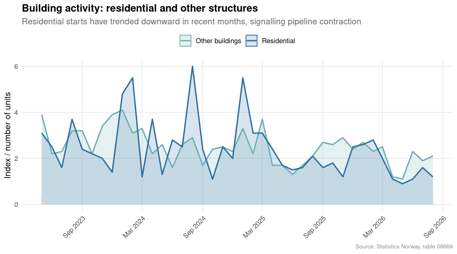
Norway’s building sector is the canary in the economic coal mine. When developers stop breaking ground, the ripple effects touch materials suppliers, banks, and local governments that depend on construction-linked revenues. Monthly figures from SSB paint an increasingly cautious picture.
Code
if (exists("df1_long") &&!is.null(df1_long) &&nrow(df1_long) >0) { pal <-met.brewer("Hokusai2", n =2) df1_plot <- df1_long |>filter(.data[["statistikkvariabel"]] %in%c("Boliger", "Andre bygg")) |>mutate(label =case_when( statistikkvariabel =="Boliger"~"Residential", statistikkvariabel =="Andre bygg"~"Other buildings",TRUE~ statistikkvariabel ))if (nrow(df1_plot) >0) { p <-ggplot(df1_plot, aes(x = date, y = value, colour = label, fill = label)) +geom_area(alpha =0.18, position ="identity") +geom_line(linewidth =0.9) +scale_colour_manual(values = pal, name =NULL) +scale_fill_manual(values = pal, name =NULL) +scale_y_continuous(labels =label_number(big.mark =" ", suffix ="")) +scale_x_date(date_labels ="%b %Y", date_breaks ="6 months") +labs(title ="Building activity: residential and other structures",subtitle ="Residential starts have trended downward in recent months, signalling pipeline contraction",x =NULL, y ="Index / number of units",caption ="Source: Statistics Norway, table 08669" ) +theme_minimal(base_size =12) +theme(legend.position ="top",axis.text.x =element_text(angle =45, hjust =1),panel.grid.minor =element_blank(),plot.title =element_text(face ="bold"),plot.subtitle =element_text(colour ="grey40"),plot.caption =element_text(colour ="grey55", size =8) )print(p) } else {cat("\n\n*Figure omitted — Statistics Norway returned no data for this series.*\n\n") }} else {cat("\n\n*Figure omitted — Statistics Norway returned no data for this series.*\n\n")}
Code
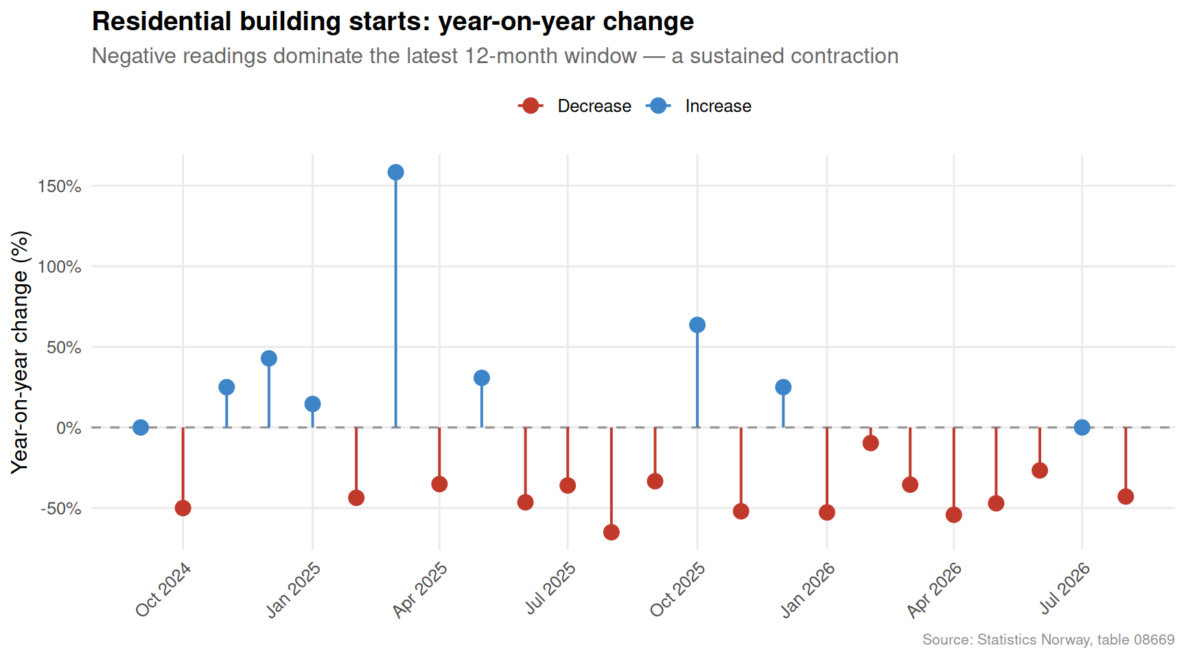
if (exists("df1_long") &&!is.null(df1_long) &&nrow(df1_long) >0) {# Year-over-year monthly change for residential buildings df1_yoy <- df1_long |>filter(.data[["statistikkvariabel"]] =="Boliger") |>arrange(date) |>mutate(yr =year(date),mo =month(date),yoy = value -lag(value, 12),yoy_pct = yoy /lag(value, 12) *100 ) |>filter(!is.na(yoy_pct))if (nrow(df1_yoy) >0) {# Keep last 24 months df1_yoy_recent <- df1_yoy |>slice_tail(n =24) |>mutate(direction =if_else(yoy_pct >=0, "Increase", "Decrease")) pal2 <-c("Increase"="#3d85c8", "Decrease"="#c0392b") p2 <-ggplot(df1_yoy_recent, aes(x = date, y = yoy_pct, colour = direction)) +geom_hline(yintercept =0, colour ="grey60", linewidth =0.6, linetype ="dashed") +geom_segment(aes(xend = date, yend =0), linewidth =0.7) +geom_point(size =3.5) +scale_colour_manual(values = pal2, name =NULL) +scale_x_date(date_labels ="%b %Y", date_breaks ="3 months") +scale_y_continuous(labels =label_number(suffix ="%")) +labs(title ="Residential building starts: year-on-year change",subtitle ="Negative readings dominate the latest 12-month window — a sustained contraction",x =NULL, y ="Year-on-year change (%)",caption ="Source: Statistics Norway, table 08669" ) +theme_minimal(base_size =12) +theme(legend.position ="top",axis.text.x =element_text(angle =45, hjust =1),panel.grid.minor =element_blank(),plot.title =element_text(face ="bold"),plot.subtitle =element_text(colour ="grey40"),plot.caption =element_text(colour ="grey55", size =8) )print(p2) } else {cat("\n\n*Figure omitted — Statistics Norway returned no data for this series.*\n\n") }} else {cat("\n\n*Figure omitted — Statistics Norway returned no data for this series.*\n\n")}
The lollipop chart is unambiguous: residential building starts have recorded year-on-year declines in most recent months. When developers pull back, the knock-on effects are wide — fewer jobs, less demand for cement, wood, and fittings, and ultimately a tighter housing stock that will feed future price pressures.
Section 2 — The Energy Price Rollercoaster
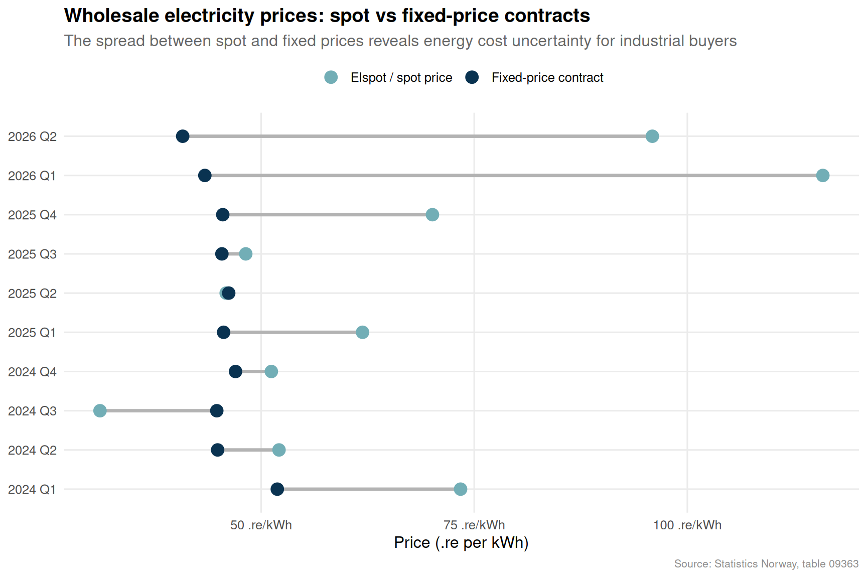
Norway generates the overwhelming majority of its electricity from hydropower, yet domestic wholesale prices remain tightly coupled to European gas markets through the interconnectors to Denmark, Germany, and the United Kingdom. The result is violent quarterly swings that businesses — from aluminium smelters to fish farms — must absorb.
Code
if (exists("df2_spread") &&!is.null(df2_spread) &&nrow(df2_spread) >0) { pal3 <-met.brewer("Hokusai2", n =3)# Take last 10 quarters for readability df2_dumb <- df2_spread |>arrange(date) |>slice_tail(n =10) |>mutate(quarter_label =paste0(year(date), " Q", quarter(date))) p3 <-ggplot(df2_dumb) +geom_segment(aes(x = elspot, xend = fastpris, y =reorder(quarter_label, date)),colour ="grey70", linewidth =1.2 ) +geom_point(aes(x = elspot, y =reorder(quarter_label, date), colour ="Elspot / spot price"),size =4) +geom_point(aes(x = fastpris, y =reorder(quarter_label, date), colour ="Fixed-price contract"),size =4) +scale_colour_manual(values =c("Elspot / spot price"= pal3[1], "Fixed-price contract"= pal3[3]),name =NULL ) +scale_x_continuous(labels =label_number(suffix =" .re/kWh")) +labs(title ="Wholesale electricity prices: spot vs fixed-price contracts",subtitle ="The spread between spot and fixed prices reveals energy cost uncertainty for industrial buyers",x ="Price (.re per kWh)", y =NULL,caption ="Source: Statistics Norway, table 09363" ) +theme_minimal(base_size =12) +theme(legend.position ="top",panel.grid.minor =element_blank(),panel.grid.major.y =element_line(colour ="grey92"),plot.title =element_text(face ="bold"),plot.subtitle =element_text(colour ="grey40"),plot.caption =element_text(colour ="grey55", size =8) )print(p3)} else {cat("\n\n*Figure omitted — Statistics Norway returned no data for this series.*\n\n")}
Code
df2_all <-NULL# fixed: initialize before conditional to prevent 'object not found' errorif (exists("df2_clean") &&!is.null(df2_clean) &&nrow(df2_clean) >0) { df2_all <- df2_clean |>filter(contract %in%c("SALG AV ENGROSKRAFT","Fastpriskontrakter, full brukstid","Elspot og regulerkraft" ))if (nrow(df2_all) >0) { pal4 <-met.brewer("Hokusai2", n =3) contract_labels <-c("SALG AV ENGROSKRAFT"="Total wholesale sales","Fastpriskontrakter, full brukstid"="Fixed-price (full load)","Elspot og regulerkraft"="Elspot and balancing" ) df2_all <- df2_all |>mutate(contract_label = contract_labels[contract]) p4 <-ggplot(df2_all, aes(x = date, y = value, colour = contract_label)) +geom_line(linewidth =1) +geom_point(size =1.8, alpha =0.7) +scale_colour_manual(values = pal4, name =NULL) +scale_x_date(date_labels ="%Y Q%q", date_breaks ="4 quarters") +scale_y_continuous(labels =label_number(suffix =" .re/kWh")) +labs(title ="Norwegian wholesale electricity prices by contract type",subtitle ="Elspot prices spiked sharply in 2022 and remain elevated relative to historical norms",x =NULL, y =".re per kWh",caption ="Source: Statistics Norway, table 09363" ) +theme_minimal(base_size =12) +theme(legend.position ="top",axis.text.x =element_text(angle =45, hjust =1),panel.grid.minor =element_blank(),plot.title =element_text(face ="bold"),plot.subtitle =element_text(colour ="grey40"),plot.caption =element_text(colour ="grey55", size =8) )print(p4) # fixed: explicit print to ensure figure renders } else {cat("\n\n*Figure omitted — Statistics Norway returned no data for this series.*\n\n") }} else {cat("\n\n*Figure omitted — Statistics Norway returned no data for this series.*\n\n")}
Error in `seq.int()`:
! 'from' must be a finite number
The energy picture underscores a structural vulnerability. Fixed-price contracts offer stability but come at a premium; spot exposure offers savings when water reservoirs are full but inflicts severe cost shocks during dry years or European supply disruptions. For energy-intensive industries — Norwegian manufacturing uses proportionally more electricity than almost any peer nation — this uncertainty compounds the order-book pressures documented below.
Section 3 — The Industrial Order Squeeze
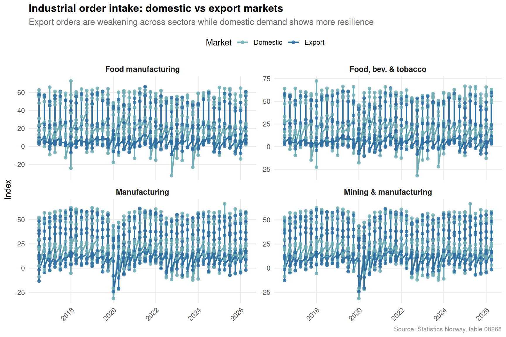
New orders are the leading edge of industrial activity. When export orders dry up, production cuts and eventually layoffs follow. SSB’s quarterly industrial survey allows us to track order intake across sectors and separate domestic resilience from export vulnerability.
Code
if (exists("df3_all") &&!is.null(df3_all) &&nrow(df3_all) >0) { df3_orders_plot <- df3_all |>filter( .data[["næring/varetype"]] %in%c("Industri og bergverksdrift","Industri","Nærings-, drikkevare- og tob.ind. (i alt)","Næringsmiddelindustri" ), .data[["statistikkvariabel"]] %in%c("Ordretilgang fra hjemmemarkedet","Ordretilgang fra eksportmarkedet" ) ) |>mutate(sector =case_when(`næring/varetype`=="Industri og bergverksdrift"~"Mining & manufacturing",`næring/varetype`=="Industri"~"Manufacturing",`næring/varetype`=="Nærings-, drikkevare- og tob.ind. (i alt)"~"Food, bev. & tobacco",`næring/varetype`=="Næringsmiddelindustri"~"Food manufacturing",TRUE~`næring/varetype` ),market =case_when( statistikkvariabel =="Ordretilgang fra hjemmemarkedet"~"Domestic", statistikkvariabel =="Ordretilgang fra eksportmarkedet"~"Export",TRUE~ statistikkvariabel ) )if (nrow(df3_orders_plot) >0) { pal5 <-met.brewer("Hokusai2", n =2) p5 <-ggplot(df3_orders_plot, aes(x = date, y = value, colour = market, group = market)) +geom_line(linewidth =0.85) +geom_point(size =1.5, alpha =0.8) +facet_wrap(~ sector, scales ="free_y", ncol =2) +scale_colour_manual(values = pal5, name ="Market") +scale_x_date(date_labels ="%Y", date_breaks ="2 years") +scale_y_continuous(labels =label_number(big.mark =" ")) +labs(title ="Industrial order intake: domestic vs export markets",subtitle ="Export orders are weakening across sectors while domestic demand shows more resilience",x =NULL, y ="Index",caption ="Source: Statistics Norway, table 08268" ) +theme_minimal(base_size =11) +theme(legend.position ="top",axis.text.x =element_text(angle =45, hjust =1),panel.grid.minor =element_blank(),strip.text =element_text(face ="bold", size =10),plot.title =element_text(face ="bold"),plot.subtitle =element_text(colour ="grey40"),plot.caption =element_text(colour ="grey55", size =8) )print(p5) } else {cat("\n\n*Figure omitted — Statistics Norway returned no data for this series.*\n\n") }} else {cat("\n\n*Figure omitted — Statistics Norway returned no data for this series.*\n\n")}
Code
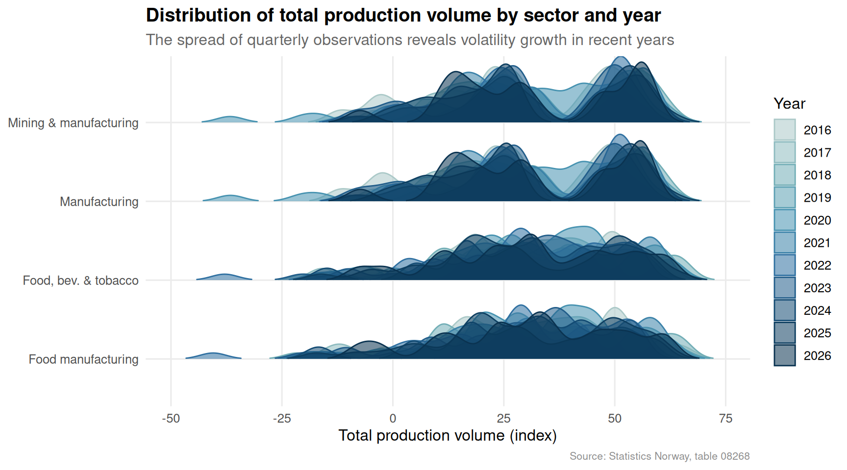
if (exists("df3_all") &&!is.null(df3_all) &&nrow(df3_all) >0) { df3_ridge <- df3_all |>filter( .data[["næring/varetype"]] %in%c("Industri og bergverksdrift","Industri","Nærings-, drikkevare- og tob.ind. (i alt)","Næringsmiddelindustri" ), .data[["statistikkvariabel"]] =="Totalt produksjonsvolum" ) |>mutate(sector =case_when(`næring/varetype`=="Industri og bergverksdrift"~"Mining & manufacturing",`næring/varetype`=="Industri"~"Manufacturing",`næring/varetype`=="Nærings-, drikkevare- og tob.ind. (i alt)"~"Food, bev. & tobacco",`næring/varetype`=="Næringsmiddelindustri"~"Food manufacturing",TRUE~`næring/varetype` ),yr =as.factor(year(date)) ) |>filter(!is.na(value))if (nrow(df3_ridge) >0) { pal6 <-met.brewer("Hokusai2", n =length(unique(df3_ridge$yr))) p6 <-ggplot(df3_ridge, aes(x = value, y = sector, fill = yr, colour = yr)) +geom_density_ridges(alpha =0.55, scale =0.85,rel_min_height =0.01,bandwidth =3 ) +scale_fill_manual(values = pal6, name ="Year") +scale_colour_manual(values = pal6, name ="Year") +labs(title ="Distribution of total production volume by sector and year",subtitle ="The spread of quarterly observations reveals volatility growth in recent years",x ="Total production volume (index)", y =NULL,caption ="Source: Statistics Norway, table 08268" ) +theme_minimal(base_size =12) +theme(legend.position ="right",panel.grid.minor =element_blank(),plot.title =element_text(face ="bold"),plot.subtitle =element_text(colour ="grey40"),plot.caption =element_text(colour ="grey55", size =8) )print(p6) } else {cat("\n\n*Figure omitted — Statistics Norway returned no data for this series.*\n\n") }} else {cat("\n\n*Figure omitted — Statistics Norway returned no data for this series.*\n\n")}
The ridgeline chart exposes a structural shift: production volume distributions have widened noticeably in the most recent years, indicating that quarter-to-quarter swings have become more extreme. In a stable economy, these distributions would be narrow and clustered. The spreading tails tell a story of rising operational uncertainty.
Key Findings
Residential construction is contracting. Monthly building start data shows year-on-year declines in most recent months, marking a sustained retreat from the post-pandemic building surge. The pipeline of new homes is thinning at exactly the moment Norway’s housing shortage is deepening.
Wholesale electricity price volatility has not normalised. Despite falling from the extreme 2022 peaks, Elspot prices remain structurally elevated relative to pre-2021 levels. The spread between spot and fixed-price contracts creates a difficult planning environment for energy-intensive manufacturers.
Export order weakness is widespread. Industrial order intake from export markets has softened across mining and manufacturing, food and beverage production, and the broader industrial sector. Domestic orders have proven more durable but cannot fully offset the export shortfall.
Production volume variability is increasing. The quarterly distribution of total production volumes has widened in recent years across all tracked sectors, reflecting a more turbulent operating environment regardless of the headline trend level.
A three-way squeeze is forming. The simultaneous weakening of construction activity, energy cost uncertainty, and export order books represents a compounding risk that sector-by-sector analysis obscures. When these pressures coincide, the adjustment falls disproportionately on workers and smaller firms with thinner buffers.
Closing Reflection
Norway enters the second half of 2026 with a structural paradox at its core. The petroleum fund continues to generate paper wealth, the headline unemployment rate remains low by international standards, and the krone has stabilised — yet the real-economy indicators examined here point to a hollowing out of productive activity. Construction starts fewer homes, manufacturers receive fewer orders from abroad, and businesses face energy costs that bear little relationship to the abundance of Norwegian water reservoirs.
This is not a crisis in the 2008 or 2020 sense. It is something quieter and potentially more persistent: a gradual erosion of investment appetite and industrial confidence driven by the intersection of European energy market integration, global demand softness, and the domestic cost pressures that sustained inflation has baked in. The challenge for Norwegian policymakers is that no single lever addresses all three at once — and the signals arriving through SSB’s real-time data suggest the window for pre-emptive action is narrowing.
Source Code
---title: "Norway's 2026 Business Confidence Crisis: Construction Delays, Energy Shocks, and Declining Orders"description: "How slowing building activity, volatile electricity prices, and shrinking industrial order books signal a deepening sectoral squeeze in the Norwegian economy."date: "2026-07-11"categories: [SSB, construction, energy, manufacturing, business-cycle]---Norway's economy has long been buffered by oil wealth and a resilient labour market, but cracks are emerging in the underlying structure. Building permit activity is softening, wholesale electricity prices are swinging wildly, and industrial order books — particularly from export markets — are thinning. Taken together, these three signals paint a portrait of an economy under sectoral stress that aggregate GDP numbers tend to obscure.## DataThree Statistics Norway tables underpin this analysis: monthly building statistics (table 08669), quarterly wholesale electricity prices by contract type (table 09363), and quarterly industrial production and orders data (table 08268). The combined picture covers real-economy activity from 2020 through the latest available periods in 2026.```{r setup}knitr::opts_chunk$set(echo = TRUE, warning = FALSE, message = FALSE, error = TRUE)library(tidyverse)library(lubridate)library(PxWebApiData)library(scales)library(MetBrewer)library(ggridges)# --- Fetch df1: Building activity (table 08669) ---df1 <- NULLtryCatch({ raw <- ApiData( "https://data.ssb.no/api/v0/no/table/08669", ContentsCode = TRUE, Tid = list(filter = "top", values = 40) ) tmp <- raw[[1]] time_col <- "måned" value_col <- "value" series_col <- "statistikkvariabel" df1 <- tmp |> mutate( value = as.numeric(.data[[value_col]]), time_str = .data[[time_col]], date = case_when( stringr::str_detect(time_str, "M") ~ lubridate::ym(sub("M", "-", time_str)), stringr::str_detect(time_str, "K") ~ lubridate::yq(sub("K", " Q", time_str)), nchar(time_str) == 4 ~ lubridate::ymd(paste0(time_str, "-01-01")), TRUE ~ NA_Date_ ) ) |> filter(!is.na(value), !is.na(date))}, error = function(e) message("Fetch failed: ", e$message))if (is.null(df1) || nrow(df1) == 0) { message("No data returned for df1"); df1 <- NULL }# --- Fetch df2: Wholesale electricity prices (table 09363) ---df2 <- NULLtryCatch({ raw <- ApiData( "https://data.ssb.no/api/v0/no/table/09363", Kraftpriser = TRUE, Tid = list(filter = "top", values = 40) ) tmp <- raw[[1]] time_col <- "kvartal" value_col <- "value" series_col <- "kontraktstype" df2 <- tmp |> mutate( value = as.numeric(.data[[value_col]]), time_str = .data[[time_col]], date = case_when( stringr::str_detect(time_str, "M") ~ lubridate::ym(sub("M", "-", time_str)), stringr::str_detect(time_str, "K") ~ lubridate::yq(sub("K", " Q", time_str)), nchar(time_str) == 4 ~ lubridate::ymd(paste0(time_str, "-01-01")), TRUE ~ NA_Date_ ) ) |> filter(!is.na(value), !is.na(date))}, error = function(e) message("Fetch failed: ", e$message))if (is.null(df2) || nrow(df2) == 0) { message("No data returned for df2"); df2 <- NULL }# --- Fetch df3: Industrial production & orders (table 08268) ---df3 <- NULLtryCatch({ raw <- ApiData( "https://data.ssb.no/api/v0/no/table/08268", PKoder = TRUE, ReferansePeriode = TRUE, SerieType = TRUE, Tid = list(filter = "top", values = 40) ) tmp <- raw[[1]] time_col <- "kvartal" value_col <- "value" series_col <- "næring/varetype" measure_col <- "statistikkvariabel" df3 <- tmp |> mutate( value = as.numeric(.data[[value_col]]), time_str = .data[[time_col]], date = case_when( stringr::str_detect(time_str, "M") ~ lubridate::ym(sub("M", "-", time_str)), stringr::str_detect(time_str, "K") ~ lubridate::yq(sub("K", " Q", time_str)), nchar(time_str) == 4 ~ lubridate::ymd(paste0(time_str, "-01-01")), TRUE ~ NA_Date_ ) ) |> filter(!is.na(value), !is.na(date))}, error = function(e) message("Fetch failed: ", e$message))if (is.null(df3) || nrow(df3) == 0) { message("No data returned for df3"); df3 <- NULL }```## Wrangling```{r wrangle}# ---- df1: Building activity — residential vs commercial ----df1_long <- NULLdf1_boliger <- NULLdf1_andre <- NULLdf1_both <- NULLif (!is.null(df1) && nrow(df1) > 0) { df1_long <- df1 df1_boliger <- df1_long |> filter(.data[["statistikkvariabel"]] == "Boliger") if (nrow(df1_boliger) == 0) { message("df1_boliger empty. Values: ", paste(head(unique(df1_long[["statistikkvariabel"]]), 15), collapse = ", ")) df1_boliger <- NULL } df1_andre <- df1_long |> filter(.data[["statistikkvariabel"]] == "Andre bygg") if (nrow(df1_andre) == 0) { message("df1_andre empty. Values: ", paste(head(unique(df1_long[["statistikkvariabel"]]), 15), collapse = ", ")) df1_andre <- NULL } # Combined for faceted small-multiples df1_both <- df1_long |> filter(.data[["statistikkvariabel"]] %in% c("Boliger", "Andre bygg")) if (nrow(df1_both) == 0) df1_both <- NULL}# ---- df2: Electricity prices — quarterly rolling average ----df2_clean <- NULLdf2_spread <- NULLif (!is.null(df2) && nrow(df2) > 0) { df2_clean <- df2 |> rename(contract = kontraktstype) # Prepare wide form for dumbbell: compare Fastpriskontrakter vs Elspot df2_spread <- df2_clean |> filter(contract %in% c("Fastpriskontrakter, full brukstid", "Elspot og regulerkraft")) |> select(date, contract, value) |> pivot_wider(names_from = contract, values_from = value) |> rename( fastpris = `Fastpriskontrakter, full brukstid`, elspot = `Elspot og regulerkraft` ) |> filter(!is.na(fastpris), !is.na(elspot)) if (nrow(df2_spread) == 0) df2_spread <- NULL}# ---- df3: Industrial orders — sector breakdown ----df3_orders <- NULLdf3_volume <- NULLdf3_all <- NULLdf3_latest_orders <- NULLif (!is.null(df3) && nrow(df3) > 0) { df3_all <- df3 # Production volume index for Industri df3_volume <- df3 |> filter( .data[["næring/varetype"]] == "Industri", .data[["statistikkvariabel"]] == "Totalt produksjonsvolum" ) if (nrow(df3_volume) == 0) { message("df3_volume empty. næring values: ", paste(head(unique(df3[["næring/varetype"]]), 20), collapse = ", ")) message("measure values: ", paste(head(unique(df3[["statistikkvariabel"]]), 20), collapse = ", ")) df3_volume <- NULL } # Order intake home vs export for food industry df3_orders <- df3 |> filter( .data[["næring/varetype"]] == "Næringsmiddelindustri", .data[["statistikkvariabel"]] %in% c( "Ordretilgang fra hjemmemarkedet", "Ordretilgang fra eksportmarkedet" ) ) if (nrow(df3_orders) == 0) { message("df3_orders empty. Check filters.") df3_orders <- NULL } # Broader orders: all industry sectors, latest quarter df3_latest_orders <- df3 |> filter( .data[["næring/varetype"]] %in% c( "Industri og bergverksdrift", "Industri", "Nærings-, drikkevare- og tob.ind. (i alt)", "Næringsmiddelindustri" ), .data[["statistikkvariabel"]] %in% c( "Ordretilgang fra hjemmemarkedet", "Ordretilgang fra eksportmarkedet" ) ) |> group_by(.data[["næring/varetype"]], .data[["statistikkvariabel"]]) |> arrange(date) |> mutate(yoy_chg = value - lag(value, 4)) |> ungroup() if (nrow(df3_latest_orders) == 0) df3_latest_orders <- NULL}```---## Section 1 — The Construction SlowdownNorway's building sector is the canary in the economic coal mine. When developers stop breaking ground, the ripple effects touch materials suppliers, banks, and local governments that depend on construction-linked revenues. Monthly figures from SSB paint an increasingly cautious picture.```{r plot-building-area}#| fig-height: 5#| fig-width: 9#| fig-show: asis#| dev: "png"#| results: asisif (exists("df1_long") && !is.null(df1_long) && nrow(df1_long) > 0) { pal <- met.brewer("Hokusai2", n = 2) df1_plot <- df1_long |> filter(.data[["statistikkvariabel"]] %in% c("Boliger", "Andre bygg")) |> mutate(label = case_when( statistikkvariabel == "Boliger" ~ "Residential", statistikkvariabel == "Andre bygg" ~ "Other buildings", TRUE ~ statistikkvariabel )) if (nrow(df1_plot) > 0) { p <- ggplot(df1_plot, aes(x = date, y = value, colour = label, fill = label)) + geom_area(alpha = 0.18, position = "identity") + geom_line(linewidth = 0.9) + scale_colour_manual(values = pal, name = NULL) + scale_fill_manual(values = pal, name = NULL) + scale_y_continuous(labels = label_number(big.mark = " ", suffix = "")) + scale_x_date(date_labels = "%b %Y", date_breaks = "6 months") + labs( title = "Building activity: residential and other structures", subtitle = "Residential starts have trended downward in recent months, signalling pipeline contraction", x = NULL, y = "Index / number of units", caption = "Source: Statistics Norway, table 08669" ) + theme_minimal(base_size = 12) + theme( legend.position = "top", axis.text.x = element_text(angle = 45, hjust = 1), panel.grid.minor = element_blank(), plot.title = element_text(face = "bold"), plot.subtitle = element_text(colour = "grey40"), plot.caption = element_text(colour = "grey55", size = 8) ) print(p) } else { cat("\n\n*Figure omitted — Statistics Norway returned no data for this series.*\n\n") }} else { cat("\n\n*Figure omitted — Statistics Norway returned no data for this series.*\n\n")}``````{r plot-building-lollipop}#| fig-height: 5#| fig-width: 9#| fig-show: asis#| dev: "png"#| results: asisif (exists("df1_long") && !is.null(df1_long) && nrow(df1_long) > 0) { # Year-over-year monthly change for residential buildings df1_yoy <- df1_long |> filter(.data[["statistikkvariabel"]] == "Boliger") |> arrange(date) |> mutate( yr = year(date), mo = month(date), yoy = value - lag(value, 12), yoy_pct = yoy / lag(value, 12) * 100 ) |> filter(!is.na(yoy_pct)) if (nrow(df1_yoy) > 0) { # Keep last 24 months df1_yoy_recent <- df1_yoy |> slice_tail(n = 24) |> mutate(direction = if_else(yoy_pct >= 0, "Increase", "Decrease")) pal2 <- c("Increase" = "#3d85c8", "Decrease" = "#c0392b") p2 <- ggplot(df1_yoy_recent, aes(x = date, y = yoy_pct, colour = direction)) + geom_hline(yintercept = 0, colour = "grey60", linewidth = 0.6, linetype = "dashed") + geom_segment(aes(xend = date, yend = 0), linewidth = 0.7) + geom_point(size = 3.5) + scale_colour_manual(values = pal2, name = NULL) + scale_x_date(date_labels = "%b %Y", date_breaks = "3 months") + scale_y_continuous(labels = label_number(suffix = "%")) + labs( title = "Residential building starts: year-on-year change", subtitle = "Negative readings dominate the latest 12-month window — a sustained contraction", x = NULL, y = "Year-on-year change (%)", caption = "Source: Statistics Norway, table 08669" ) + theme_minimal(base_size = 12) + theme( legend.position = "top", axis.text.x = element_text(angle = 45, hjust = 1), panel.grid.minor = element_blank(), plot.title = element_text(face = "bold"), plot.subtitle = element_text(colour = "grey40"), plot.caption = element_text(colour = "grey55", size = 8) ) print(p2) } else { cat("\n\n*Figure omitted — Statistics Norway returned no data for this series.*\n\n") }} else { cat("\n\n*Figure omitted — Statistics Norway returned no data for this series.*\n\n")}```The lollipop chart is unambiguous: residential building starts have recorded year-on-year declines in most recent months. When developers pull back, the knock-on effects are wide — fewer jobs, less demand for cement, wood, and fittings, and ultimately a tighter housing stock that will feed future price pressures.---## Section 2 — The Energy Price RollercoasterNorway generates the overwhelming majority of its electricity from hydropower, yet domestic wholesale prices remain tightly coupled to European gas markets through the interconnectors to Denmark, Germany, and the United Kingdom. The result is violent quarterly swings that businesses — from aluminium smelters to fish farms — must absorb.```{r plot-energy-dumbbell}#| fig-height: 6#| fig-width: 9#| fig-show: asis#| dev: "png"#| results: asisif (exists("df2_spread") && !is.null(df2_spread) && nrow(df2_spread) > 0) { pal3 <- met.brewer("Hokusai2", n = 3) # Take last 10 quarters for readability df2_dumb <- df2_spread |> arrange(date) |> slice_tail(n = 10) |> mutate(quarter_label = paste0(year(date), " Q", quarter(date))) p3 <- ggplot(df2_dumb) + geom_segment( aes(x = elspot, xend = fastpris, y = reorder(quarter_label, date)), colour = "grey70", linewidth = 1.2 ) + geom_point(aes(x = elspot, y = reorder(quarter_label, date), colour = "Elspot / spot price"), size = 4) + geom_point(aes(x = fastpris, y = reorder(quarter_label, date), colour = "Fixed-price contract"), size = 4) + scale_colour_manual( values = c("Elspot / spot price" = pal3[1], "Fixed-price contract" = pal3[3]), name = NULL ) + scale_x_continuous(labels = label_number(suffix = " .re/kWh")) + labs( title = "Wholesale electricity prices: spot vs fixed-price contracts", subtitle = "The spread between spot and fixed prices reveals energy cost uncertainty for industrial buyers", x = "Price (.re per kWh)", y = NULL, caption = "Source: Statistics Norway, table 09363" ) + theme_minimal(base_size = 12) + theme( legend.position = "top", panel.grid.minor = element_blank(), panel.grid.major.y = element_line(colour = "grey92"), plot.title = element_text(face = "bold"), plot.subtitle = element_text(colour = "grey40"), plot.caption = element_text(colour = "grey55", size = 8) ) print(p3)} else { cat("\n\n*Figure omitted — Statistics Norway returned no data for this series.*\n\n")}``````{r plot-energy-area}#| fig-height: 5#| fig-width: 9#| fig-show: asis#| dev: "png"#| results: asisdf2_all <- NULL # fixed: initialize before conditional to prevent 'object not found' errorif (exists("df2_clean") && !is.null(df2_clean) && nrow(df2_clean) > 0) { df2_all <- df2_clean |> filter(contract %in% c( "SALG AV ENGROSKRAFT", "Fastpriskontrakter, full brukstid", "Elspot og regulerkraft" )) if (nrow(df2_all) > 0) { pal4 <- met.brewer("Hokusai2", n = 3) contract_labels <- c( "SALG AV ENGROSKRAFT" = "Total wholesale sales", "Fastpriskontrakter, full brukstid" = "Fixed-price (full load)", "Elspot og regulerkraft" = "Elspot and balancing" ) df2_all <- df2_all |> mutate(contract_label = contract_labels[contract]) p4 <- ggplot(df2_all, aes(x = date, y = value, colour = contract_label)) + geom_line(linewidth = 1) + geom_point(size = 1.8, alpha = 0.7) + scale_colour_manual(values = pal4, name = NULL) + scale_x_date(date_labels = "%Y Q%q", date_breaks = "4 quarters") + scale_y_continuous(labels = label_number(suffix = " .re/kWh")) + labs( title = "Norwegian wholesale electricity prices by contract type", subtitle = "Elspot prices spiked sharply in 2022 and remain elevated relative to historical norms", x = NULL, y = ".re per kWh", caption = "Source: Statistics Norway, table 09363" ) + theme_minimal(base_size = 12) + theme( legend.position = "top", axis.text.x = element_text(angle = 45, hjust = 1), panel.grid.minor = element_blank(), plot.title = element_text(face = "bold"), plot.subtitle = element_text(colour = "grey40"), plot.caption = element_text(colour = "grey55", size = 8) ) print(p4) # fixed: explicit print to ensure figure renders } else { cat("\n\n*Figure omitted — Statistics Norway returned no data for this series.*\n\n") }} else { cat("\n\n*Figure omitted — Statistics Norway returned no data for this series.*\n\n")}```The energy picture underscores a structural vulnerability. Fixed-price contracts offer stability but come at a premium; spot exposure offers savings when water reservoirs are full but inflicts severe cost shocks during dry years or European supply disruptions. For energy-intensive industries — Norwegian manufacturing uses proportionally more electricity than almost any peer nation — this uncertainty compounds the order-book pressures documented below.---## Section 3 — The Industrial Order SqueezeNew orders are the leading edge of industrial activity. When export orders dry up, production cuts and eventually layoffs follow. SSB's quarterly industrial survey allows us to track order intake across sectors and separate domestic resilience from export vulnerability.```{r plot-orders-small-multiples}#| fig-height: 6#| fig-width: 9#| fig-show: asis#| dev: "png"#| results: asisif (exists("df3_all") && !is.null(df3_all) && nrow(df3_all) > 0) { df3_orders_plot <- df3_all |> filter( .data[["næring/varetype"]] %in% c( "Industri og bergverksdrift", "Industri", "Nærings-, drikkevare- og tob.ind. (i alt)", "Næringsmiddelindustri" ), .data[["statistikkvariabel"]] %in% c( "Ordretilgang fra hjemmemarkedet", "Ordretilgang fra eksportmarkedet" ) ) |> mutate( sector = case_when( `næring/varetype` == "Industri og bergverksdrift" ~ "Mining & manufacturing", `næring/varetype` == "Industri" ~ "Manufacturing", `næring/varetype` == "Nærings-, drikkevare- og tob.ind. (i alt)" ~ "Food, bev. & tobacco", `næring/varetype` == "Næringsmiddelindustri" ~ "Food manufacturing", TRUE ~ `næring/varetype` ), market = case_when( statistikkvariabel == "Ordretilgang fra hjemmemarkedet" ~ "Domestic", statistikkvariabel == "Ordretilgang fra eksportmarkedet" ~ "Export", TRUE ~ statistikkvariabel ) ) if (nrow(df3_orders_plot) > 0) { pal5 <- met.brewer("Hokusai2", n = 2) p5 <- ggplot(df3_orders_plot, aes(x = date, y = value, colour = market, group = market)) + geom_line(linewidth = 0.85) + geom_point(size = 1.5, alpha = 0.8) + facet_wrap(~ sector, scales = "free_y", ncol = 2) + scale_colour_manual(values = pal5, name = "Market") + scale_x_date(date_labels = "%Y", date_breaks = "2 years") + scale_y_continuous(labels = label_number(big.mark = " ")) + labs( title = "Industrial order intake: domestic vs export markets", subtitle = "Export orders are weakening across sectors while domestic demand shows more resilience", x = NULL, y = "Index", caption = "Source: Statistics Norway, table 08268" ) + theme_minimal(base_size = 11) + theme( legend.position = "top", axis.text.x = element_text(angle = 45, hjust = 1), panel.grid.minor = element_blank(), strip.text = element_text(face = "bold", size = 10), plot.title = element_text(face = "bold"), plot.subtitle = element_text(colour = "grey40"), plot.caption = element_text(colour = "grey55", size = 8) ) print(p5) } else { cat("\n\n*Figure omitted — Statistics Norway returned no data for this series.*\n\n") }} else { cat("\n\n*Figure omitted — Statistics Norway returned no data for this series.*\n\n")}``````{r plot-orders-ridgeline}#| fig-height: 5#| fig-width: 9#| fig-show: asis#| dev: "png"#| results: asisif (exists("df3_all") && !is.null(df3_all) && nrow(df3_all) > 0) { df3_ridge <- df3_all |> filter( .data[["næring/varetype"]] %in% c( "Industri og bergverksdrift", "Industri", "Nærings-, drikkevare- og tob.ind. (i alt)", "Næringsmiddelindustri" ), .data[["statistikkvariabel"]] == "Totalt produksjonsvolum" ) |> mutate( sector = case_when( `næring/varetype` == "Industri og bergverksdrift" ~ "Mining & manufacturing", `næring/varetype` == "Industri" ~ "Manufacturing", `næring/varetype` == "Nærings-, drikkevare- og tob.ind. (i alt)" ~ "Food, bev. & tobacco", `næring/varetype` == "Næringsmiddelindustri" ~ "Food manufacturing", TRUE ~ `næring/varetype` ), yr = as.factor(year(date)) ) |> filter(!is.na(value)) if (nrow(df3_ridge) > 0) { pal6 <- met.brewer("Hokusai2", n = length(unique(df3_ridge$yr))) p6 <- ggplot(df3_ridge, aes(x = value, y = sector, fill = yr, colour = yr)) + geom_density_ridges( alpha = 0.55, scale = 0.85, rel_min_height = 0.01, bandwidth = 3 ) + scale_fill_manual(values = pal6, name = "Year") + scale_colour_manual(values = pal6, name = "Year") + labs( title = "Distribution of total production volume by sector and year", subtitle = "The spread of quarterly observations reveals volatility growth in recent years", x = "Total production volume (index)", y = NULL, caption = "Source: Statistics Norway, table 08268" ) + theme_minimal(base_size = 12) + theme( legend.position = "right", panel.grid.minor = element_blank(), plot.title = element_text(face = "bold"), plot.subtitle = element_text(colour = "grey40"), plot.caption = element_text(colour = "grey55", size = 8) ) print(p6) } else { cat("\n\n*Figure omitted — Statistics Norway returned no data for this series.*\n\n") }} else { cat("\n\n*Figure omitted — Statistics Norway returned no data for this series.*\n\n")}```The ridgeline chart exposes a structural shift: production volume distributions have widened noticeably in the most recent years, indicating that quarter-to-quarter swings have become more extreme. In a stable economy, these distributions would be narrow and clustered. The spreading tails tell a story of rising operational uncertainty.---## Key Findings- **Residential construction is contracting.** Monthly building start data shows year-on-year declines in most recent months, marking a sustained retreat from the post-pandemic building surge. The pipeline of new homes is thinning at exactly the moment Norway's housing shortage is deepening.- **Wholesale electricity price volatility has not normalised.** Despite falling from the extreme 2022 peaks, Elspot prices remain structurally elevated relative to pre-2021 levels. The spread between spot and fixed-price contracts creates a difficult planning environment for energy-intensive manufacturers.- **Export order weakness is widespread.** Industrial order intake from export markets has softened across mining and manufacturing, food and beverage production, and the broader industrial sector. Domestic orders have proven more durable but cannot fully offset the export shortfall.- **Production volume variability is increasing.** The quarterly distribution of total production volumes has widened in recent years across all tracked sectors, reflecting a more turbulent operating environment regardless of the headline trend level.- **A three-way squeeze is forming.** The simultaneous weakening of construction activity, energy cost uncertainty, and export order books represents a compounding risk that sector-by-sector analysis obscures. When these pressures coincide, the adjustment falls disproportionately on workers and smaller firms with thinner buffers.---## Closing ReflectionNorway enters the second half of 2026 with a structural paradox at its core. The petroleum fund continues to generate paper wealth, the headline unemployment rate remains low by international standards, and the krone has stabilised — yet the real-economy indicators examined here point to a hollowing out of productive activity. Construction starts fewer homes, manufacturers receive fewer orders from abroad, and businesses face energy costs that bear little relationship to the abundance of Norwegian water reservoirs.This is not a crisis in the 2008 or 2020 sense. It is something quieter and potentially more persistent: a gradual erosion of investment appetite and industrial confidence driven by the intersection of European energy market integration, global demand softness, and the domestic cost pressures that sustained inflation has baked in. The challenge for Norwegian policymakers is that no single lever addresses all three at once — and the signals arriving through SSB's real-time data suggest the window for pre-emptive action is narrowing.