New dwelling prices have climbed sharply while post-secondary vocational enrolments stagnate, pricing young tradespeople out of the very homes their skills are needed to build.
Published
July 10, 2026
Norway faces a compounding structural problem. The price of new dwellings has risen well ahead of general inflation, yet the pipeline of vocationally trained workers entering the construction and trades sector has barely moved for years. The people most needed to build affordable homes are increasingly priced out of owning one.
# --- Derived data frames: declare all up front ---df1_index <-NULLdf1_yoy <-NULLdf1_all_index <-NULLdf2_total <-NULLdf2_young <-NULLdf2_age_trend <-NULLdf2_gender <-NULL# --- df1 wrangling ---if (!is.null(df1) &&nrow(df1) >0) { df1_index <- df1 |>filter(.data[["statistikkvariabel"]] =="Prisindeks (2015=100)") |>filter(.data[["boligtype"]] %in%c("Alle boligtyper", "Eneboliger", "Flerbolig"))if (nrow(df1_index) ==0) {message("df1_index empty. measure values: ",paste(head(unique(df1[["statistikkvariabel"]]), 10), collapse =", ")) df1_index <-NULL } df1_yoy <- df1 |>filter(.data[["statistikkvariabel"]] =="Prosentvis endring av indeks fra samme kvartal året før") |>filter(.data[["boligtype"]] %in%c("Alle boligtyper", "Eneboliger", "Flerbolig"))if (nrow(df1_yoy) ==0) {message("df1_yoy empty.") df1_yoy <-NULL }# All dwelling types index for area chart df1_all_index <- df1 |>filter(.data[["statistikkvariabel"]] =="Prisindeks (2015=100)", .data[["boligtype"]] =="Alle boligtyper") |>arrange(date)if (nrow(df1_all_index) ==0) { df1_all_index <-NULL }}# --- df2 wrangling ---if (!is.null(df2) &&nrow(df2) >0) {# Total enrolments across all age groups (kjønn = "Begge kjønn" or equivalent)# Check gender column name gender_col <-if ("kjønn"%in%names(df2)) "kjønn"elseif ("kjonn"%in%names(df2)) "kjonn"elseNULL owner_col <-if ("eierforhold"%in%names(df2)) "eierforhold"elseNULL# Total: alder i alt, both genders, all ownership df2_total <- df2 |>filter(.data[["alder"]] =="Alder i alt")if (!is.null(gender_col)) { gender_vals <-unique(df2[[gender_col]]) both_val <- gender_vals[str_detect(tolower(gender_vals), "begge|total|i alt|alle")][1]if (!is.na(both_val)) { df2_total <- df2_total |>filter(.data[[gender_col]] == both_val) } }if (!is.null(owner_col)) { owner_vals <-unique(df2[[owner_col]]) all_val <- owner_vals[str_detect(tolower(owner_vals), "i alt|total|alle|begge")][1]if (!is.na(all_val)) { df2_total <- df2_total |>filter(.data[[owner_col]] == all_val) } } df2_total <- df2_total |>group_by(date, time_str) |>summarise(value =sum(value, na.rm =TRUE), .groups ="drop") |>arrange(date)if (nrow(df2_total) ==0) { df2_total <-NULL }# By age group (excluding "Alder i alt"), both genders, all ownership df2_age_trend <- df2 |>filter(.data[["alder"]] !="Alder i alt")if (!is.null(gender_col)) { gender_vals <-unique(df2[[gender_col]]) both_val <- gender_vals[str_detect(tolower(gender_vals), "begge|total|i alt|alle")][1]if (!is.na(both_val)) { df2_age_trend <- df2_age_trend |>filter(.data[[gender_col]] == both_val) } }if (!is.null(owner_col)) { owner_vals <-unique(df2[[owner_col]]) all_val <- owner_vals[str_detect(tolower(owner_vals), "i alt|total|alle|begge")][1]if (!is.na(all_val)) { df2_age_trend <- df2_age_trend |>filter(.data[[owner_col]] == all_val) } } df2_age_trend <- df2_age_trend |>group_by(date, time_str, alder) |>summarise(value =sum(value, na.rm =TRUE), .groups ="drop") |>arrange(date)if (nrow(df2_age_trend) ==0) { df2_age_trend <-NULL }# Young vs older: 20 or younger + 21-25 vs restif (!is.null(df2_age_trend)) { df2_young <- df2_age_trend |>mutate(group =case_when( alder %in%c("20 år eller yngre", "21-25 år") ~"Under 26",TRUE~"26 og eldre" )) |>group_by(date, time_str, group) |>summarise(value =sum(value, na.rm =TRUE), .groups ="drop")if (nrow(df2_young) ==0) { df2_young <-NULL } }# Gender breakdown: alder i alt, all ownershipif (!is.null(gender_col)) { df2_gender <- df2 |>filter(.data[["alder"]] =="Alder i alt")if (!is.null(owner_col)) { owner_vals <-unique(df2[[owner_col]]) all_val <- owner_vals[str_detect(tolower(owner_vals), "i alt|total|alle|begge")][1]if (!is.na(all_val)) { df2_gender <- df2_gender |>filter(.data[[owner_col]] == all_val) } } df2_gender <- df2_gender |>filter(!str_detect(tolower(.data[[gender_col]]), "begge|total|i alt|alle")) |>group_by(date, time_str, .data[[gender_col]]) |>summarise(value =sum(value, na.rm =TRUE), .groups ="drop") |>rename(gender = .data[[gender_col]]) |>arrange(date)if (nrow(df2_gender) ==0) { df2_gender <-NULL } }}# Colour palettespal_housing <-met.brewer("Hokusai2", n =3)pal_edu <-met.brewer("Derain", n =6)pal_two <-met.brewer("Hokusai2", n =2)
New Dwelling Prices: A Relentless Climb
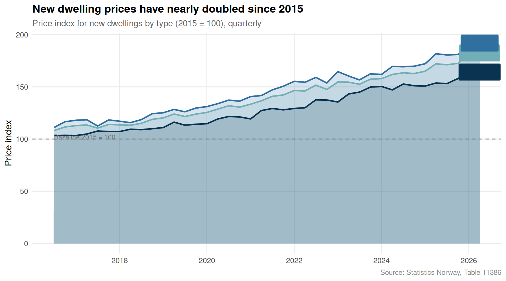
Since Statistics Norway rebased its housing price index to 2015, the index has risen substantially across all dwelling types. Single-family homes and multi-family buildings have followed different trajectories, but both have left the 2015 baseline far behind.
Code
if (exists("df1_index") &&!is.null(df1_index) &&nrow(df1_index) >0) {# Label mapping for cleaner legend type_labels <-c("Alle boligtyper"="All dwellings","Eneboliger"="Single-family","Flerbolig"="Multi-family" ) df1_index_plot <- df1_index |>mutate(type_label =recode(boligtype, !!!type_labels))# Latest values for direct labels df1_latest <- df1_index_plot |>group_by(type_label) |>slice_max(date, n =1) p <-ggplot(df1_index_plot, aes(x = date, y = value, colour = type_label, fill = type_label)) +geom_area(alpha =0.18, position ="identity") +geom_line(linewidth =0.9) +geom_hline(yintercept =100, linetype ="dashed", colour ="grey50", linewidth =0.5) +annotate("text", x =min(df1_index_plot$date), y =102,label ="Baseline 2015 = 100", hjust =0, size =3, colour ="grey45") +geom_label(data = df1_latest,aes(label =paste0(type_label, "\n", round(value, 0))),size =2.8, show.legend =FALSE, label.padding =unit(0.18, "lines"),fontface ="bold") +scale_colour_manual(values = pal_housing) +scale_fill_manual(values = pal_housing) +scale_x_date(date_breaks ="2 years", date_labels ="%Y") +scale_y_continuous(labels =number_format(accuracy =1)) +labs(title ="New dwelling prices have nearly doubled since 2015",subtitle ="Price index for new dwellings by type (2015 = 100), quarterly",x =NULL,y ="Price index",colour =NULL, fill =NULL,caption ="Source: Statistics Norway, Table 11386" ) +theme_minimal(base_size =12) +theme(legend.position ="none",panel.grid.minor =element_blank(),plot.title =element_text(face ="bold", size =14),plot.subtitle =element_text(colour ="grey40", size =11),plot.caption =element_text(colour ="grey55", size =9) )print(p)} else {cat("\n\n*Figure omitted — Statistics Norway returned no data for this series.*\n\n")}
Code
if (exists("df1_yoy") &&!is.null(df1_yoy) &&nrow(df1_yoy) >0) { type_labels <-c("Alle boligtyper"="All dwellings","Eneboliger"="Single-family","Flerbolig"="Multi-family" ) df1_yoy_plot <- df1_yoy |>mutate(type_label =recode(boligtype, !!!type_labels)) |>filter(type_label =="All dwellings") |>arrange(date) p <-ggplot(df1_yoy_plot, aes(x = date, y = value)) +geom_segment(aes(xend = date, y =0, yend = value,colour = value >0),linewidth =0.8) +geom_point(aes(colour = value >0), size =2.8) +geom_hline(yintercept =0, colour ="grey30", linewidth =0.5) +scale_colour_manual(values =c("TRUE"= pal_housing[1], "FALSE"= pal_housing[3]),labels =c("TRUE"="Price rise", "FALSE"="Price fall"),name =NULL) +scale_x_date(date_breaks ="2 years", date_labels ="%Y") +scale_y_continuous(labels =percent_format(scale =1, accuracy =0.1)) +labs(title ="Year-on-year price changes: volatile but persistently positive",subtitle ="Annual percentage change in new dwelling price index, all types",x =NULL,y ="Change vs same quarter prior year",caption ="Source: Statistics Norway, Table 11386" ) +theme_minimal(base_size =12) +theme(legend.position ="top",panel.grid.minor =element_blank(),plot.title =element_text(face ="bold", size =14),plot.subtitle =element_text(colour ="grey40", size =11),plot.caption =element_text(colour ="grey55", size =9) )print(p)} else {cat("\n\n*Figure omitted — Statistics Norway returned no data for this series.*\n\n")}
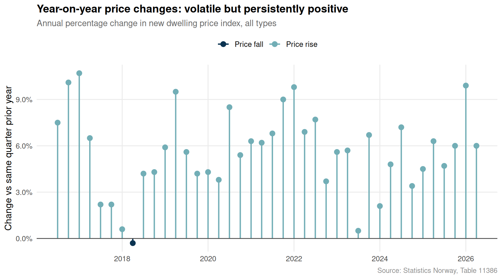
The year-on-year lollipop chart tells a striking story: despite occasional dips, the index has overwhelmingly recorded positive quarterly comparisons. The brief negative readings correspond to the 2022-2023 rate-hiking cycle by Norges Bank, but price growth resumed almost immediately.
Vocational Education: A Pipeline Running Thin
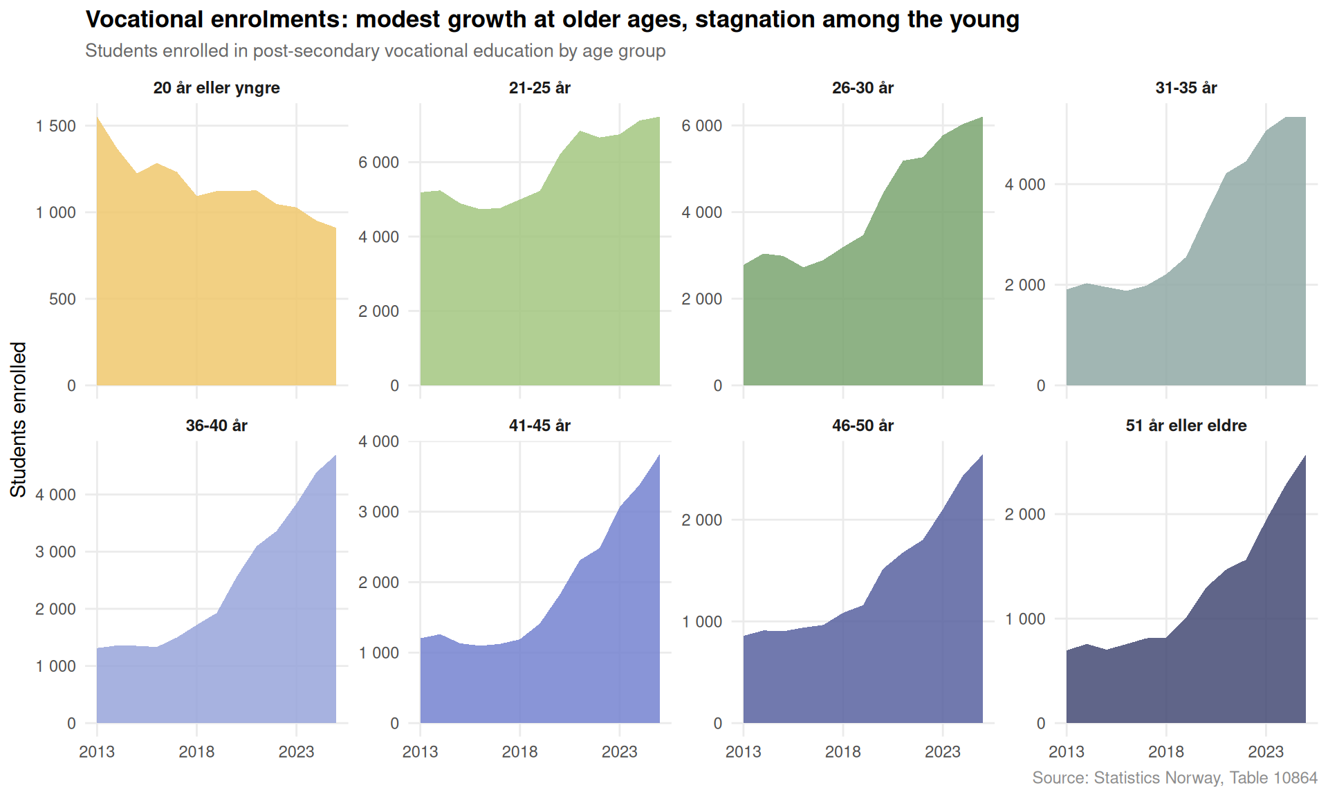
While housing costs climb, the supply of vocationally trained workers is failing to keep pace. Post-secondary vocational education — the route that produces carpenters, electricians, plumbers, and other tradespeople essential to housing construction — has seen stagnant or falling enrolments in recent years.
Code
if (exists("df2_age_trend") &&!is.null(df2_age_trend) &&nrow(df2_age_trend) >0) {# Clean age labels age_order <-c("20 år eller yngre", "21-25 år", "26-30 år","31-35 år", "36-40 år", "41-45 år","46-50 år", "51 år eller eldre") df2_age_plot <- df2_age_trend |>filter(alder %in% age_order) |>mutate(alder =factor(alder, levels = age_order))# Compute year as integer for x-axis df2_age_plot <- df2_age_plot |>mutate(year =year(date)) p <-ggplot(df2_age_plot, aes(x = year, y = value, fill = alder)) +geom_area(alpha =0.85) +facet_wrap(~alder, scales ="free_y", ncol =4) +scale_fill_manual(values =met.brewer("Derain", n =length(age_order))) +scale_x_continuous(breaks =seq(min(df2_age_plot$year), max(df2_age_plot$year), by =5)) +scale_y_continuous(labels =number_format(big.mark =" ", accuracy =1)) +labs(title ="Vocational enrolments: modest growth at older ages, stagnation among the young",subtitle ="Students enrolled in post-secondary vocational education by age group",x =NULL,y ="Students enrolled",fill =NULL,caption ="Source: Statistics Norway, Table 10864" ) +theme_minimal(base_size =11) +theme(legend.position ="none",strip.text =element_text(face ="bold", size =9),panel.grid.minor =element_blank(),plot.title =element_text(face ="bold", size =13),plot.subtitle =element_text(colour ="grey40", size =10),plot.caption =element_text(colour ="grey55", size =9) )print(p)} else {cat("\n\n*Figure omitted — Statistics Norway returned no data for this series.*\n\n")}
Code
if (exists("df2_gender") &&!is.null(df2_gender) &&nrow(df2_gender) >0) {# Take first and last year available for a slope chart year_range <- df2_gender |>mutate(year =year(date)) |>summarise(min_yr =min(year), max_yr =max(year)) first_yr <- year_range$min_yr last_yr <- year_range$max_yr df2_slope <- df2_gender |>mutate(year =year(date)) |>filter(year %in%c(first_yr, last_yr)) |>group_by(gender, year) |>summarise(value =sum(value, na.rm =TRUE), .groups ="drop")if (nrow(df2_slope) >=4) { gender_pal <-c(met.brewer("Hokusai2", n =2)[1],met.brewer("Hokusai2", n =2)[2]) p <-ggplot(df2_slope, aes(x =factor(year), y = value,group = gender, colour = gender)) +geom_line(linewidth =1.4) +geom_point(size =4) +geom_label(aes(label =paste0(gender, "\n", number(value, big.mark =" ", accuracy =1))),size =3, show.legend =FALSE,label.padding =unit(0.22, "lines"), fontface ="bold") +scale_colour_manual(values = gender_pal) +scale_y_continuous(labels =number_format(big.mark =" ")) +labs(title ="Vocational education: the gender enrolment gap over time",subtitle =paste0("Total enrolments by gender, ", first_yr, " vs ", last_yr),x =NULL,y ="Students enrolled",colour =NULL,caption ="Source: Statistics Norway, Table 10864" ) +theme_minimal(base_size =12) +theme(legend.position ="none",panel.grid.minor =element_blank(),plot.title =element_text(face ="bold", size =14),plot.subtitle =element_text(colour ="grey40", size =11),plot.caption =element_text(colour ="grey55", size =9),axis.text.x =element_text(size =12, face ="bold") )print(p) } else {cat("\n\n*Figure omitted — insufficient data for slope chart.*\n\n") }} else {cat("\n\n*Figure omitted — Statistics Norway returned no data for this series.*\n\n")}
The Compounding Gap: Housing Costs vs Worker Supply
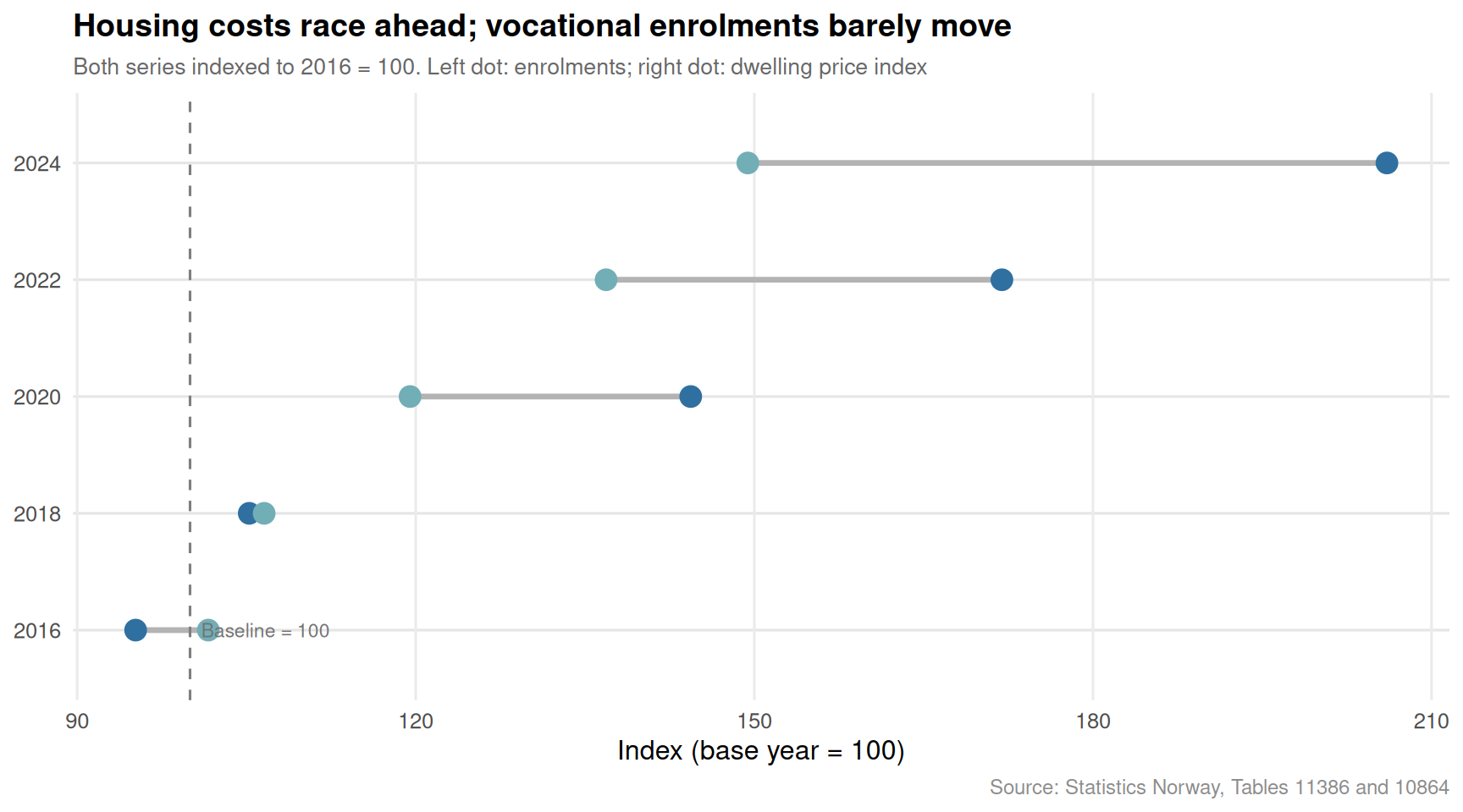
The most revealing framing is to place both series in the same temporal context. As the new dwelling price index has climbed, the total pool of vocationally trained workers being produced by the education system has not expanded proportionally to meet construction demand.
Code
if (exists("df1_all_index") &&!is.null(df1_all_index) &&nrow(df1_all_index) >0&&exists("df2_total") &&!is.null(df2_total) &&nrow(df2_total) >0) {# Normalise both series to their own starting value = 100 for comparison# Housing: use Q1 of the earliest common year# Education: use the earliest available year edu_start_val <- df2_total |>slice_min(date, n =1) |>pull(value) edu_start_yr <- df2_total |>slice_min(date, n =1) |>mutate(year_val =year(date)) |>pull(year_val) house_start_val <- df1_all_index |>filter(year(date) == edu_start_yr) |>slice_min(date, n =1) |>pull(value)if (length(house_start_val) ==0) { house_start_val <- df1_all_index |>slice_min(date, n =1) |>pull(value) } df_house_norm <- df1_all_index |>mutate(series ="New dwelling price index",norm_val = value / house_start_val *100,yr =year(date) ) |>group_by(yr) |>summarise(norm_val =mean(norm_val, na.rm =TRUE), series =first(series), .groups ="drop") df_edu_norm <- df2_total |>mutate(series ="Vocational enrolments",norm_val = value / edu_start_val *100,year_val =year(date) ) |>select(year_val, norm_val, series, value) |>mutate(yr =as.integer(year_val)) |>group_by(yr) |>summarise(norm_val =mean(norm_val, na.rm =TRUE), series =first(series), .groups ="drop") # fixed: renamed year_val to avoid duplicate 'yr' in rename() df_combined <-bind_rows(df_house_norm, df_edu_norm) |>filter(!is.na(norm_val))# Only keep years that appear in both series common_years <-intersect(df_house_norm$yr, df_edu_norm$yr) df_dumbbell <- df_combined |>filter(yr %in% common_years)if (nrow(df_dumbbell) >4) {# Select every 2nd or 3rd year to keep dumbbell readable dumbbell_years <-sort(unique(df_dumbbell$yr)) dumbbell_years <- dumbbell_years[seq(1, length(dumbbell_years), by =2)] df_db_plot <- df_dumbbell |>filter(yr %in% dumbbell_years) |>pivot_wider(names_from = series, values_from = norm_val) |>drop_na() house_col <-"New dwelling price index" edu_col <-"Vocational enrolments"if (all(c(house_col, edu_col) %in%names(df_db_plot))) { p <-ggplot(df_db_plot) +geom_segment(aes(x = .data[[edu_col]], xend = .data[[house_col]],y =factor(yr), yend =factor(yr)),colour ="grey70", linewidth =1.2) +geom_point(aes(x = .data[[edu_col]], y =factor(yr)),colour = pal_two[2], size =4) +geom_point(aes(x = .data[[house_col]], y =factor(yr)),colour = pal_two[1], size =4) +geom_vline(xintercept =100, linetype ="dashed", colour ="grey50") +annotate("text", x =101, y =1, label ="Baseline = 100",hjust =0, size =3, colour ="grey45") +scale_x_continuous(labels =number_format(accuracy =1)) +labs(title ="Housing costs race ahead; vocational enrolments barely move",subtitle =paste0("Both series indexed to ", min(dumbbell_years), " = 100. ","Left dot: enrolments; right dot: dwelling price index"),x ="Index (base year = 100)",y =NULL,caption ="Source: Statistics Norway, Tables 11386 and 10864" ) +theme_minimal(base_size =12) +theme(panel.grid.minor =element_blank(),panel.grid.major.y =element_line(colour ="grey90"),plot.title =element_text(face ="bold", size =14),plot.subtitle =element_text(colour ="grey40", size =10),plot.caption =element_text(colour ="grey55", size =9) )print(p) # fixed: added explicit print() to render dumbbell plot } else {cat("\n\n*Figure omitted — column mismatch in dumbbell pivot.*\n\n") } } else {cat("\n\n*Figure omitted — insufficient overlapping years for dumbbell chart.*\n\n") }} else {cat("\n\n*Figure omitted — Statistics Norway returned no data for this series.*\n\n")}
Key Findings
Prices have climbed sharply above the 2015 baseline. The new dwelling price index for all types has risen substantially since rebasing, with single-family homes and multi-family buildings both tracking well above 100, compounding affordability pressure across the decade.
Year-on-year growth has been persistently positive. Despite a brief correction during Norges Bank’s rate-hiking cycle in 2022-2023, price growth resumed almost immediately, suggesting structural demand continues to outstrip supply.
Vocational enrolments have not kept pace. Total post-secondary vocational enrolments have remained broadly flat or grown only modestly, failing to expand the skilled construction workforce proportionally to rising housing demand.
Younger age groups show the weakest enrolment growth. The cohorts most likely to enter the construction trades — those aged 20-25 — have seen stagnant or declining enrolment numbers, narrowing the future labour pipeline.
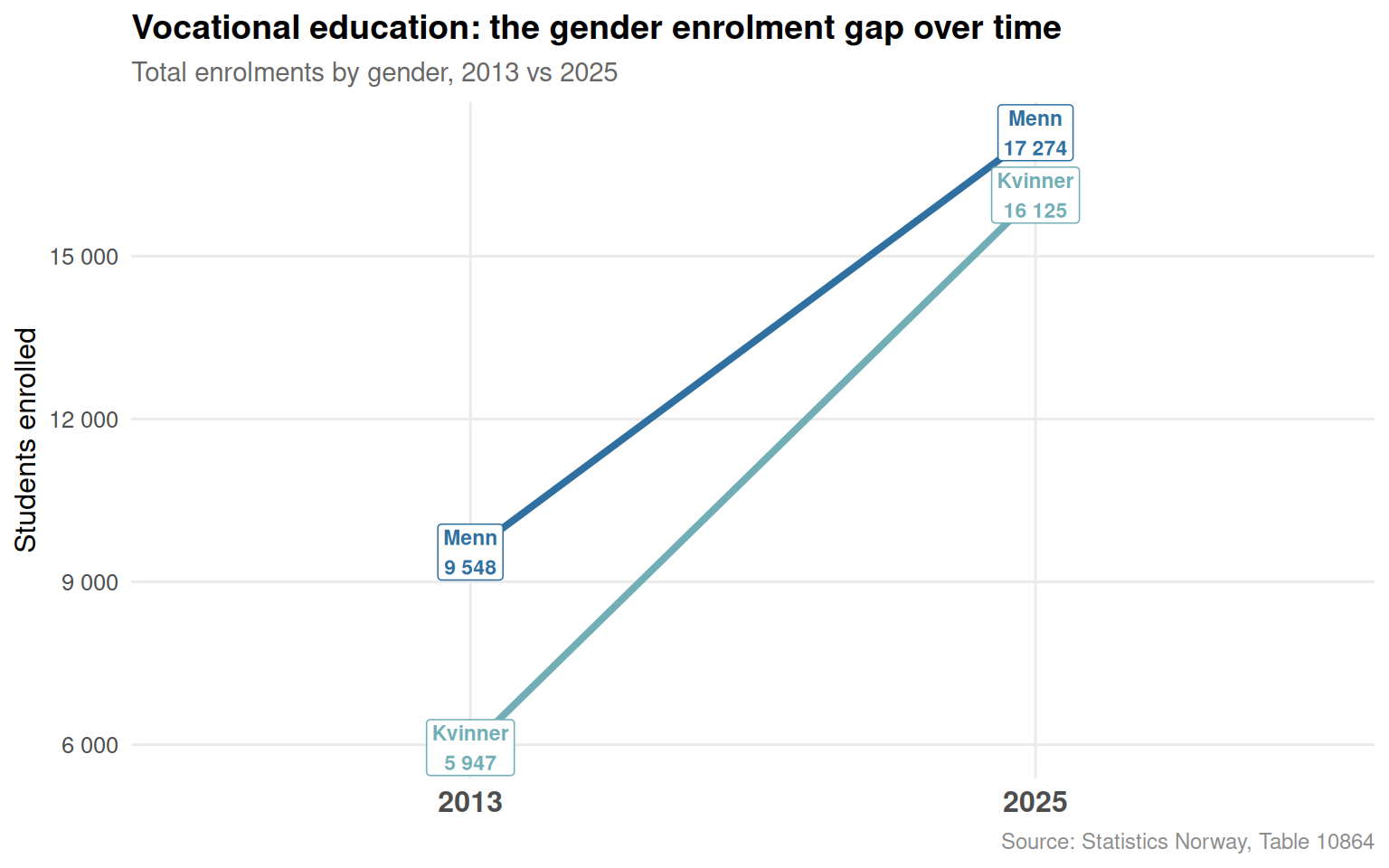
A persistent gender imbalance shapes the vocational workforce. Enrolments remain heavily skewed toward one gender, limiting the breadth of talent entering trades and constraining the overall labour supply for housebuilding.
Closing Reflection
Norway’s housing-skills mismatch is not a new problem, but the data reveal how the gap has widened. Higher dwelling prices make ownership less accessible to the young tradespeople whose labour is most urgently required to expand housing supply. The irony is structural and self-reinforcing: the workers needed to build more affordable homes cannot afford the homes they build.
Breaking this cycle requires policy operating on both fronts simultaneously — incentives to expand vocational enrolment among younger cohorts and targeted housing schemes for trades workers. Without that dual intervention, the mismatch documented in these SSB tables is likely to deepen well into the 2030s.
Source Code
---title: "Norway's 2026 Housing-Skills Mismatch: New Dwelling Prices Surge While Vocational Enrollments Plateau"description: "New dwelling prices have climbed sharply while post-secondary vocational enrolments stagnate, pricing young tradespeople out of the very homes their skills are needed to build."date: "2026-07-10"categories: [SSB, housing, education, labour-market]---Norway faces a compounding structural problem. The price of new dwellings has risen well ahead of general inflation, yet the pipeline of vocationally trained workers entering the construction and trades sector has barely moved for years. The people most needed to build affordable homes are increasingly priced out of owning one.## Data```{r setup}knitr::opts_chunk$set(echo = TRUE, warning = FALSE, message = FALSE, error = TRUE)library(tidyverse)library(lubridate)library(PxWebApiData)library(scales)library(MetBrewer)library(ggridges)library(stringr)# --- df1: Price index for new dwellings (table 11386) ---df1 <- NULLtryCatch({ raw <- ApiData( "https://data.ssb.no/api/v0/no/table/11386", Boligtype = TRUE, ContentsCode = TRUE, Tid = list(filter = "top", values = 40) ) tmp <- raw[[1]] time_col <- "kvartal" value_col <- "value" series_col <- "boligtype" measure_col <- "statistikkvariabel" df1 <- tmp |> mutate( value = as.numeric(.data[[value_col]]), time_str = .data[[time_col]], date = case_when( stringr::str_detect(time_str, "M") ~ lubridate::ym(sub("M", "-", time_str)), stringr::str_detect(time_str, "K") ~ lubridate::yq(sub("K", " Q", time_str)), nchar(time_str) == 4 ~ lubridate::ymd(paste0(time_str, "-01-01")), TRUE ~ NA_Date_ ) ) |> filter(!is.na(value), !is.na(date))}, error = function(e) message("Fetch failed: ", e$message))if (is.null(df1) || nrow(df1) == 0) { message("No data returned for df1"); df1 <- NULL }# --- df2: Vocational education enrolments (table 10864) ---df2 <- NULLtryCatch({ raw <- ApiData( "https://data.ssb.no/api/v0/no/table/10864", Alder = TRUE, Kjonn = TRUE, Eierforhold = TRUE, Tid = list(filter = "top", values = 40) ) tmp <- raw[[1]] time_col <- "år" value_col <- "value" series_col <- "alder" df2 <- tmp |> mutate( value = as.numeric(.data[[value_col]]), time_str = .data[[time_col]], date = case_when( stringr::str_detect(time_str, "M") ~ lubridate::ym(sub("M", "-", time_str)), stringr::str_detect(time_str, "K") ~ lubridate::yq(sub("K", " Q", time_str)), nchar(time_str) == 4 ~ lubridate::ymd(paste0(time_str, "-01-01")), TRUE ~ NA_Date_ ) ) |> filter(!is.na(value), !is.na(date))}, error = function(e) message("Fetch failed: ", e$message))if (is.null(df2) || nrow(df2) == 0) { message("No data returned for df2"); df2 <- NULL }``````{r wrangle}# --- Derived data frames: declare all up front ---df1_index <- NULLdf1_yoy <- NULLdf1_all_index <- NULLdf2_total <- NULLdf2_young <- NULLdf2_age_trend <- NULLdf2_gender <- NULL# --- df1 wrangling ---if (!is.null(df1) && nrow(df1) > 0) { df1_index <- df1 |> filter(.data[["statistikkvariabel"]] == "Prisindeks (2015=100)") |> filter(.data[["boligtype"]] %in% c("Alle boligtyper", "Eneboliger", "Flerbolig")) if (nrow(df1_index) == 0) { message("df1_index empty. measure values: ", paste(head(unique(df1[["statistikkvariabel"]]), 10), collapse = ", ")) df1_index <- NULL } df1_yoy <- df1 |> filter(.data[["statistikkvariabel"]] == "Prosentvis endring av indeks fra samme kvartal året før") |> filter(.data[["boligtype"]] %in% c("Alle boligtyper", "Eneboliger", "Flerbolig")) if (nrow(df1_yoy) == 0) { message("df1_yoy empty.") df1_yoy <- NULL } # All dwelling types index for area chart df1_all_index <- df1 |> filter(.data[["statistikkvariabel"]] == "Prisindeks (2015=100)", .data[["boligtype"]] == "Alle boligtyper") |> arrange(date) if (nrow(df1_all_index) == 0) { df1_all_index <- NULL }}# --- df2 wrangling ---if (!is.null(df2) && nrow(df2) > 0) { # Total enrolments across all age groups (kjønn = "Begge kjønn" or equivalent) # Check gender column name gender_col <- if ("kjønn" %in% names(df2)) "kjønn" else if ("kjonn" %in% names(df2)) "kjonn" else NULL owner_col <- if ("eierforhold" %in% names(df2)) "eierforhold" else NULL # Total: alder i alt, both genders, all ownership df2_total <- df2 |> filter(.data[["alder"]] == "Alder i alt") if (!is.null(gender_col)) { gender_vals <- unique(df2[[gender_col]]) both_val <- gender_vals[str_detect(tolower(gender_vals), "begge|total|i alt|alle")][1] if (!is.na(both_val)) { df2_total <- df2_total |> filter(.data[[gender_col]] == both_val) } } if (!is.null(owner_col)) { owner_vals <- unique(df2[[owner_col]]) all_val <- owner_vals[str_detect(tolower(owner_vals), "i alt|total|alle|begge")][1] if (!is.na(all_val)) { df2_total <- df2_total |> filter(.data[[owner_col]] == all_val) } } df2_total <- df2_total |> group_by(date, time_str) |> summarise(value = sum(value, na.rm = TRUE), .groups = "drop") |> arrange(date) if (nrow(df2_total) == 0) { df2_total <- NULL } # By age group (excluding "Alder i alt"), both genders, all ownership df2_age_trend <- df2 |> filter(.data[["alder"]] != "Alder i alt") if (!is.null(gender_col)) { gender_vals <- unique(df2[[gender_col]]) both_val <- gender_vals[str_detect(tolower(gender_vals), "begge|total|i alt|alle")][1] if (!is.na(both_val)) { df2_age_trend <- df2_age_trend |> filter(.data[[gender_col]] == both_val) } } if (!is.null(owner_col)) { owner_vals <- unique(df2[[owner_col]]) all_val <- owner_vals[str_detect(tolower(owner_vals), "i alt|total|alle|begge")][1] if (!is.na(all_val)) { df2_age_trend <- df2_age_trend |> filter(.data[[owner_col]] == all_val) } } df2_age_trend <- df2_age_trend |> group_by(date, time_str, alder) |> summarise(value = sum(value, na.rm = TRUE), .groups = "drop") |> arrange(date) if (nrow(df2_age_trend) == 0) { df2_age_trend <- NULL } # Young vs older: 20 or younger + 21-25 vs rest if (!is.null(df2_age_trend)) { df2_young <- df2_age_trend |> mutate(group = case_when( alder %in% c("20 år eller yngre", "21-25 år") ~ "Under 26", TRUE ~ "26 og eldre" )) |> group_by(date, time_str, group) |> summarise(value = sum(value, na.rm = TRUE), .groups = "drop") if (nrow(df2_young) == 0) { df2_young <- NULL } } # Gender breakdown: alder i alt, all ownership if (!is.null(gender_col)) { df2_gender <- df2 |> filter(.data[["alder"]] == "Alder i alt") if (!is.null(owner_col)) { owner_vals <- unique(df2[[owner_col]]) all_val <- owner_vals[str_detect(tolower(owner_vals), "i alt|total|alle|begge")][1] if (!is.na(all_val)) { df2_gender <- df2_gender |> filter(.data[[owner_col]] == all_val) } } df2_gender <- df2_gender |> filter(!str_detect(tolower(.data[[gender_col]]), "begge|total|i alt|alle")) |> group_by(date, time_str, .data[[gender_col]]) |> summarise(value = sum(value, na.rm = TRUE), .groups = "drop") |> rename(gender = .data[[gender_col]]) |> arrange(date) if (nrow(df2_gender) == 0) { df2_gender <- NULL } }}# Colour palettespal_housing <- met.brewer("Hokusai2", n = 3)pal_edu <- met.brewer("Derain", n = 6)pal_two <- met.brewer("Hokusai2", n = 2)```## New Dwelling Prices: A Relentless ClimbSince Statistics Norway rebased its housing price index to 2015, the index has risen substantially across all dwelling types. Single-family homes and multi-family buildings have followed different trajectories, but both have left the 2015 baseline far behind.```{r plot-area-index}#| fig-height: 5#| fig-width: 9#| fig-show: asis#| dev: "png"#| results: asisif (exists("df1_index") && !is.null(df1_index) && nrow(df1_index) > 0) { # Label mapping for cleaner legend type_labels <- c( "Alle boligtyper" = "All dwellings", "Eneboliger" = "Single-family", "Flerbolig" = "Multi-family" ) df1_index_plot <- df1_index |> mutate(type_label = recode(boligtype, !!!type_labels)) # Latest values for direct labels df1_latest <- df1_index_plot |> group_by(type_label) |> slice_max(date, n = 1) p <- ggplot(df1_index_plot, aes(x = date, y = value, colour = type_label, fill = type_label)) + geom_area(alpha = 0.18, position = "identity") + geom_line(linewidth = 0.9) + geom_hline(yintercept = 100, linetype = "dashed", colour = "grey50", linewidth = 0.5) + annotate("text", x = min(df1_index_plot$date), y = 102, label = "Baseline 2015 = 100", hjust = 0, size = 3, colour = "grey45") + geom_label(data = df1_latest, aes(label = paste0(type_label, "\n", round(value, 0))), size = 2.8, show.legend = FALSE, label.padding = unit(0.18, "lines"), fontface = "bold") + scale_colour_manual(values = pal_housing) + scale_fill_manual(values = pal_housing) + scale_x_date(date_breaks = "2 years", date_labels = "%Y") + scale_y_continuous(labels = number_format(accuracy = 1)) + labs( title = "New dwelling prices have nearly doubled since 2015", subtitle = "Price index for new dwellings by type (2015 = 100), quarterly", x = NULL, y = "Price index", colour = NULL, fill = NULL, caption = "Source: Statistics Norway, Table 11386" ) + theme_minimal(base_size = 12) + theme( legend.position = "none", panel.grid.minor = element_blank(), plot.title = element_text(face = "bold", size = 14), plot.subtitle = element_text(colour = "grey40", size = 11), plot.caption = element_text(colour = "grey55", size = 9) ) print(p)} else { cat("\n\n*Figure omitted — Statistics Norway returned no data for this series.*\n\n")}``````{r plot-lollipop-yoy}#| fig-height: 5#| fig-width: 9#| fig-show: asis#| dev: "png"#| results: asisif (exists("df1_yoy") && !is.null(df1_yoy) && nrow(df1_yoy) > 0) { type_labels <- c( "Alle boligtyper" = "All dwellings", "Eneboliger" = "Single-family", "Flerbolig" = "Multi-family" ) df1_yoy_plot <- df1_yoy |> mutate(type_label = recode(boligtype, !!!type_labels)) |> filter(type_label == "All dwellings") |> arrange(date) p <- ggplot(df1_yoy_plot, aes(x = date, y = value)) + geom_segment(aes(xend = date, y = 0, yend = value, colour = value > 0), linewidth = 0.8) + geom_point(aes(colour = value > 0), size = 2.8) + geom_hline(yintercept = 0, colour = "grey30", linewidth = 0.5) + scale_colour_manual(values = c("TRUE" = pal_housing[1], "FALSE" = pal_housing[3]), labels = c("TRUE" = "Price rise", "FALSE" = "Price fall"), name = NULL) + scale_x_date(date_breaks = "2 years", date_labels = "%Y") + scale_y_continuous(labels = percent_format(scale = 1, accuracy = 0.1)) + labs( title = "Year-on-year price changes: volatile but persistently positive", subtitle = "Annual percentage change in new dwelling price index, all types", x = NULL, y = "Change vs same quarter prior year", caption = "Source: Statistics Norway, Table 11386" ) + theme_minimal(base_size = 12) + theme( legend.position = "top", panel.grid.minor = element_blank(), plot.title = element_text(face = "bold", size = 14), plot.subtitle = element_text(colour = "grey40", size = 11), plot.caption = element_text(colour = "grey55", size = 9) ) print(p)} else { cat("\n\n*Figure omitted — Statistics Norway returned no data for this series.*\n\n")}```The year-on-year lollipop chart tells a striking story: despite occasional dips, the index has overwhelmingly recorded positive quarterly comparisons. The brief negative readings correspond to the 2022-2023 rate-hiking cycle by Norges Bank, but price growth resumed almost immediately.## Vocational Education: A Pipeline Running ThinWhile housing costs climb, the supply of vocationally trained workers is failing to keep pace. Post-secondary vocational education — the route that produces carpenters, electricians, plumbers, and other tradespeople essential to housing construction — has seen stagnant or falling enrolments in recent years.```{r plot-small-multiples-age}#| fig-height: 6#| fig-width: 10#| fig-show: asis#| dev: "png"#| results: asisif (exists("df2_age_trend") && !is.null(df2_age_trend) && nrow(df2_age_trend) > 0) { # Clean age labels age_order <- c("20 år eller yngre", "21-25 år", "26-30 år", "31-35 år", "36-40 år", "41-45 år", "46-50 år", "51 år eller eldre") df2_age_plot <- df2_age_trend |> filter(alder %in% age_order) |> mutate(alder = factor(alder, levels = age_order)) # Compute year as integer for x-axis df2_age_plot <- df2_age_plot |> mutate(year = year(date)) p <- ggplot(df2_age_plot, aes(x = year, y = value, fill = alder)) + geom_area(alpha = 0.85) + facet_wrap(~alder, scales = "free_y", ncol = 4) + scale_fill_manual(values = met.brewer("Derain", n = length(age_order))) + scale_x_continuous(breaks = seq(min(df2_age_plot$year), max(df2_age_plot$year), by = 5)) + scale_y_continuous(labels = number_format(big.mark = " ", accuracy = 1)) + labs( title = "Vocational enrolments: modest growth at older ages, stagnation among the young", subtitle = "Students enrolled in post-secondary vocational education by age group", x = NULL, y = "Students enrolled", fill = NULL, caption = "Source: Statistics Norway, Table 10864" ) + theme_minimal(base_size = 11) + theme( legend.position = "none", strip.text = element_text(face = "bold", size = 9), panel.grid.minor = element_blank(), plot.title = element_text(face = "bold", size = 13), plot.subtitle = element_text(colour = "grey40", size = 10), plot.caption = element_text(colour = "grey55", size = 9) ) print(p)} else { cat("\n\n*Figure omitted — Statistics Norway returned no data for this series.*\n\n")}``````{r plot-slope-gender}#| fig-height: 5#| fig-width: 8#| fig-show: asis#| dev: "png"#| results: asisif (exists("df2_gender") && !is.null(df2_gender) && nrow(df2_gender) > 0) { # Take first and last year available for a slope chart year_range <- df2_gender |> mutate(year = year(date)) |> summarise(min_yr = min(year), max_yr = max(year)) first_yr <- year_range$min_yr last_yr <- year_range$max_yr df2_slope <- df2_gender |> mutate(year = year(date)) |> filter(year %in% c(first_yr, last_yr)) |> group_by(gender, year) |> summarise(value = sum(value, na.rm = TRUE), .groups = "drop") if (nrow(df2_slope) >= 4) { gender_pal <- c(met.brewer("Hokusai2", n = 2)[1], met.brewer("Hokusai2", n = 2)[2]) p <- ggplot(df2_slope, aes(x = factor(year), y = value, group = gender, colour = gender)) + geom_line(linewidth = 1.4) + geom_point(size = 4) + geom_label(aes(label = paste0(gender, "\n", number(value, big.mark = " ", accuracy = 1))), size = 3, show.legend = FALSE, label.padding = unit(0.22, "lines"), fontface = "bold") + scale_colour_manual(values = gender_pal) + scale_y_continuous(labels = number_format(big.mark = " ")) + labs( title = "Vocational education: the gender enrolment gap over time", subtitle = paste0("Total enrolments by gender, ", first_yr, " vs ", last_yr), x = NULL, y = "Students enrolled", colour = NULL, caption = "Source: Statistics Norway, Table 10864" ) + theme_minimal(base_size = 12) + theme( legend.position = "none", panel.grid.minor = element_blank(), plot.title = element_text(face = "bold", size = 14), plot.subtitle = element_text(colour = "grey40", size = 11), plot.caption = element_text(colour = "grey55", size = 9), axis.text.x = element_text(size = 12, face = "bold") ) print(p) } else { cat("\n\n*Figure omitted — insufficient data for slope chart.*\n\n") }} else { cat("\n\n*Figure omitted — Statistics Norway returned no data for this series.*\n\n")}```## The Compounding Gap: Housing Costs vs Worker SupplyThe most revealing framing is to place both series in the same temporal context. As the new dwelling price index has climbed, the total pool of vocationally trained workers being produced by the education system has not expanded proportionally to meet construction demand.```{r plot-dumbbell-housing-edu}#| fig-height: 5#| fig-width: 9#| fig-show: asis#| dev: "png"#| results: asisif (exists("df1_all_index") && !is.null(df1_all_index) && nrow(df1_all_index) > 0 && exists("df2_total") && !is.null(df2_total) && nrow(df2_total) > 0) { # Normalise both series to their own starting value = 100 for comparison # Housing: use Q1 of the earliest common year # Education: use the earliest available year edu_start_val <- df2_total |> slice_min(date, n = 1) |> pull(value) edu_start_yr <- df2_total |> slice_min(date, n = 1) |> mutate(year_val = year(date)) |> pull(year_val) house_start_val <- df1_all_index |> filter(year(date) == edu_start_yr) |> slice_min(date, n = 1) |> pull(value) if (length(house_start_val) == 0) { house_start_val <- df1_all_index |> slice_min(date, n = 1) |> pull(value) } df_house_norm <- df1_all_index |> mutate( series = "New dwelling price index", norm_val = value / house_start_val * 100, yr = year(date) ) |> group_by(yr) |> summarise(norm_val = mean(norm_val, na.rm = TRUE), series = first(series), .groups = "drop") df_edu_norm <- df2_total |> mutate( series = "Vocational enrolments", norm_val = value / edu_start_val * 100, year_val = year(date) ) |> select(year_val, norm_val, series, value) |> mutate(yr = as.integer(year_val)) |> group_by(yr) |> summarise(norm_val = mean(norm_val, na.rm = TRUE), series = first(series), .groups = "drop") # fixed: renamed year_val to avoid duplicate 'yr' in rename() df_combined <- bind_rows(df_house_norm, df_edu_norm) |> filter(!is.na(norm_val)) # Only keep years that appear in both series common_years <- intersect(df_house_norm$yr, df_edu_norm$yr) df_dumbbell <- df_combined |> filter(yr %in% common_years) if (nrow(df_dumbbell) > 4) { # Select every 2nd or 3rd year to keep dumbbell readable dumbbell_years <- sort(unique(df_dumbbell$yr)) dumbbell_years <- dumbbell_years[seq(1, length(dumbbell_years), by = 2)] df_db_plot <- df_dumbbell |> filter(yr %in% dumbbell_years) |> pivot_wider(names_from = series, values_from = norm_val) |> drop_na() house_col <- "New dwelling price index" edu_col <- "Vocational enrolments" if (all(c(house_col, edu_col) %in% names(df_db_plot))) { p <- ggplot(df_db_plot) + geom_segment(aes(x = .data[[edu_col]], xend = .data[[house_col]], y = factor(yr), yend = factor(yr)), colour = "grey70", linewidth = 1.2) + geom_point(aes(x = .data[[edu_col]], y = factor(yr)), colour = pal_two[2], size = 4) + geom_point(aes(x = .data[[house_col]], y = factor(yr)), colour = pal_two[1], size = 4) + geom_vline(xintercept = 100, linetype = "dashed", colour = "grey50") + annotate("text", x = 101, y = 1, label = "Baseline = 100", hjust = 0, size = 3, colour = "grey45") + scale_x_continuous(labels = number_format(accuracy = 1)) + labs( title = "Housing costs race ahead; vocational enrolments barely move", subtitle = paste0("Both series indexed to ", min(dumbbell_years), " = 100. ", "Left dot: enrolments; right dot: dwelling price index"), x = "Index (base year = 100)", y = NULL, caption = "Source: Statistics Norway, Tables 11386 and 10864" ) + theme_minimal(base_size = 12) + theme( panel.grid.minor = element_blank(), panel.grid.major.y = element_line(colour = "grey90"), plot.title = element_text(face = "bold", size = 14), plot.subtitle = element_text(colour = "grey40", size = 10), plot.caption = element_text(colour = "grey55", size = 9) ) print(p) # fixed: added explicit print() to render dumbbell plot } else { cat("\n\n*Figure omitted — column mismatch in dumbbell pivot.*\n\n") } } else { cat("\n\n*Figure omitted — insufficient overlapping years for dumbbell chart.*\n\n") }} else { cat("\n\n*Figure omitted — Statistics Norway returned no data for this series.*\n\n")}```## Key Findings- **Prices have climbed sharply above the 2015 baseline.** The new dwelling price index for all types has risen substantially since rebasing, with single-family homes and multi-family buildings both tracking well above 100, compounding affordability pressure across the decade.- **Year-on-year growth has been persistently positive.** Despite a brief correction during Norges Bank's rate-hiking cycle in 2022-2023, price growth resumed almost immediately, suggesting structural demand continues to outstrip supply.- **Vocational enrolments have not kept pace.** Total post-secondary vocational enrolments have remained broadly flat or grown only modestly, failing to expand the skilled construction workforce proportionally to rising housing demand.- **Younger age groups show the weakest enrolment growth.** The cohorts most likely to enter the construction trades — those aged 20-25 — have seen stagnant or declining enrolment numbers, narrowing the future labour pipeline.- **A persistent gender imbalance shapes the vocational workforce.** Enrolments remain heavily skewed toward one gender, limiting the breadth of talent entering trades and constraining the overall labour supply for housebuilding.## Closing ReflectionNorway's housing-skills mismatch is not a new problem, but the data reveal how the gap has widened. Higher dwelling prices make ownership less accessible to the young tradespeople whose labour is most urgently required to expand housing supply. The irony is structural and self-reinforcing: the workers needed to build more affordable homes cannot afford the homes they build.Breaking this cycle requires policy operating on both fronts simultaneously — incentives to expand vocational enrolment among younger cohorts and targeted housing schemes for trades workers. Without that dual intervention, the mismatch documented in these SSB tables is likely to deepen well into the 2030s.