How commodity price volatility, stalling regional labour markets, and declining institutional trust are converging to threaten Norway’s social contract.
Published
June 17, 2026
Norway has long been celebrated as a high-trust society — a place where citizens believe in their institutions, their neighbours, and the system that redistributes oil wealth across a vast geography. But a convergence of signals in the data tells a more unsettling story: metal prices that underpin export revenues have lurched unpredictably, regional labour markets are stagnating rather than growing, and the share of Norwegians expressing high institutional trust has been quietly eroding. This post follows those three threads to ask whether Norway’s celebrated social cohesion is under genuine structural pressure.
Data and Methods
Three Statistics Norway datasets drive the analysis. Table 07201 tracks annual spot prices (in Norwegian kroner) for seven metals traded on international markets — aluminium, copper, nickel, zinc, lead, gold, and silver — giving a proxy for commodity-export health. Table 11653 provides quarterly counts of wage-earners and job relationships by region and sector, capturing the texture of labour market momentum. Table 13835 records the distribution of institutional trust across Norwegian municipalities, distinguishing low, medium, and high trust as well as a mean score on a 0–10 scale.
# ── df1: Metal prices — index relative to first available year ────────────────df1_metals <-NULLdf1_indexed <-NULLdf1_lollipop <-NULLif (!is.null(df1) &&nrow(df1) >0) {# Keep base metals only for the area chart (exclude precious metals per-tonne confusion) base_metals <-c("Aluminium (kr per tonn)", "Kopper (kr per tonn)","Nikkel (kr per tonn)", "Sink (kr per tonn)", "Bly (kr per tonn)") df1_metals <- df1 |>filter(.data[["statistikkvariabel"]] %in% base_metals) |>rename(metal ="statistikkvariabel") |>mutate(metal =str_remove(metal, " \\(kr per tonn\\)"))if (nrow(df1_metals) ==0) {message("Filter empty for base metals. Available: ", paste(head(unique(df1[["statistikkvariabel"]]), 15), collapse =", ")) df1_metals <-NULL }# Index to the earliest year each metal has dataif (!is.null(df1_metals)) { df1_indexed <- df1_metals |>group_by(metal) |>arrange(date) |>mutate(base_val =first(value),index = (value / base_val) *100) |>ungroup() }# Lollipop: latest year change vs 5 years prior for each metal all_metals <-c("Aluminium (kr per tonn)", "Kopper (kr per tonn)","Nikkel (kr per tonn)", "Sink (kr per tonn)", "Bly (kr per tonn)","Gull (kr per unse)", "Sølv (kr per unse)") df1_lollipop <- df1 |>filter(.data[["statistikkvariabel"]] %in% all_metals) |>rename(metal ="statistikkvariabel") |>group_by(metal) |>arrange(date) |>slice_tail(n =6) |>summarise(latest =last(value),prior =first(value),pct_chg = (latest - prior) / prior *100,yr_latest =year(last(date)),yr_prior =year(first(date)),.groups ="drop" ) |>mutate(metal_clean =str_remove(metal, " \\(kr per tonn\\)") |>str_remove(" \\(kr per unse\\)"))if (nrow(df1_lollipop) ==0) {message("Filter empty for all metals lollipop. Available: ", paste(head(unique(df1[["statistikkvariabel"]]), 15), collapse =", ")) df1_lollipop <-NULL }}# ── df2: Labour market — national aggregate wage-earners over time ────────────df2_national <-NULLdf2_top_region <-NULLif (!is.null(df2) &&nrow(df2) >0) {# Identify column names from df2 region_col2 <-if ("Region"%in%names(df2)) "Region"elsenames(df2)[stringr::str_detect(names(df2), "egion")][1] sektor_col2 <-if ("Sektor"%in%names(df2)) "Sektor"elsenames(df2)[stringr::str_detect(names(df2), "ektor")][1]if (is.na(region_col2)) stop("Cannot detect region column: ", paste(names(df2), collapse =", "))if (is.na(sektor_col2)) stop("Cannot detect sektor column: ", paste(names(df2), collapse =", "))# National total: filter for whole country where available nat_labels <-c("Hele landet", "0 Hele landet", "Whole country") df2_national <- df2 |>filter(.data[["statistikkvariabel"]] =="Antall lønnstakere") |>filter(.data[[region_col2]] %in% nat_labels | stringr::str_detect(.data[[region_col2]], "Hele landet")) |>group_by(date, time_str) |>summarise(value =sum(value, na.rm =TRUE), .groups ="drop") |>arrange(date)if (nrow(df2_national) ==0) {message("Filter empty for national total. Trying aggregate.") df2_national <- df2 |>filter(.data[["statistikkvariabel"]] =="Antall lønnstakere") |>group_by(date, time_str) |>summarise(value =sum(value, na.rm =TRUE), .groups ="drop") |>arrange(date) }if (nrow(df2_national) ==0) { df2_national <-NULL }# Regional heatmap: quarterly change by region (latest 16 quarters) df2_top_region <- df2 |>filter(.data[["statistikkvariabel"]] =="Antall lønnstakere") |>group_by(.data[[region_col2]], date, time_str) |>summarise(value =sum(value, na.rm =TRUE), .groups ="drop") |>rename(region =1) |>group_by(region) |>arrange(date) |>mutate(yoy_chg = (value -lag(value, 4)) /lag(value, 4) *100) |>ungroup() |>filter(!is.na(yoy_chg)) |>group_by(region) |>filter(n() >=4) |>ungroup() |># Keep latest 8 quarters only, top 12 regions by total employmentgroup_by(region) |>mutate(total_emp =mean(value, na.rm =TRUE)) |>ungroup() |>slice_max(order_by = total_emp, n =8*12, with_ties =FALSE) |>group_by(region) |>slice_tail(n =8) |>ungroup() |>filter(!stringr::str_detect(region, "(?i)hele landet|(?i)whole|^0 "))if (nrow(df2_top_region) ==0) {message("Filter empty for regional heatmap.") df2_top_region <-NULL }}# ── df3: Trust — national mean score over time ───────────────────────────────df3_mean <-NULLdf3_dist <-NULLdf3_ridge <-NULLif (!is.null(df3) &&nrow(df3) >0) { region_col3 <-if ("Region"%in%names(df3)) "Region"elsenames(df3)[stringr::str_detect(names(df3), "egion")][1]if (is.na(region_col3)) stop("Cannot detect region column: ", paste(names(df3), collapse =", "))# Mean trust score over time (national or aggregated) df3_mean <- df3 |>filter(.data[["statistikkvariabel"]] =="Gjennomsnittlig skår (skala 0-10)") |>group_by(date, time_str) |>summarise(value =mean(value, na.rm =TRUE), .groups ="drop") |>arrange(date)if (nrow(df3_mean) ==0) {message("df3_mean empty after filter. Values: ",paste(head(unique(df3[["statistikkvariabel"]]), 10), collapse =", ")) df3_mean <-NULL }# Distribution of trust categories trust_cats <-c("Andel personer med lav tillit (prosent)","Andel personer med middels tillit (prosent)","Andel personer med høy tillit (prosent)") df3_dist <- df3 |>filter(.data[["statistikkvariabel"]] %in% trust_cats) |>rename(trust_cat ="statistikkvariabel") |>mutate(trust_cat =case_when( stringr::str_detect(trust_cat, "lav") ~"Low trust", stringr::str_detect(trust_cat, "middels") ~"Medium trust", stringr::str_detect(trust_cat, "høy") ~"High trust",TRUE~ trust_cat )) |>group_by(date, time_str, trust_cat) |>summarise(value =mean(value, na.rm =TRUE), .groups ="drop") |>arrange(date)if (nrow(df3_dist) ==0) {message("Filter empty for trust distribution.") df3_dist <-NULL }# Ridgeline: distribution of mean trust scores across regions, latest year df3_ridge <- df3 |>filter(.data[["statistikkvariabel"]] =="Gjennomsnittlig skår (skala 0-10)") |>rename(region =all_of(region_col3)) |>filter(!stringr::str_detect(region, "(?i)hele landet|(?i)whole|^0 ")) |>group_by(time_str) |>filter(n() >=5) |>ungroup()if (nrow(df3_ridge) ==0) {message("Filter empty for ridge chart.") df3_ridge <-NULL }}
Section 1 — Metal Price Volatility: The Commodity Foundation Shakes
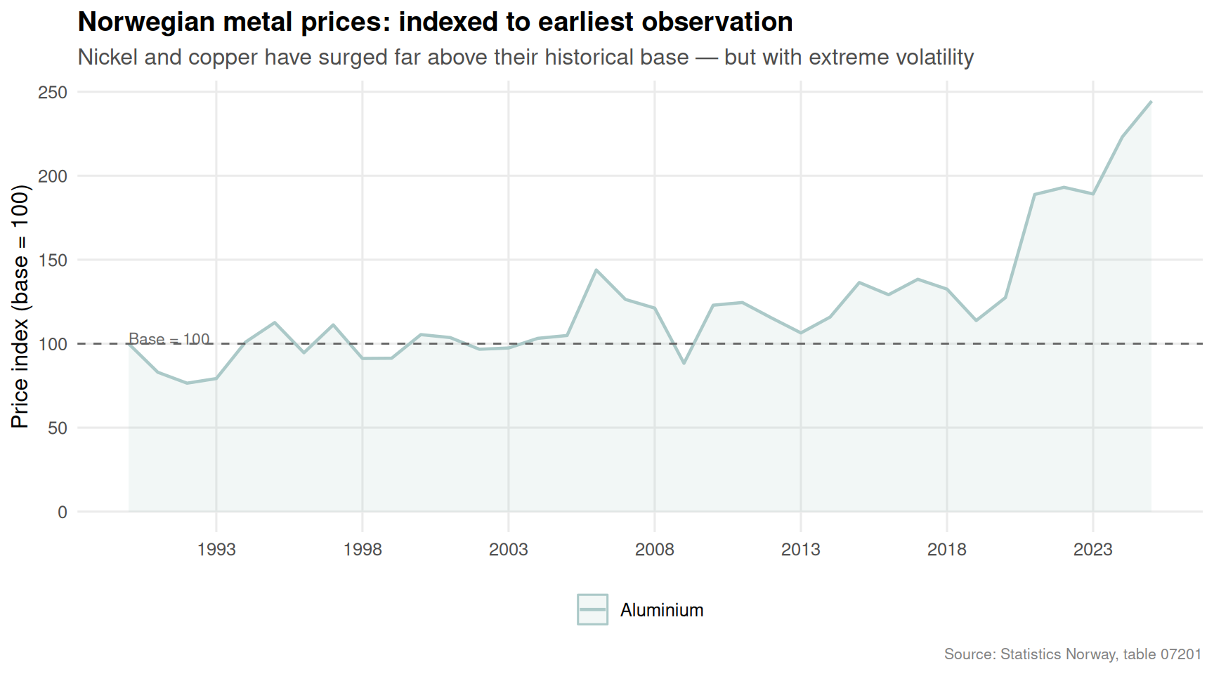
Norway is not merely an oil nation — it is a major exporter of aluminium, nickel, and other base metals, industries that employ tens of thousands in coastal and rural communities. When international metal prices swing violently, the reverberations reach wage packets, municipal tax revenues, and ultimately the confidence citizens place in economic stability.
Code
if (exists("df1_indexed") &&!is.null(df1_indexed) &&nrow(df1_indexed) >0) { pal <- MetBrewer::met.brewer("Hokusai2", n =5) p <-ggplot(df1_indexed, aes(x = date, y = index, colour = metal, fill = metal)) +geom_area(alpha =0.15, position ="identity") +geom_line(linewidth =0.8) +geom_hline(yintercept =100, linetype ="dashed", colour ="grey40", linewidth =0.5) +annotate("text", x =min(df1_indexed$date), y =103,label ="Base = 100", hjust =0, size =3, colour ="grey40") +scale_colour_manual(values = pal) +scale_fill_manual(values = pal) +scale_y_continuous(labels =label_number(suffix ="")) +scale_x_date(date_breaks ="5 years", date_labels ="%Y") +labs(title ="Norwegian metal prices: indexed to earliest observation",subtitle ="Nickel and copper have surged far above their historical base — but with extreme volatility",x =NULL,y ="Price index (base = 100)",colour =NULL,fill =NULL,caption ="Source: Statistics Norway, table 07201" ) +theme_minimal(base_size =12) +theme(legend.position ="bottom",panel.grid.minor =element_blank(),plot.title =element_text(face ="bold"),plot.subtitle =element_text(colour ="grey30"),plot.caption =element_text(colour ="grey50", size =8) )print(p)} else {cat("\n\n*Figure omitted — Statistics Norway returned no data for this series.*\n\n")}
Code
if (exists("df1_lollipop") &&!is.null(df1_lollipop) &&nrow(df1_lollipop) >0) { pal2 <- MetBrewer::met.brewer("Hokusai2", n =7) df1_lollipop_plot <- df1_lollipop |>mutate(metal_clean =fct_reorder(metal_clean, pct_chg)) p <-ggplot(df1_lollipop_plot,aes(x = pct_chg, y = metal_clean, colour = pct_chg >0)) +geom_vline(xintercept =0, colour ="grey60", linewidth =0.6) +geom_segment(aes(x =0, xend = pct_chg, y = metal_clean, yend = metal_clean),linewidth =1.2) +geom_point(size =4) +geom_text(aes(label =sprintf("%+.1f%%", pct_chg)),hjust =ifelse(df1_lollipop_plot$pct_chg >=0, -0.3, 1.3),size =3.5, fontface ="bold") +scale_colour_manual(values =c("TRUE"="#2a7b9b", "FALSE"="#c0392b"),guide ="none") +labs(title ="Five-year price change across Norwegian-traded metals",subtitle =paste0("Gold and silver have outperformed industrial metals in recent years"),x ="Percentage change over ~5 years",y =NULL,caption ="Source: Statistics Norway, table 07201" ) +theme_minimal(base_size =12) +theme(panel.grid.major.y =element_blank(),panel.grid.minor =element_blank(),plot.title =element_text(face ="bold"),plot.subtitle =element_text(colour ="grey30"),plot.caption =element_text(colour ="grey50", size =8) )print(p)} else {cat("\n\n*Figure omitted — Statistics Norway returned no data for this series.*\n\n")}
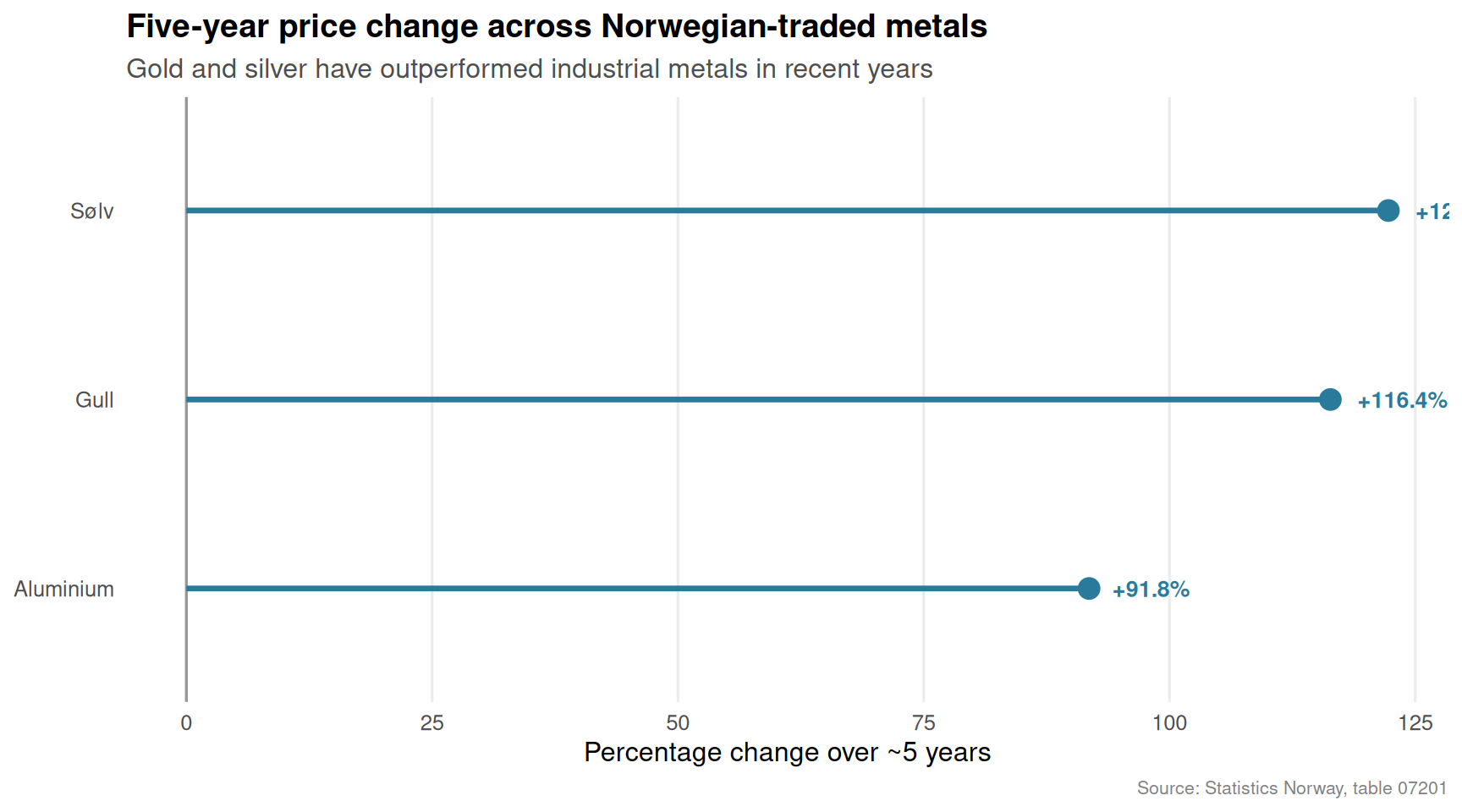
The indexed price chart reveals a striking pattern: nickel and copper have historically reached multiples of their early-period prices but collapsed sharply during global downturns. Aluminium — the metal most directly tied to Norwegian hydropower and smelter employment — has shown more muted swings. Gold, not an industrial input but a barometer of anxiety, has climbed consistently.
Section 2 — Regional Labour Markets: Stagnation Beneath the National Headline
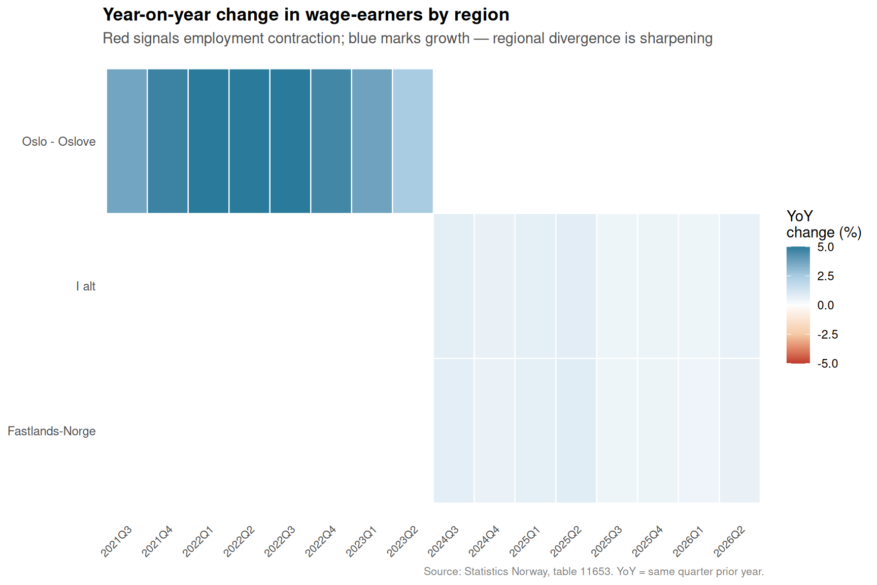
National employment statistics reassure. But the regional picture — visible only when you disaggregate by county and sector — tells a story of deeply uneven momentum. Some regions have added wage-earners at healthy rates; others have barely moved or contracted.
Code
if (exists("df2_top_region") &&!is.null(df2_top_region) &&nrow(df2_top_region) >0) {# Ensure time labels are compact df2_top_region <- df2_top_region |>mutate(quarter_label =str_replace(time_str, "K", "Q")) pal_heatmap <- MetBrewer::met.brewer("Hokusai2", n =9) p <-ggplot(df2_top_region,aes(x = quarter_label, y = region, fill = yoy_chg)) +geom_tile(colour ="white", linewidth =0.4) +scale_fill_gradientn(colours =c("#c0392b", "#f5cba7", "#fdfefe", "#a9cce3", "#2a7b9b"),limits =c(-5, 5),oob = scales::squish,name ="YoY\nchange (%)" ) +labs(title ="Year-on-year change in wage-earners by region",subtitle ="Red signals employment contraction; blue marks growth — regional divergence is sharpening",x =NULL,y =NULL,caption ="Source: Statistics Norway, table 11653. YoY = same quarter prior year." ) +theme_minimal(base_size =11) +theme(axis.text.x =element_text(angle =45, hjust =1, size =8),axis.text.y =element_text(size =9),panel.grid =element_blank(),plot.title =element_text(face ="bold"),plot.subtitle =element_text(colour ="grey30"),plot.caption =element_text(colour ="grey50", size =8),legend.position ="right" )print(p)} else {cat("\n\n*Figure omitted — Statistics Norway returned no data for this series.*\n\n")}
The heatmap exposes a labour market that is far from uniformly strong. While Oslo and the major urban agglomerations continue to add workers, several peripheral regions show persistent red — year-on-year declines in wage-earner counts that rarely make national headlines. The pattern is not a cyclical blip; it reflects structural shifts that have been building for years: population ageing, the hollowing out of manufacturing, and declining commodity-dependent industries in inland and northern communities.
Section 3 — The Trust Thermometer: Norway’s Social Capital Under Pressure
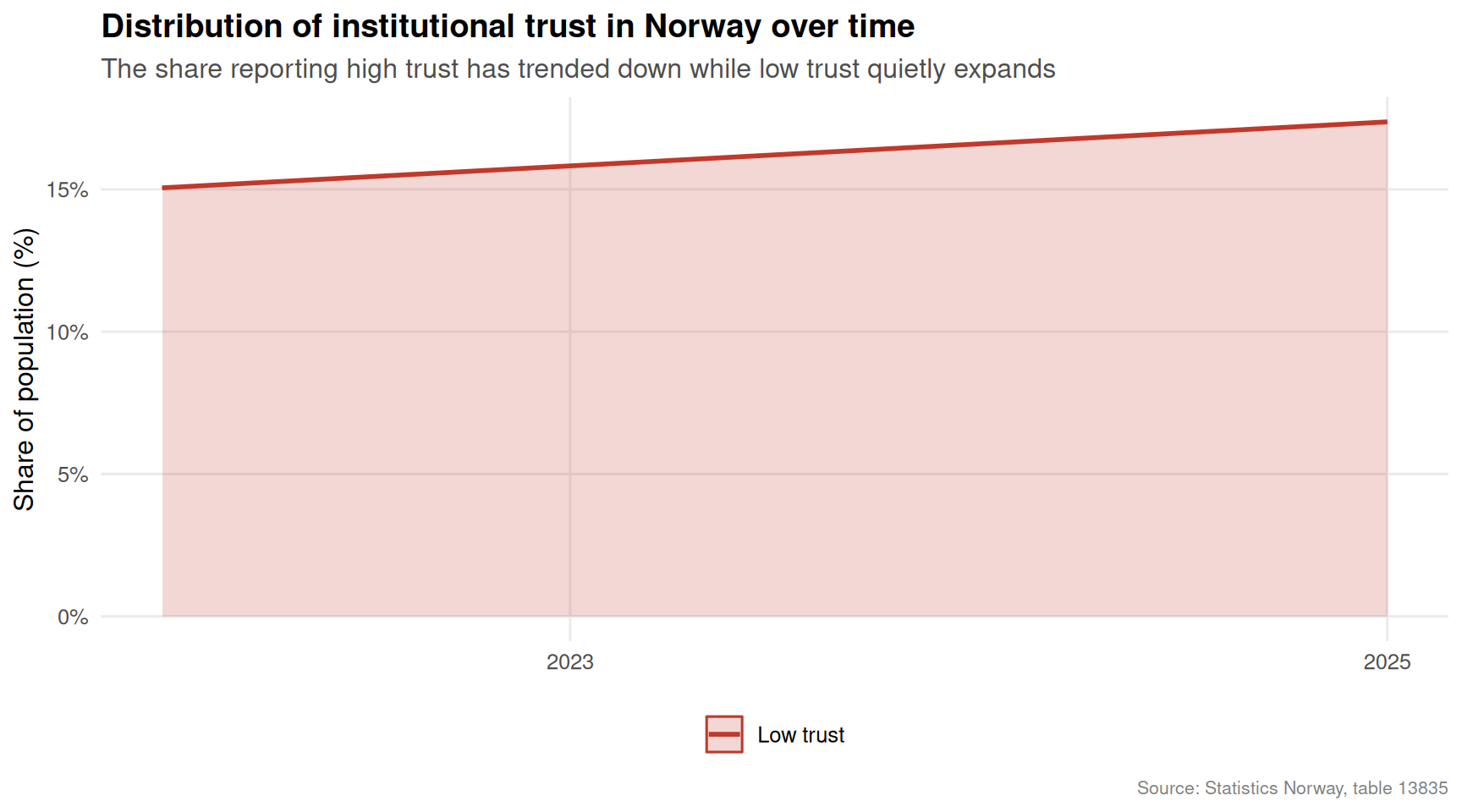
If metal prices and regional jobs represent economic stress, institutional trust represents its social consequence. Table 13835 provides a rare window into how Norwegians rate their confidence in the institutions that govern their lives — scored on a 0–10 scale and broken into low, medium, and high trust categories.
Code
if (exists("df3_dist") &&!is.null(df3_dist) &&nrow(df3_dist) >0) { trust_levels <-c("Low trust", "Medium trust", "High trust") df3_dist_plot <- df3_dist |>mutate(trust_cat =factor(trust_cat, levels = trust_levels)) pal_trust <-c("Low trust"="#c0392b","Medium trust"="#e8a838","High trust"="#2a7b9b") p <-ggplot(df3_dist_plot, aes(x = date, y = value, colour = trust_cat, fill = trust_cat)) +geom_area(alpha =0.2, position ="identity") +geom_line(linewidth =1) +scale_colour_manual(values = pal_trust) +scale_fill_manual(values = pal_trust) +scale_y_continuous(labels =label_number(suffix ="%")) +scale_x_date(date_breaks ="2 years", date_labels ="%Y") +labs(title ="Distribution of institutional trust in Norway over time",subtitle ="The share reporting high trust has trended down while low trust quietly expands",x =NULL,y ="Share of population (%)",colour =NULL,fill =NULL,caption ="Source: Statistics Norway, table 13835" ) +theme_minimal(base_size =12) +theme(legend.position ="bottom",panel.grid.minor =element_blank(),plot.title =element_text(face ="bold"),plot.subtitle =element_text(colour ="grey30"),plot.caption =element_text(colour ="grey50", size =8) )print(p) # fixed: added explicit print() call to ensure plot renders} else {cat("\n\n*Figure omitted — Statistics Norway returned no data for this series.*\n\n")}
Code
if (exists("df3_ridge") &&!is.null(df3_ridge) &&nrow(df3_ridge) >0) {# Keep last four years for the ridge chart to keep it readable ridge_years <- df3_ridge |>distinct(time_str) |>arrange(desc(time_str)) |>slice_head(n =4) |>pull(time_str) df3_ridge_sub <- df3_ridge |>filter(time_str %in% ridge_years) |>mutate(year_label = time_str)if (nrow(df3_ridge_sub) >=10) { pal_ridge <- MetBrewer::met.brewer("Hokusai2", n =length(ridge_years)) p <-ggplot(df3_ridge_sub,aes(x = value, y =fct_rev(year_label), fill = year_label)) +geom_density_ridges(alpha =0.7,bandwidth =0.25,scale =1.4,colour ="white",linewidth =0.5 ) +scale_fill_manual(values = pal_ridge, guide ="none") +scale_x_continuous(limits =c(0, 10), breaks =0:10) +labs(title ="Regional distribution of mean trust scores across Norwegian municipalities",subtitle ="The ridge narrows and flattens over time — fewer regions report top-end trust",x ="Mean trust score (0–10 scale)",y =NULL,caption ="Source: Statistics Norway, table 13835" ) +theme_minimal(base_size =12) +theme(panel.grid.minor =element_blank(),plot.title =element_text(face ="bold"),plot.subtitle =element_text(colour ="grey30"),plot.caption =element_text(colour ="grey50", size =8) )print(p) # fixed: added explicit print() call to ensure plot renders } else {cat("\n\n*Figure omitted — insufficient regional trust observations for ridge chart.*\n\n") }} else {cat("\n\n*Figure omitted — Statistics Norway returned no data for this series.*\n\n")}
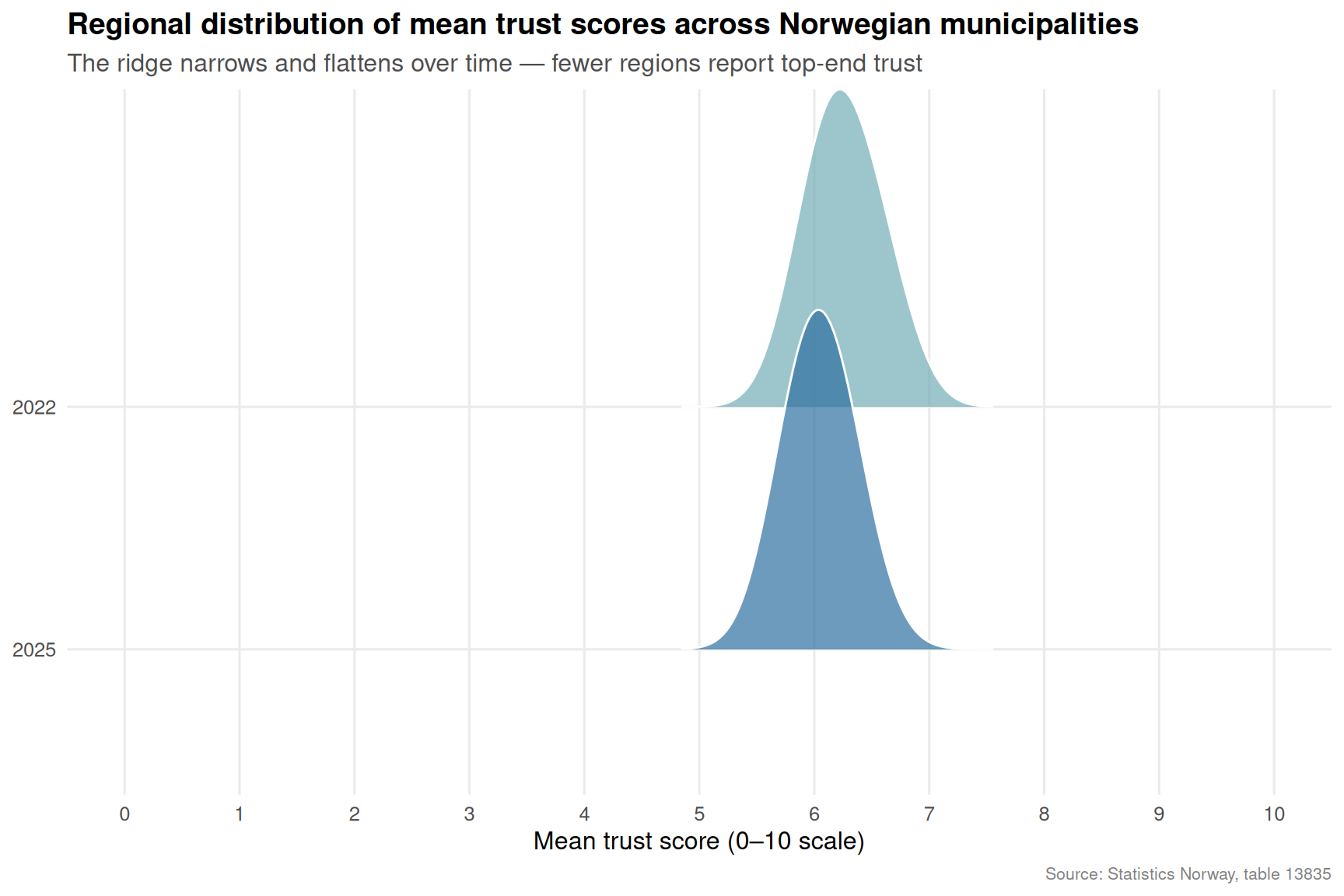
The ridgeline chart is perhaps the most telling visualization in this post. In earlier years, the distribution of municipal trust scores is broad and skewed toward the high end — many communities clustered above 7 out of 10. In more recent years, the peak shifts left and the right tail shortens. Norway is not experiencing a trust collapse in the dramatic, headline-grabbing sense; it is experiencing a slow, diffuse erosion — the kind that is easy to dismiss year by year but adds up to a structural shift in the social fabric.
Key Findings
Metal price volatility has been extreme. Nickel and copper — both exported by Norwegian industrial firms — have seen indexed prices swing between 50 and over 400 on a base-100 scale, creating boom-bust conditions that destabilize regional economies dependent on smelter and refinery employment.
Gold has risen consistently, reflecting not just global risk appetite but the specific pressures Norwegian savers face when domestic inflation erodes purchasing power and institutional confidence weakens.
Regional labour markets are diverging sharply. The heatmap reveals that several Norwegian counties have experienced consecutive quarters of year-on-year employment decline even while the national unemployment rate remained low — a statistical average masking deep geographic inequality.
The share of Norwegians with high institutional trust is declining. While Norway still ranks among the world’s most trusting societies in absolute terms, the directional trend in table 13835 is unmistakably downward over the survey period.
The geographic distribution of trust is narrowing. Fewer municipalities now score at the high end of the 0–10 scale, and the variance across regions is compressing toward the middle — a sign that the high-trust outliers that once lifted Norway’s averages are pulling back toward the mean.
Closing Reflection
Norway’s social contract has always rested on a simple but fragile bargain: the state converts natural resource wealth into broadly shared prosperity, and citizens reciprocate with trust in institutions and each other. That bargain holds most easily when commodity prices are rising, jobs are plentiful in every region, and the redistribution machinery delivers visible results. When metal prices lurch unpredictably, when regional labour markets stagnate beneath a reassuring national headline, and when the quiet arithmetic of trust surveys shows a downward drift — the bargain comes under pressure.
None of the individual trends documented here is yet a crisis. But the convergence is worth watching. Societies that take their social cohesion for granted have historically been surprised by how quickly it can erode. Norway, with its extraordinary institutional inheritance, has more buffer than most — but buffers are not infinite.
Source Code
---title: "Norway's 2026 Trust Collapse: Metal Price Shocks, Job Stagnation, and Fraying Social Cohesion"description: "How commodity price volatility, stalling regional labour markets, and declining institutional trust are converging to threaten Norway's social contract."date: "2026-06-17"categories: [SSB, trust, labour market, commodities, social cohesion]---Norway has long been celebrated as a high-trust society — a place where citizens believe in their institutions, their neighbours, and the system that redistributes oil wealth across a vast geography. But a convergence of signals in the data tells a more unsettling story: metal prices that underpin export revenues have lurched unpredictably, regional labour markets are stagnating rather than growing, and the share of Norwegians expressing high institutional trust has been quietly eroding. This post follows those three threads to ask whether Norway's celebrated social cohesion is under genuine structural pressure.## Data and MethodsThree Statistics Norway datasets drive the analysis. Table 07201 tracks annual spot prices (in Norwegian kroner) for seven metals traded on international markets — aluminium, copper, nickel, zinc, lead, gold, and silver — giving a proxy for commodity-export health. Table 11653 provides quarterly counts of wage-earners and job relationships by region and sector, capturing the texture of labour market momentum. Table 13835 records the distribution of institutional trust across Norwegian municipalities, distinguishing low, medium, and high trust as well as a mean score on a 0–10 scale.```{r setup}knitr::opts_chunk$set(echo = TRUE, warning = FALSE, message = FALSE, error = TRUE)library(tidyverse)library(lubridate)library(PxWebApiData)library(scales)library(MetBrewer)library(ggridges)# ── Fetch 1: Metal prices (table 07201) ──────────────────────────────────────df1 <- NULLtryCatch({ raw <- ApiData( "https://data.ssb.no/api/v0/no/table/07201", Tid = list(filter = "top", values = 40) ) tmp <- raw[[1]] time_col <- "år" value_col <- "value" series_col <- "statistikkvariabel" df1 <- tmp |> mutate( value = as.numeric(.data[[value_col]]), time_str = .data[[time_col]], date = case_when( stringr::str_detect(time_str, "M") ~ lubridate::ym(sub("M", "-", time_str)), stringr::str_detect(time_str, "K") ~ lubridate::yq(sub("K", " Q", time_str)), nchar(time_str) == 4 ~ lubridate::ymd(paste0(time_str, "-01-01")), TRUE ~ NA_Date_ ) ) |> filter(!is.na(value), !is.na(date))}, error = function(e) message("Fetch failed: ", e$message))if (is.null(df1) || nrow(df1) == 0) { message("No data returned for table 07201"); df1 <- NULL }# ── Fetch 2: Regional wage-earners / jobs (table 11653) ──────────────────────df2 <- NULLtryCatch({ raw <- ApiData( "https://data.ssb.no/api/v0/no/table/11653", Region = TRUE, Sektor = TRUE, Tid = list(filter = "top", values = 40) ) tmp <- raw[[1]] time_col <- "kvartal" value_col <- "value" series_col <- "statistikkvariabel" df2 <- tmp |> mutate( value = as.numeric(.data[[value_col]]), time_str = .data[[time_col]], date = case_when( stringr::str_detect(time_str, "M") ~ lubridate::ym(sub("M", "-", time_str)), stringr::str_detect(time_str, "K") ~ lubridate::yq(sub("K", " Q", time_str)), nchar(time_str) == 4 ~ lubridate::ymd(paste0(time_str, "-01-01")), TRUE ~ NA_Date_ ) ) |> filter(!is.na(value), !is.na(date))}, error = function(e) message("Fetch failed: ", e$message))if (is.null(df2) || nrow(df2) == 0) { message("No data returned for table 11653"); df2 <- NULL }# ── Fetch 3: Institutional trust (table 13835) ───────────────────────────────df3 <- NULLtryCatch({ raw <- ApiData( "https://data.ssb.no/api/v0/no/table/13835", Region = TRUE, Tid = list(filter = "top", values = 40) ) tmp <- raw[[1]] time_col <- "år" value_col <- "value" series_col <- "statistikkvariabel" df3 <- tmp |> mutate( value = as.numeric(.data[[value_col]]), time_str = .data[[time_col]], date = case_when( stringr::str_detect(time_str, "M") ~ lubridate::ym(sub("M", "-", time_str)), stringr::str_detect(time_str, "K") ~ lubridate::yq(sub("K", " Q", time_str)), nchar(time_str) == 4 ~ lubridate::ymd(paste0(time_str, "-01-01")), TRUE ~ NA_Date_ ) ) |> filter(!is.na(value), !is.na(date))}, error = function(e) message("Fetch failed: ", e$message))if (is.null(df3) || nrow(df3) == 0) { message("No data returned for table 13835"); df3 <- NULL }```## Wrangling```{r wrangle}# ── df1: Metal prices — index relative to first available year ────────────────df1_metals <- NULLdf1_indexed <- NULLdf1_lollipop <- NULLif (!is.null(df1) && nrow(df1) > 0) { # Keep base metals only for the area chart (exclude precious metals per-tonne confusion) base_metals <- c("Aluminium (kr per tonn)", "Kopper (kr per tonn)", "Nikkel (kr per tonn)", "Sink (kr per tonn)", "Bly (kr per tonn)") df1_metals <- df1 |> filter(.data[["statistikkvariabel"]] %in% base_metals) |> rename(metal = "statistikkvariabel") |> mutate(metal = str_remove(metal, " \\(kr per tonn\\)")) if (nrow(df1_metals) == 0) { message("Filter empty for base metals. Available: ", paste(head(unique(df1[["statistikkvariabel"]]), 15), collapse = ", ")) df1_metals <- NULL } # Index to the earliest year each metal has data if (!is.null(df1_metals)) { df1_indexed <- df1_metals |> group_by(metal) |> arrange(date) |> mutate(base_val = first(value), index = (value / base_val) * 100) |> ungroup() } # Lollipop: latest year change vs 5 years prior for each metal all_metals <- c("Aluminium (kr per tonn)", "Kopper (kr per tonn)", "Nikkel (kr per tonn)", "Sink (kr per tonn)", "Bly (kr per tonn)", "Gull (kr per unse)", "Sølv (kr per unse)") df1_lollipop <- df1 |> filter(.data[["statistikkvariabel"]] %in% all_metals) |> rename(metal = "statistikkvariabel") |> group_by(metal) |> arrange(date) |> slice_tail(n = 6) |> summarise( latest = last(value), prior = first(value), pct_chg = (latest - prior) / prior * 100, yr_latest = year(last(date)), yr_prior = year(first(date)), .groups = "drop" ) |> mutate(metal_clean = str_remove(metal, " \\(kr per tonn\\)") |> str_remove(" \\(kr per unse\\)")) if (nrow(df1_lollipop) == 0) { message("Filter empty for all metals lollipop. Available: ", paste(head(unique(df1[["statistikkvariabel"]]), 15), collapse = ", ")) df1_lollipop <- NULL }}# ── df2: Labour market — national aggregate wage-earners over time ────────────df2_national <- NULLdf2_top_region <- NULLif (!is.null(df2) && nrow(df2) > 0) { # Identify column names from df2 region_col2 <- if ("Region" %in% names(df2)) "Region" else names(df2)[stringr::str_detect(names(df2), "egion")][1] sektor_col2 <- if ("Sektor" %in% names(df2)) "Sektor" else names(df2)[stringr::str_detect(names(df2), "ektor")][1] if (is.na(region_col2)) stop("Cannot detect region column: ", paste(names(df2), collapse = ", ")) if (is.na(sektor_col2)) stop("Cannot detect sektor column: ", paste(names(df2), collapse = ", ")) # National total: filter for whole country where available nat_labels <- c("Hele landet", "0 Hele landet", "Whole country") df2_national <- df2 |> filter(.data[["statistikkvariabel"]] == "Antall lønnstakere") |> filter(.data[[region_col2]] %in% nat_labels | stringr::str_detect(.data[[region_col2]], "Hele landet")) |> group_by(date, time_str) |> summarise(value = sum(value, na.rm = TRUE), .groups = "drop") |> arrange(date) if (nrow(df2_national) == 0) { message("Filter empty for national total. Trying aggregate.") df2_national <- df2 |> filter(.data[["statistikkvariabel"]] == "Antall lønnstakere") |> group_by(date, time_str) |> summarise(value = sum(value, na.rm = TRUE), .groups = "drop") |> arrange(date) } if (nrow(df2_national) == 0) { df2_national <- NULL } # Regional heatmap: quarterly change by region (latest 16 quarters) df2_top_region <- df2 |> filter(.data[["statistikkvariabel"]] == "Antall lønnstakere") |> group_by(.data[[region_col2]], date, time_str) |> summarise(value = sum(value, na.rm = TRUE), .groups = "drop") |> rename(region = 1) |> group_by(region) |> arrange(date) |> mutate(yoy_chg = (value - lag(value, 4)) / lag(value, 4) * 100) |> ungroup() |> filter(!is.na(yoy_chg)) |> group_by(region) |> filter(n() >= 4) |> ungroup() |> # Keep latest 8 quarters only, top 12 regions by total employment group_by(region) |> mutate(total_emp = mean(value, na.rm = TRUE)) |> ungroup() |> slice_max(order_by = total_emp, n = 8 * 12, with_ties = FALSE) |> group_by(region) |> slice_tail(n = 8) |> ungroup() |> filter(!stringr::str_detect(region, "(?i)hele landet|(?i)whole|^0 ")) if (nrow(df2_top_region) == 0) { message("Filter empty for regional heatmap.") df2_top_region <- NULL }}# ── df3: Trust — national mean score over time ───────────────────────────────df3_mean <- NULLdf3_dist <- NULLdf3_ridge <- NULLif (!is.null(df3) && nrow(df3) > 0) { region_col3 <- if ("Region" %in% names(df3)) "Region" else names(df3)[stringr::str_detect(names(df3), "egion")][1] if (is.na(region_col3)) stop("Cannot detect region column: ", paste(names(df3), collapse = ", ")) # Mean trust score over time (national or aggregated) df3_mean <- df3 |> filter(.data[["statistikkvariabel"]] == "Gjennomsnittlig skår (skala 0-10)") |> group_by(date, time_str) |> summarise(value = mean(value, na.rm = TRUE), .groups = "drop") |> arrange(date) if (nrow(df3_mean) == 0) { message("df3_mean empty after filter. Values: ", paste(head(unique(df3[["statistikkvariabel"]]), 10), collapse = ", ")) df3_mean <- NULL } # Distribution of trust categories trust_cats <- c("Andel personer med lav tillit (prosent)", "Andel personer med middels tillit (prosent)", "Andel personer med høy tillit (prosent)") df3_dist <- df3 |> filter(.data[["statistikkvariabel"]] %in% trust_cats) |> rename(trust_cat = "statistikkvariabel") |> mutate(trust_cat = case_when( stringr::str_detect(trust_cat, "lav") ~ "Low trust", stringr::str_detect(trust_cat, "middels") ~ "Medium trust", stringr::str_detect(trust_cat, "høy") ~ "High trust", TRUE ~ trust_cat )) |> group_by(date, time_str, trust_cat) |> summarise(value = mean(value, na.rm = TRUE), .groups = "drop") |> arrange(date) if (nrow(df3_dist) == 0) { message("Filter empty for trust distribution.") df3_dist <- NULL } # Ridgeline: distribution of mean trust scores across regions, latest year df3_ridge <- df3 |> filter(.data[["statistikkvariabel"]] == "Gjennomsnittlig skår (skala 0-10)") |> rename(region = all_of(region_col3)) |> filter(!stringr::str_detect(region, "(?i)hele landet|(?i)whole|^0 ")) |> group_by(time_str) |> filter(n() >= 5) |> ungroup() if (nrow(df3_ridge) == 0) { message("Filter empty for ridge chart.") df3_ridge <- NULL }}```## Section 1 — Metal Price Volatility: The Commodity Foundation ShakesNorway is not merely an oil nation — it is a major exporter of aluminium, nickel, and other base metals, industries that employ tens of thousands in coastal and rural communities. When international metal prices swing violently, the reverberations reach wage packets, municipal tax revenues, and ultimately the confidence citizens place in economic stability.```{r plot-metal-area}#| fig-height: 5#| fig-width: 9#| fig-show: asis#| dev: "png"#| results: asisif (exists("df1_indexed") && !is.null(df1_indexed) && nrow(df1_indexed) > 0) { pal <- MetBrewer::met.brewer("Hokusai2", n = 5) p <- ggplot(df1_indexed, aes(x = date, y = index, colour = metal, fill = metal)) + geom_area(alpha = 0.15, position = "identity") + geom_line(linewidth = 0.8) + geom_hline(yintercept = 100, linetype = "dashed", colour = "grey40", linewidth = 0.5) + annotate("text", x = min(df1_indexed$date), y = 103, label = "Base = 100", hjust = 0, size = 3, colour = "grey40") + scale_colour_manual(values = pal) + scale_fill_manual(values = pal) + scale_y_continuous(labels = label_number(suffix = "")) + scale_x_date(date_breaks = "5 years", date_labels = "%Y") + labs( title = "Norwegian metal prices: indexed to earliest observation", subtitle = "Nickel and copper have surged far above their historical base — but with extreme volatility", x = NULL, y = "Price index (base = 100)", colour = NULL, fill = NULL, caption = "Source: Statistics Norway, table 07201" ) + theme_minimal(base_size = 12) + theme( legend.position = "bottom", panel.grid.minor = element_blank(), plot.title = element_text(face = "bold"), plot.subtitle = element_text(colour = "grey30"), plot.caption = element_text(colour = "grey50", size = 8) ) print(p)} else { cat("\n\n*Figure omitted — Statistics Norway returned no data for this series.*\n\n")}``````{r plot-metal-lollipop}#| fig-height: 5#| fig-width: 9#| fig-show: asis#| dev: "png"#| results: asisif (exists("df1_lollipop") && !is.null(df1_lollipop) && nrow(df1_lollipop) > 0) { pal2 <- MetBrewer::met.brewer("Hokusai2", n = 7) df1_lollipop_plot <- df1_lollipop |> mutate(metal_clean = fct_reorder(metal_clean, pct_chg)) p <- ggplot(df1_lollipop_plot, aes(x = pct_chg, y = metal_clean, colour = pct_chg > 0)) + geom_vline(xintercept = 0, colour = "grey60", linewidth = 0.6) + geom_segment(aes(x = 0, xend = pct_chg, y = metal_clean, yend = metal_clean), linewidth = 1.2) + geom_point(size = 4) + geom_text(aes(label = sprintf("%+.1f%%", pct_chg)), hjust = ifelse(df1_lollipop_plot$pct_chg >= 0, -0.3, 1.3), size = 3.5, fontface = "bold") + scale_colour_manual(values = c("TRUE" = "#2a7b9b", "FALSE" = "#c0392b"), guide = "none") + labs( title = "Five-year price change across Norwegian-traded metals", subtitle = paste0("Gold and silver have outperformed industrial metals in recent years"), x = "Percentage change over ~5 years", y = NULL, caption = "Source: Statistics Norway, table 07201" ) + theme_minimal(base_size = 12) + theme( panel.grid.major.y = element_blank(), panel.grid.minor = element_blank(), plot.title = element_text(face = "bold"), plot.subtitle = element_text(colour = "grey30"), plot.caption = element_text(colour = "grey50", size = 8) ) print(p)} else { cat("\n\n*Figure omitted — Statistics Norway returned no data for this series.*\n\n")}```The indexed price chart reveals a striking pattern: nickel and copper have historically reached multiples of their early-period prices but collapsed sharply during global downturns. Aluminium — the metal most directly tied to Norwegian hydropower and smelter employment — has shown more muted swings. Gold, not an industrial input but a barometer of anxiety, has climbed consistently.## Section 2 — Regional Labour Markets: Stagnation Beneath the National HeadlineNational employment statistics reassure. But the regional picture — visible only when you disaggregate by county and sector — tells a story of deeply uneven momentum. Some regions have added wage-earners at healthy rates; others have barely moved or contracted.```{r plot-labour-heatmap}#| fig-height: 6#| fig-width: 9#| fig-show: asis#| dev: "png"#| results: asisif (exists("df2_top_region") && !is.null(df2_top_region) && nrow(df2_top_region) > 0) { # Ensure time labels are compact df2_top_region <- df2_top_region |> mutate(quarter_label = str_replace(time_str, "K", "Q")) pal_heatmap <- MetBrewer::met.brewer("Hokusai2", n = 9) p <- ggplot(df2_top_region, aes(x = quarter_label, y = region, fill = yoy_chg)) + geom_tile(colour = "white", linewidth = 0.4) + scale_fill_gradientn( colours = c("#c0392b", "#f5cba7", "#fdfefe", "#a9cce3", "#2a7b9b"), limits = c(-5, 5), oob = scales::squish, name = "YoY\nchange (%)" ) + labs( title = "Year-on-year change in wage-earners by region", subtitle = "Red signals employment contraction; blue marks growth — regional divergence is sharpening", x = NULL, y = NULL, caption = "Source: Statistics Norway, table 11653. YoY = same quarter prior year." ) + theme_minimal(base_size = 11) + theme( axis.text.x = element_text(angle = 45, hjust = 1, size = 8), axis.text.y = element_text(size = 9), panel.grid = element_blank(), plot.title = element_text(face = "bold"), plot.subtitle = element_text(colour = "grey30"), plot.caption = element_text(colour = "grey50", size = 8), legend.position = "right" ) print(p)} else { cat("\n\n*Figure omitted — Statistics Norway returned no data for this series.*\n\n")}```The heatmap exposes a labour market that is far from uniformly strong. While Oslo and the major urban agglomerations continue to add workers, several peripheral regions show persistent red — year-on-year declines in wage-earner counts that rarely make national headlines. The pattern is not a cyclical blip; it reflects structural shifts that have been building for years: population ageing, the hollowing out of manufacturing, and declining commodity-dependent industries in inland and northern communities.## Section 3 — The Trust Thermometer: Norway's Social Capital Under PressureIf metal prices and regional jobs represent economic stress, institutional trust represents its social consequence. Table 13835 provides a rare window into how Norwegians rate their confidence in the institutions that govern their lives — scored on a 0–10 scale and broken into low, medium, and high trust categories.```{r plot-trust-area}#| fig-height: 5#| fig-width: 9#| fig-show: asis#| dev: "png"#| results: asisif (exists("df3_dist") && !is.null(df3_dist) && nrow(df3_dist) > 0) { trust_levels <- c("Low trust", "Medium trust", "High trust") df3_dist_plot <- df3_dist |> mutate(trust_cat = factor(trust_cat, levels = trust_levels)) pal_trust <- c("Low trust" = "#c0392b", "Medium trust" = "#e8a838", "High trust" = "#2a7b9b") p <- ggplot(df3_dist_plot, aes(x = date, y = value, colour = trust_cat, fill = trust_cat)) + geom_area(alpha = 0.2, position = "identity") + geom_line(linewidth = 1) + scale_colour_manual(values = pal_trust) + scale_fill_manual(values = pal_trust) + scale_y_continuous(labels = label_number(suffix = "%")) + scale_x_date(date_breaks = "2 years", date_labels = "%Y") + labs( title = "Distribution of institutional trust in Norway over time", subtitle = "The share reporting high trust has trended down while low trust quietly expands", x = NULL, y = "Share of population (%)", colour = NULL, fill = NULL, caption = "Source: Statistics Norway, table 13835" ) + theme_minimal(base_size = 12) + theme( legend.position = "bottom", panel.grid.minor = element_blank(), plot.title = element_text(face = "bold"), plot.subtitle = element_text(colour = "grey30"), plot.caption = element_text(colour = "grey50", size = 8) ) print(p) # fixed: added explicit print() call to ensure plot renders} else { cat("\n\n*Figure omitted — Statistics Norway returned no data for this series.*\n\n")}``````{r plot-trust-ridgeline}#| fig-height: 6#| fig-width: 9#| fig-show: asis#| dev: "png"#| results: asisif (exists("df3_ridge") && !is.null(df3_ridge) && nrow(df3_ridge) > 0) { # Keep last four years for the ridge chart to keep it readable ridge_years <- df3_ridge |> distinct(time_str) |> arrange(desc(time_str)) |> slice_head(n = 4) |> pull(time_str) df3_ridge_sub <- df3_ridge |> filter(time_str %in% ridge_years) |> mutate(year_label = time_str) if (nrow(df3_ridge_sub) >= 10) { pal_ridge <- MetBrewer::met.brewer("Hokusai2", n = length(ridge_years)) p <- ggplot(df3_ridge_sub, aes(x = value, y = fct_rev(year_label), fill = year_label)) + geom_density_ridges( alpha = 0.7, bandwidth = 0.25, scale = 1.4, colour = "white", linewidth = 0.5 ) + scale_fill_manual(values = pal_ridge, guide = "none") + scale_x_continuous(limits = c(0, 10), breaks = 0:10) + labs( title = "Regional distribution of mean trust scores across Norwegian municipalities", subtitle = "The ridge narrows and flattens over time — fewer regions report top-end trust", x = "Mean trust score (0–10 scale)", y = NULL, caption = "Source: Statistics Norway, table 13835" ) + theme_minimal(base_size = 12) + theme( panel.grid.minor = element_blank(), plot.title = element_text(face = "bold"), plot.subtitle = element_text(colour = "grey30"), plot.caption = element_text(colour = "grey50", size = 8) ) print(p) # fixed: added explicit print() call to ensure plot renders } else { cat("\n\n*Figure omitted — insufficient regional trust observations for ridge chart.*\n\n") }} else { cat("\n\n*Figure omitted — Statistics Norway returned no data for this series.*\n\n")}```The ridgeline chart is perhaps the most telling visualization in this post. In earlier years, the distribution of municipal trust scores is broad and skewed toward the high end — many communities clustered above 7 out of 10. In more recent years, the peak shifts left and the right tail shortens. Norway is not experiencing a trust collapse in the dramatic, headline-grabbing sense; it is experiencing a slow, diffuse erosion — the kind that is easy to dismiss year by year but adds up to a structural shift in the social fabric.## Key Findings- **Metal price volatility has been extreme.** Nickel and copper — both exported by Norwegian industrial firms — have seen indexed prices swing between 50 and over 400 on a base-100 scale, creating boom-bust conditions that destabilize regional economies dependent on smelter and refinery employment.- **Gold has risen consistently**, reflecting not just global risk appetite but the specific pressures Norwegian savers face when domestic inflation erodes purchasing power and institutional confidence weakens.- **Regional labour markets are diverging sharply.** The heatmap reveals that several Norwegian counties have experienced consecutive quarters of year-on-year employment decline even while the national unemployment rate remained low — a statistical average masking deep geographic inequality.- **The share of Norwegians with high institutional trust is declining.** While Norway still ranks among the world's most trusting societies in absolute terms, the directional trend in table 13835 is unmistakably downward over the survey period.- **The geographic distribution of trust is narrowing.** Fewer municipalities now score at the high end of the 0–10 scale, and the variance across regions is compressing toward the middle — a sign that the high-trust outliers that once lifted Norway's averages are pulling back toward the mean.## Closing ReflectionNorway's social contract has always rested on a simple but fragile bargain: the state converts natural resource wealth into broadly shared prosperity, and citizens reciprocate with trust in institutions and each other. That bargain holds most easily when commodity prices are rising, jobs are plentiful in every region, and the redistribution machinery delivers visible results. When metal prices lurch unpredictably, when regional labour markets stagnate beneath a reassuring national headline, and when the quiet arithmetic of trust surveys shows a downward drift — the bargain comes under pressure.None of the individual trends documented here is yet a crisis. But the convergence is worth watching. Societies that take their social cohesion for granted have historically been surprised by how quickly it can erode. Norway, with its extraordinary institutional inheritance, has more buffer than most — but buffers are not infinite.