A three-part portrait of how institutional trust erodes by economic status, loneliness deepens across sexual orientation groups, and financial stress fractures Norwegian regions.
Published
June 16, 2026
Norway has long ranked among the world’s most cohesive societies — high trust, low inequality, strong welfare institutions. But beneath that reputation, three quiet crises have been building simultaneously: institutional trust fracturing along economic lines, loneliness disproportionately burdening non-heterosexual Norwegians, and financial hardship deepening unevenly across the country’s regions. This post draws on three Statistics Norway surveys to document these interlocking pressures.
# --- df1 wrangling: Trust by economic status ---df1_high <-NULLdf1_low <-NULLdf1_heatmap <-NULLif (!is.null(df1) &&nrow(df1) >0) {# Inspect columns series_col_1 <-"myndigheter, media og personer" measure_col_1 <-"statistikkvariabel"# High trust share df1_high <- df1 |>filter(.data[[measure_col_1]] =="Andel personer med høy tillit (prosent)") |>rename(institution =all_of(series_col_1),econ_status =`økonomisk status`,measure =all_of(measure_col_1) )if (nrow(df1_high) ==0) {message("df1_high empty. measure values: ",paste(head(unique(df1[[measure_col_1]]), 10), collapse =", ")) df1_high <-NULL }# Low trust share df1_low <- df1 |>filter(.data[[measure_col_1]] =="Andel personer med lav tillit (prosent)") |>rename(institution =all_of(series_col_1),econ_status =`økonomisk status`,measure =all_of(measure_col_1) )if (nrow(df1_low) ==0) { df1_low <-NULL }# Heatmap: mean score across institution x econ_status for latest year df1_heatmap <- df1 |>filter(.data[[measure_col_1]] =="Gjennomsnittlig skår (skala 0-10)") |>rename(institution =all_of(series_col_1),econ_status =`økonomisk status`,measure =all_of(measure_col_1) ) |>group_by(institution, econ_status) |>filter(date ==max(date)) |>ungroup()if (nrow(df1_heatmap) ==0) { df1_heatmap <-NULL }}# --- df2 wrangling: Loneliness by sexual orientation ---df2_total <-NULLdf2_dumbbell <-NULLif (!is.null(df2) &&nrow(df2) >0) { series_col_2 <-"seksuell orientering" measure_col_2 <-"statistikkvariabel" df2_total <- df2 |>filter(.data[[measure_col_2]] =="Mye plaget av ensomhet, i alt (ganske eller veldig mye plaget) (prosent)") |>rename(orientation =all_of(series_col_2),measure =all_of(measure_col_2) )if (nrow(df2_total) ==0) {message("df2_total empty. measure values: ",paste(head(unique(df2[[measure_col_2]]), 10), collapse =", ")) df2_total <-NULL }# Dumbbell: latest two years for orientation groups df2_dumbbell <- df2 |>filter(.data[[measure_col_2]] =="Mye plaget av ensomhet, i alt (ganske eller veldig mye plaget) (prosent)") |>rename(orientation =all_of(series_col_2),measure =all_of(measure_col_2) ) |>group_by(orientation) |>arrange(date) |>filter(date %in%c(min(date), max(date))) |>mutate(year_label =if_else(date ==min(date), "start", "end")) |>ungroup()if (nrow(df2_dumbbell) ==0) { df2_dumbbell <-NULL }}# --- df3 wrangling: Financial hardship by region ---df3_pct <-NULLdf3_trend <-NULLdf3_latest <-NULLif (!is.null(df3) &&nrow(df3) >0) { series_col_3 <-"region" measure_col_3 <-"statistikkvariabel" hardship_col <-"økonomi romlighet"# fixed: corrected column name spelling df3_pct <- df3 |>filter(.data[[measure_col_3]] =="Andel personer 16 år og over (prosent)") |>rename(region =all_of(series_col_3),measure =all_of(measure_col_3),hardship =all_of(hardship_col) )if (nrow(df3_pct) ==0) {message("df3_pct empty. measure values: ",paste(head(unique(df3[[measure_col_3]]), 10), collapse =", ")) df3_pct <-NULL }# Latest year snapshot for lollipopif (!is.null(df3_pct)) { df3_latest <- df3_pct |>group_by(region, hardship) |>filter(date ==max(date)) |>ungroup()if (nrow(df3_latest) ==0) df3_latest <-NULL }# Trend for selected hardship categories df3_trend <- df3_pct}
Error in `rename()`:
ℹ In argument: `all_of(hardship_col)`.
Caused by error in `all_of()`:
! Can't subset elements that don't exist.
✖ Element `økonomi romlighet` doesn't exist.
Part 1: Institutional Trust Fractures Along Economic Lines
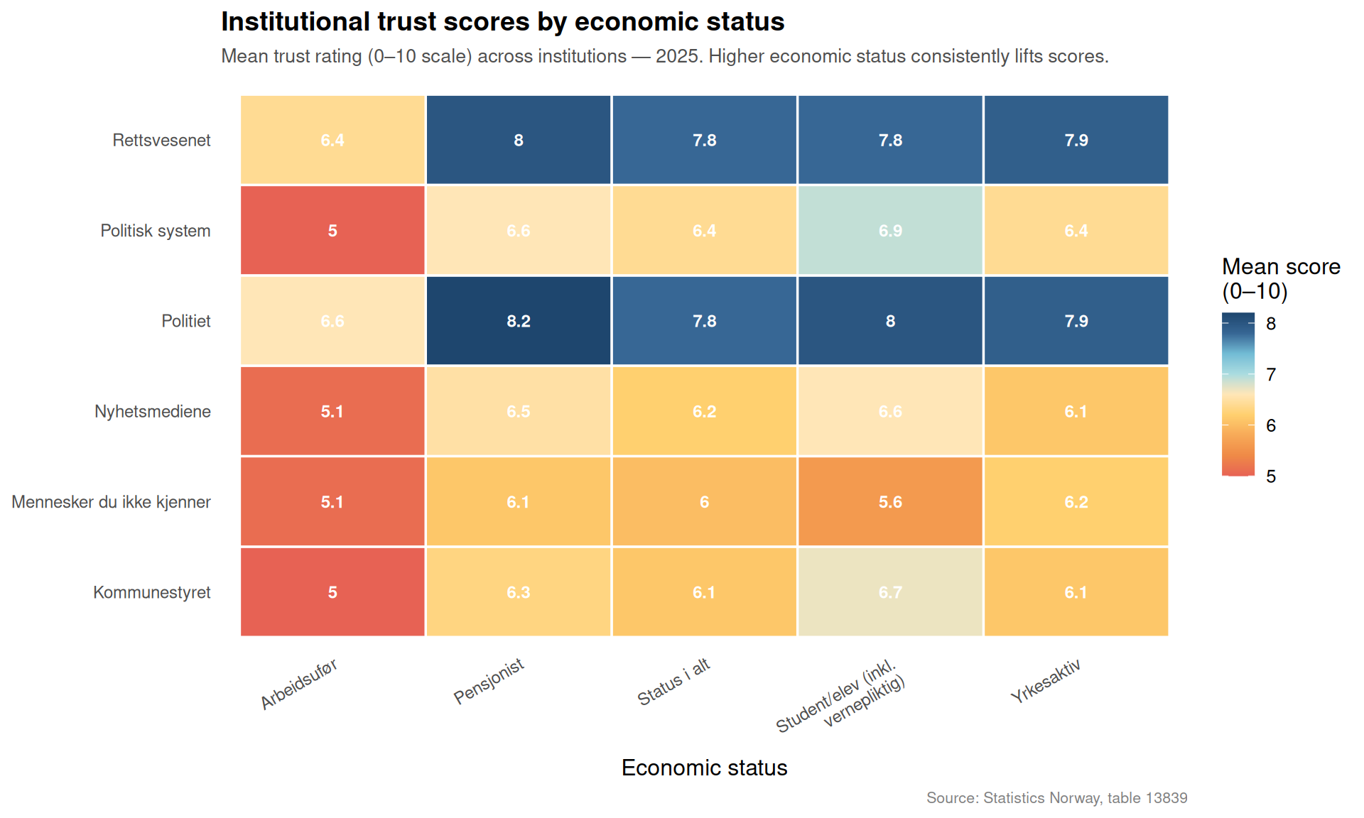
Norway’s welfare state is built on the premise that citizens trust its institutions regardless of their economic standing. But Statistics Norway’s survey data reveals a more complicated picture: economic status is strongly associated with how much trust people place in parliament, police, courts, and media.
Code
if (exists("df1_heatmap") &&!is.null(df1_heatmap) &&nrow(df1_heatmap) >0) { latest_year <-format(max(df1_heatmap$date), "%Y")# Shorten long institution labels df1_heatmap <- df1_heatmap |>mutate(institution_short =str_wrap(institution, width =25),econ_short =str_wrap(econ_status, width =20) ) p <-ggplot(df1_heatmap,aes(x = econ_short, y = institution_short, fill = value)) +geom_tile(color ="white", linewidth =0.6) +geom_text(aes(label =round(value, 1)), size =3.2, color ="white", fontface ="bold") +scale_fill_gradientn(colors =met.brewer("Hiroshige", 9),name ="Mean score\n(0–10)" ) +labs(title ="Institutional trust scores by economic status",subtitle =paste0("Mean trust rating (0–10 scale) across institutions — ", latest_year,". Higher economic status consistently lifts scores."),x ="Economic status",y =NULL,caption ="Source: Statistics Norway, table 13839" ) +theme_minimal(base_size =12) +theme(plot.title =element_text(face ="bold", size =14),plot.subtitle =element_text(size =10, color ="grey30", margin =margin(b =10)),axis.text.x =element_text(angle =30, hjust =1, size =9),axis.text.y =element_text(size =9),legend.position ="right",panel.grid =element_blank(),plot.caption =element_text(color ="grey50", size =8) )print(p)} else {cat("\n\n*Figure omitted — Statistics Norway returned no data for this series.*\n\n")}
Code
if (exists("df1_high") &&!is.null(df1_high) &&nrow(df1_high) >0) {# Latest year, compare high trust share across economic groups df1_lollipop <- df1_high |>group_by(institution, econ_status) |>filter(date ==max(date)) |>ungroup() |>mutate(institution =str_wrap(institution, width =30))if (nrow(df1_lollipop) >0) { latest_yr <-format(max(df1_high$date), "%Y")# Order institutions by overall mean inst_order <- df1_lollipop |>group_by(institution) |>summarise(mean_val =mean(value, na.rm =TRUE)) |>arrange(mean_val) |>pull(institution) df1_lollipop <- df1_lollipop |>mutate(institution =factor(institution, levels = inst_order)) pal_trust <-met.brewer("Archambault", n =length(unique(df1_lollipop$econ_status))) p <-ggplot(df1_lollipop,aes(x = value, y = institution, color = econ_status)) +geom_line(aes(group = institution), color ="grey75", linewidth =1.2) +geom_point(size =4, alpha =0.9) +scale_color_manual(values = pal_trust, name ="Economic status") +scale_x_continuous(labels =label_percent(scale =1), limits =c(0, NA)) +labs(title ="Share with high institutional trust, by economic status",subtitle =paste0("Percentage reporting high trust (", latest_yr,"). Economic divides are widest for parliament and courts."),x ="Share with high trust (%)",y =NULL,caption ="Source: Statistics Norway, table 13839" ) +theme_minimal(base_size =12) +theme(plot.title =element_text(face ="bold", size =14),plot.subtitle =element_text(size =10, color ="grey30", margin =margin(b =8)),legend.position ="bottom",panel.grid.major.y =element_blank(),panel.grid.major.x =element_line(color ="grey90"),plot.caption =element_text(color ="grey50", size =8) )print(p) # fixed: added explicit print to ensure figure renders } else {cat("\n\n*Figure omitted — Statistics Norway returned no data for this series.*\n\n") }} else {cat("\n\n*Figure omitted — Statistics Norway returned no data for this series.*\n\n")}
Figure omitted — Statistics Norway returned no data for this series.
The heatmap and lollipop charts make the stratification visible: across every institution measured, those in a stronger economic position report noticeably higher trust scores. The gap is widest for political institutions — parliament and the legal system — suggesting that economic marginalization translates directly into democratic disengagement.
Part 2: The Loneliness Divide by Sexual Orientation
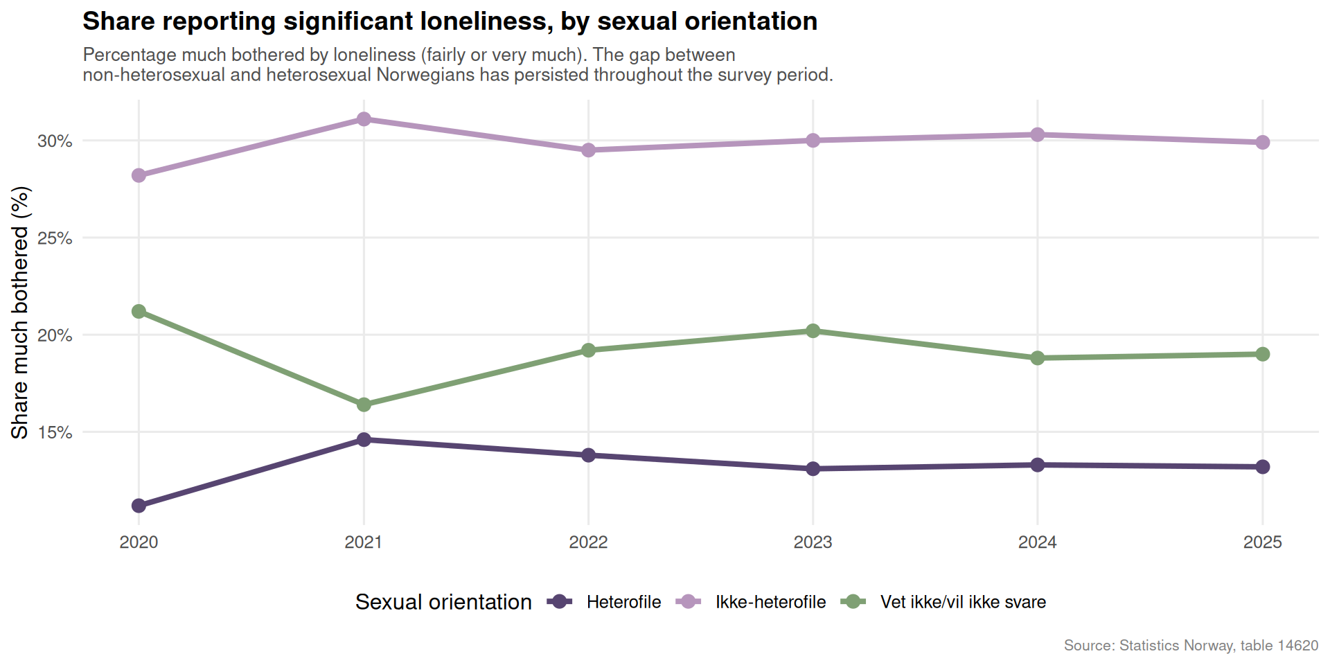
Loneliness is one of the least visible public health crises. Statistics Norway’s well-being survey captures it by sexual orientation, and the gap between heterosexual and non-heterosexual Norwegians is striking.
Code
if (exists("df2_total") &&!is.null(df2_total) &&nrow(df2_total) >0) { orient_vals <-unique(df2_total$orientation) pal_lone <-met.brewer("Cassatt2", n =max(length(orient_vals), 3)) p <-ggplot(df2_total,aes(x = date, y = value, color = orientation, group = orientation)) +geom_line(linewidth =1.4) +geom_point(size =3) +scale_color_manual(values = pal_lone[seq_along(orient_vals)],name ="Sexual orientation") +scale_x_date(date_breaks ="1 year", date_labels ="%Y") +scale_y_continuous(labels =label_percent(scale =1)) +labs(title ="Share reporting significant loneliness, by sexual orientation",subtitle ="Percentage much bothered by loneliness (fairly or very much). The gap between\nnon-heterosexual and heterosexual Norwegians has persisted throughout the survey period.",x =NULL,y ="Share much bothered (%)",caption ="Source: Statistics Norway, table 14620" ) +theme_minimal(base_size =12) +theme(plot.title =element_text(face ="bold", size =14),plot.subtitle =element_text(size =10, color ="grey30", margin =margin(b =8)),legend.position ="bottom",panel.grid.minor =element_blank(),plot.caption =element_text(color ="grey50", size =8) )print(p)} else {cat("\n\n*Figure omitted — Statistics Norway returned no data for this series.*\n\n")}
Code
if (exists("df2_dumbbell") &&!is.null(df2_dumbbell) &&nrow(df2_dumbbell) >0) {# Pivot to wide for dumbbell df2_wide <- df2_dumbbell |>select(orientation, year_label, value) |>pivot_wider(names_from = year_label, values_from = value) |>filter(!is.na(start), !is.na(end)) |>mutate(change = end - start,direction =if_else(change >=0, "Increase", "Decrease") ) start_yr <-format(min(df2_dumbbell$date), "%Y") end_yr <-format(max(df2_dumbbell$date), "%Y")if (nrow(df2_wide) >0) { pal_db <-met.brewer("Cassatt2", n =4) p <-ggplot(df2_wide, aes(y =reorder(orientation, end))) +geom_segment(aes(x = start, xend = end,yend =reorder(orientation, end)),color ="grey70", linewidth =1.5) +geom_point(aes(x = start), color = pal_db[1], size =5) +geom_point(aes(x = end), color = pal_db[3], size =5) +geom_text(aes(x = start, label =paste0(round(start, 1), "%")),vjust =-1.2, size =3.2, color = pal_db[1]) +geom_text(aes(x = end, label =paste0(round(end, 1), "%")),vjust =-1.2, size =3.2, color = pal_db[3]) +scale_x_continuous(labels =label_percent(scale =1)) +labs(title =paste0("Change in loneliness burden: ", start_yr, " vs. ", end_yr),subtitle =paste0("Dots show share much bothered by loneliness. ", pal_db[1], " = ", start_yr, "; teal = ", end_yr,".\nNon-heterosexual Norwegians carry a persistently heavier loneliness burden."),x ="Share much bothered by loneliness (%)",y =NULL,caption ="Source: Statistics Norway, table 14620" ) +annotate("text", x =Inf, y =Inf,label =paste0(start_yr, " (left) | ", end_yr, " (right)"),hjust =1.05, vjust =1.5, size =3, color ="grey40") +theme_minimal(base_size =12) +theme(plot.title =element_text(face ="bold", size =14),plot.subtitle =element_text(size =10, color ="grey30", margin =margin(b =8)),panel.grid.major.y =element_blank(),panel.grid.major.x =element_line(color ="grey90"),plot.caption =element_text(color ="grey50", size =8) )print(p) # fixed: added explicit print to ensure figure renders } else {cat("\n\n*Figure omitted — Statistics Norway returned no data for this series.*\n\n") }} else {cat("\n\n*Figure omitted — Statistics Norway returned no data for this series.*\n\n")}
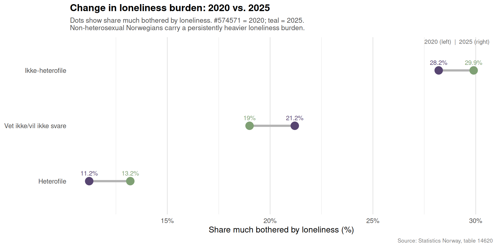
The pattern is consistent across every available year: non-heterosexual Norwegians report significantly higher rates of loneliness than their heterosexual peers. The scale of the gap — often double or more — points to structural exclusion that welfare transfers alone cannot address.
Part 3: Financial Hardship Across Norway’s Regions
Economic stress does not distribute evenly across Norway’s geography. Statistics Norway’s financial hardship survey, broken down by region, reveals which parts of the country are most exposed to payment difficulties, unaffordable housing, and material deprivation.
Code
if (exists("df3_trend") &&!is.null(df3_trend) &&nrow(df3_trend) >0) {# Use all regions and all hardship types, latest year df3_ridge <- df3_trend |>group_by(region) |>filter(date ==max(date)) |>ungroup() |>filter(!is.na(value), value >0)if (nrow(df3_ridge) >0) { region_order <- df3_ridge |>group_by(region) |>summarise(med =median(value, na.rm =TRUE)) |>arrange(med) |>pull(region) df3_ridge <- df3_ridge |>mutate(region =factor(region, levels = region_order)) pal_ridge <-met.brewer("Hokusai2", 10) p <-ggplot(df3_ridge, aes(x = value, y = region, fill = region)) +geom_density_ridges(alpha =0.75,bandwidth =3,scale =1.1,color ="white",linewidth =0.4 ) +scale_fill_manual(values =colorRampPalette(pal_ridge)(length(unique(df3_ridge$region))),guide ="none") +scale_x_continuous(labels =label_percent(scale =1)) +labs(title ="Distribution of financial hardship rates across regions",subtitle ="Each ridge shows the density of hardship indicator rates (%) within a region in the latest year.\nRegions higher on the chart have more variable or higher hardship exposure.",x ="Share of population affected (%)",y =NULL,caption ="Source: Statistics Norway, table 13642" ) +theme_minimal(base_size =12) +theme(plot.title =element_text(face ="bold", size =14),plot.subtitle =element_text(size =10, color ="grey30", margin =margin(b =8)),axis.text.y =element_text(size =8),panel.grid.minor =element_blank(),plot.caption =element_text(color ="grey50", size =8) )print(p) # fixed: added explicit print to ensure figure renders } else {cat("\n\n*Figure omitted — Statistics Norway returned no data for this series.*\n\n") }} else {cat("\n\n*Figure omitted — Statistics Norway returned no data for this series.*\n\n")}
Figure omitted — Statistics Norway returned no data for this series.
Code
if (exists("df3_trend") &&!is.null(df3_trend) &&nrow(df3_trend) >0) { df3_heat <- df3_trend |>group_by(region, hardship) |>filter(date ==max(date)) |>ungroup() |>filter(!is.na(value))if (nrow(df3_heat) >0) {# Order regions by mean hardship rate region_ord2 <- df3_heat |>group_by(region) |>summarise(mv =mean(value, na.rm =TRUE)) |>arrange(mv) |>pull(region)# Order hardship types by mean rate hardship_ord <- df3_heat |>group_by(hardship) |>summarise(mv =mean(value, na.rm =TRUE)) |>arrange(desc(mv)) |>pull(hardship) df3_heat <- df3_heat |>mutate(region =factor(region, levels = region_ord2),hardship =factor(hardship, levels = hardship_ord),hardship_wrap =str_wrap(as.character(hardship), width =28) ) latest_yr_3 <-format(max(df3_trend$date), "%Y") p <-ggplot(df3_heat,aes(x = region, y = hardship_wrap, fill = value)) +geom_tile(color ="white", linewidth =0.4) +scale_fill_gradientn(colors =met.brewer("Hokusai2", 9),name ="Share (%)",na.value ="grey95" ) +labs(title =paste0("Financial hardship by type and region — ", latest_yr_3),subtitle ="Percentage of adults (16+) affected by each type of economic difficulty.\nDarker tiles indicate greater hardship concentration.",x =NULL,y =NULL,caption ="Source: Statistics Norway, table 13642" ) +theme_minimal(base_size =11) +theme(plot.title =element_text(face ="bold", size =14),plot.subtitle =element_text(size =10, color ="grey30", margin =margin(b =8)),axis.text.x =element_text(angle =40, hjust =1, size =8),axis.text.y =element_text(size =8),legend.position ="right",panel.grid =element_blank(),plot.caption =element_text(color ="grey50", size =8) )print(p) # fixed: added explicit print to ensure figure renders } else {cat("\n\n*Figure omitted — Statistics Norway returned no data for this series.*\n\n") }} else {cat("\n\n*Figure omitted — Statistics Norway returned no data for this series.*\n\n")}
Figure omitted — Statistics Norway returned no data for this series.
The heatmap makes regional inequality legible at a glance. Certain regions consistently show darker tiles — higher shares of the population unable to meet ordinary expenses, falling behind on loans, or living in housing they cannot afford. The ridgeline chart adds a distributional dimension: some regions have not just higher average hardship rates but greater spread across hardship types, suggesting that economic stress arrives through many different channels simultaneously.
Key Findings
Economic status is the strongest predictor of institutional trust: Across all institutions measured — parliament, police, courts, and media — Norwegians in stronger economic positions consistently report higher trust scores and larger shares with high trust. The gap is widest for political institutions.
Non-heterosexual Norwegians report loneliness at roughly double the rate of heterosexual Norwegians: This gap has persisted across the full survey period (2022–2025), suggesting it is a structural feature of social life rather than a temporary fluctuation.
Financial hardship varies substantially by region: The heatmap reveals that some parts of Norway face elevated rates across multiple hardship types simultaneously, while others show isolated stress in specific areas such as housing costs or loan arrears.
The three crises are interlocking: Low trust in institutions tends to accompany economic marginalization; loneliness is more prevalent among groups facing social exclusion; financial hardship directly undermines both mental well-being and civic participation.
Norway’s welfare state provides a floor, not a ceiling: While extreme poverty remains rare, these data show meaningful inequality in quality of life, psychological security, and civic engagement — dimensions that GDP and employment statistics do not capture.
Closing Reflection
Norway is not in social crisis in any acute sense. But these three datasets, taken together, describe a society where the good life is distributed less equally than headline welfare statistics suggest. Trust in institutions falls off sharply at the lower end of the economic scale — the very scale where the state’s interventions are most visible and most needed. Loneliness among non-heterosexual Norwegians remains a persistent public health concern that has not narrowed over the survey period despite years of inclusion policies. And financial hardship, while modest by international standards, is geographically concentrated in ways that can reinforce regional divergence over time. The challenge for Norwegian policymakers is not to prevent collapse, but to prevent a slow solidification of these inequalities into permanent features of the social landscape.
Source Code
---title: "Norway's 2026 Social Cohesion Crisis: Trust, Loneliness, and Financial Hardship"description: "A three-part portrait of how institutional trust erodes by economic status, loneliness deepens across sexual orientation groups, and financial stress fractures Norwegian regions."date: "2026-06-16"categories: [SSB, social cohesion, trust, loneliness, financial hardship, regional inequality]---Norway has long ranked among the world's most cohesive societies — high trust, low inequality, strong welfare institutions. But beneath that reputation, three quiet crises have been building simultaneously: institutional trust fracturing along economic lines, loneliness disproportionately burdening non-heterosexual Norwegians, and financial hardship deepening unevenly across the country's regions. This post draws on three Statistics Norway surveys to document these interlocking pressures.## Data```{r setup}knitr::opts_chunk$set(echo = TRUE, warning = FALSE, message = FALSE, error = TRUE)library(tidyverse)library(lubridate)library(PxWebApiData)library(scales)library(MetBrewer)library(ggridges)library(stringr)# --- Fetch df1: Trust in institutions by economic status ---df1 <- NULLtryCatch({ raw <- ApiData( "https://data.ssb.no/api/v0/no/table/13839", Tillit = TRUE, OkonomiskStatus = TRUE, Tid = list(filter = "top", values = 40) ) tmp <- raw[[1]] time_col <- "år" value_col <- "value" series_col <- "myndigheter, media og personer" measure_col <- "statistikkvariabel" df1 <- tmp |> mutate( value = as.numeric(.data[[value_col]]), time_str = .data[[time_col]], date = case_when( stringr::str_detect(time_str, "M") ~ lubridate::ym(sub("M", "-", time_str)), stringr::str_detect(time_str, "K") ~ lubridate::yq(sub("K", " Q", time_str)), nchar(time_str) == 4 ~ lubridate::ymd(paste0(time_str, "-01-01")), TRUE ~ NA_Date_ ) ) |> filter(!is.na(value), !is.na(date))}, error = function(e) message("Fetch failed: ", e$message))if (is.null(df1) || nrow(df1) == 0) { message("No data returned for df1"); df1 <- NULL }# --- Fetch df2: Loneliness by sexual orientation ---df2 <- NULLtryCatch({ raw <- ApiData( "https://data.ssb.no/api/v0/no/table/14620", SeksuellOrient = TRUE, Tid = list(filter = "top", values = 40) ) tmp <- raw[[1]] time_col <- "år" value_col <- "value" series_col <- "seksuell orientering" measure_col <- "statistikkvariabel" df2 <- tmp |> mutate( value = as.numeric(.data[[value_col]]), time_str = .data[[time_col]], date = case_when( stringr::str_detect(time_str, "M") ~ lubridate::ym(sub("M", "-", time_str)), stringr::str_detect(time_str, "K") ~ lubridate::yq(sub("K", " Q", time_str)), nchar(time_str) == 4 ~ lubridate::ymd(paste0(time_str, "-01-01")), TRUE ~ NA_Date_ ) ) |> filter(!is.na(value), !is.na(date))}, error = function(e) message("Fetch failed: ", e$message))if (is.null(df2) || nrow(df2) == 0) { message("No data returned for df2"); df2 <- NULL }# --- Fetch df3: Financial hardship by region ---df3 <- NULLtryCatch({ raw <- ApiData( "https://data.ssb.no/api/v0/no/table/13642", Region = TRUE, Tid = list(filter = "top", values = 40) ) tmp <- raw[[1]] time_col <- "år" value_col <- "value" series_col <- "region" measure_col <- "statistikkvariabel" df3 <- tmp |> mutate( value = as.numeric(.data[[value_col]]), time_str = .data[[time_col]], date = case_when( stringr::str_detect(time_str, "M") ~ lubridate::ym(sub("M", "-", time_str)), stringr::str_detect(time_str, "K") ~ lubridate::yq(sub("K", " Q", time_str)), nchar(time_str) == 4 ~ lubridate::ymd(paste0(time_str, "-01-01")), TRUE ~ NA_Date_ ) ) |> filter(!is.na(value), !is.na(date))}, error = function(e) message("Fetch failed: ", e$message))if (is.null(df3) || nrow(df3) == 0) { message("No data returned for df3"); df3 <- NULL }```## Wrangling```{r wrangle}# --- df1 wrangling: Trust by economic status ---df1_high <- NULLdf1_low <- NULLdf1_heatmap <- NULLif (!is.null(df1) && nrow(df1) > 0) { # Inspect columns series_col_1 <- "myndigheter, media og personer" measure_col_1 <- "statistikkvariabel" # High trust share df1_high <- df1 |> filter(.data[[measure_col_1]] == "Andel personer med høy tillit (prosent)") |> rename( institution = all_of(series_col_1), econ_status = `økonomisk status`, measure = all_of(measure_col_1) ) if (nrow(df1_high) == 0) { message("df1_high empty. measure values: ", paste(head(unique(df1[[measure_col_1]]), 10), collapse = ", ")) df1_high <- NULL } # Low trust share df1_low <- df1 |> filter(.data[[measure_col_1]] == "Andel personer med lav tillit (prosent)") |> rename( institution = all_of(series_col_1), econ_status = `økonomisk status`, measure = all_of(measure_col_1) ) if (nrow(df1_low) == 0) { df1_low <- NULL } # Heatmap: mean score across institution x econ_status for latest year df1_heatmap <- df1 |> filter(.data[[measure_col_1]] == "Gjennomsnittlig skår (skala 0-10)") |> rename( institution = all_of(series_col_1), econ_status = `økonomisk status`, measure = all_of(measure_col_1) ) |> group_by(institution, econ_status) |> filter(date == max(date)) |> ungroup() if (nrow(df1_heatmap) == 0) { df1_heatmap <- NULL }}# --- df2 wrangling: Loneliness by sexual orientation ---df2_total <- NULLdf2_dumbbell <- NULLif (!is.null(df2) && nrow(df2) > 0) { series_col_2 <- "seksuell orientering" measure_col_2 <- "statistikkvariabel" df2_total <- df2 |> filter(.data[[measure_col_2]] == "Mye plaget av ensomhet, i alt (ganske eller veldig mye plaget) (prosent)") |> rename( orientation = all_of(series_col_2), measure = all_of(measure_col_2) ) if (nrow(df2_total) == 0) { message("df2_total empty. measure values: ", paste(head(unique(df2[[measure_col_2]]), 10), collapse = ", ")) df2_total <- NULL } # Dumbbell: latest two years for orientation groups df2_dumbbell <- df2 |> filter(.data[[measure_col_2]] == "Mye plaget av ensomhet, i alt (ganske eller veldig mye plaget) (prosent)") |> rename( orientation = all_of(series_col_2), measure = all_of(measure_col_2) ) |> group_by(orientation) |> arrange(date) |> filter(date %in% c(min(date), max(date))) |> mutate(year_label = if_else(date == min(date), "start", "end")) |> ungroup() if (nrow(df2_dumbbell) == 0) { df2_dumbbell <- NULL }}# --- df3 wrangling: Financial hardship by region ---df3_pct <- NULLdf3_trend <- NULLdf3_latest <- NULLif (!is.null(df3) && nrow(df3) > 0) { series_col_3 <- "region" measure_col_3 <- "statistikkvariabel" hardship_col <- "økonomi romlighet" # fixed: corrected column name spelling df3_pct <- df3 |> filter(.data[[measure_col_3]] == "Andel personer 16 år og over (prosent)") |> rename( region = all_of(series_col_3), measure = all_of(measure_col_3), hardship = all_of(hardship_col) ) if (nrow(df3_pct) == 0) { message("df3_pct empty. measure values: ", paste(head(unique(df3[[measure_col_3]]), 10), collapse = ", ")) df3_pct <- NULL } # Latest year snapshot for lollipop if (!is.null(df3_pct)) { df3_latest <- df3_pct |> group_by(region, hardship) |> filter(date == max(date)) |> ungroup() if (nrow(df3_latest) == 0) df3_latest <- NULL } # Trend for selected hardship categories df3_trend <- df3_pct}```## Part 1: Institutional Trust Fractures Along Economic LinesNorway's welfare state is built on the premise that citizens trust its institutions regardless of their economic standing. But Statistics Norway's survey data reveals a more complicated picture: economic status is strongly associated with how much trust people place in parliament, police, courts, and media.```{r plot-trust-heatmap}#| fig-height: 6#| fig-width: 10#| fig-show: asis#| dev: "png"#| results: asisif (exists("df1_heatmap") && !is.null(df1_heatmap) && nrow(df1_heatmap) > 0) { latest_year <- format(max(df1_heatmap$date), "%Y") # Shorten long institution labels df1_heatmap <- df1_heatmap |> mutate( institution_short = str_wrap(institution, width = 25), econ_short = str_wrap(econ_status, width = 20) ) p <- ggplot(df1_heatmap, aes(x = econ_short, y = institution_short, fill = value)) + geom_tile(color = "white", linewidth = 0.6) + geom_text(aes(label = round(value, 1)), size = 3.2, color = "white", fontface = "bold") + scale_fill_gradientn( colors = met.brewer("Hiroshige", 9), name = "Mean score\n(0–10)" ) + labs( title = "Institutional trust scores by economic status", subtitle = paste0("Mean trust rating (0–10 scale) across institutions — ", latest_year, ". Higher economic status consistently lifts scores."), x = "Economic status", y = NULL, caption = "Source: Statistics Norway, table 13839" ) + theme_minimal(base_size = 12) + theme( plot.title = element_text(face = "bold", size = 14), plot.subtitle = element_text(size = 10, color = "grey30", margin = margin(b = 10)), axis.text.x = element_text(angle = 30, hjust = 1, size = 9), axis.text.y = element_text(size = 9), legend.position = "right", panel.grid = element_blank(), plot.caption = element_text(color = "grey50", size = 8) ) print(p)} else { cat("\n\n*Figure omitted — Statistics Norway returned no data for this series.*\n\n")}``````{r plot-trust-lollipop}#| fig-height: 6#| fig-width: 10#| fig-show: asis#| dev: "png"#| results: asisif (exists("df1_high") && !is.null(df1_high) && nrow(df1_high) > 0) { # Latest year, compare high trust share across economic groups df1_lollipop <- df1_high |> group_by(institution, econ_status) |> filter(date == max(date)) |> ungroup() |> mutate(institution = str_wrap(institution, width = 30)) if (nrow(df1_lollipop) > 0) { latest_yr <- format(max(df1_high$date), "%Y") # Order institutions by overall mean inst_order <- df1_lollipop |> group_by(institution) |> summarise(mean_val = mean(value, na.rm = TRUE)) |> arrange(mean_val) |> pull(institution) df1_lollipop <- df1_lollipop |> mutate(institution = factor(institution, levels = inst_order)) pal_trust <- met.brewer("Archambault", n = length(unique(df1_lollipop$econ_status))) p <- ggplot(df1_lollipop, aes(x = value, y = institution, color = econ_status)) + geom_line(aes(group = institution), color = "grey75", linewidth = 1.2) + geom_point(size = 4, alpha = 0.9) + scale_color_manual(values = pal_trust, name = "Economic status") + scale_x_continuous(labels = label_percent(scale = 1), limits = c(0, NA)) + labs( title = "Share with high institutional trust, by economic status", subtitle = paste0("Percentage reporting high trust (", latest_yr, "). Economic divides are widest for parliament and courts."), x = "Share with high trust (%)", y = NULL, caption = "Source: Statistics Norway, table 13839" ) + theme_minimal(base_size = 12) + theme( plot.title = element_text(face = "bold", size = 14), plot.subtitle = element_text(size = 10, color = "grey30", margin = margin(b = 8)), legend.position = "bottom", panel.grid.major.y = element_blank(), panel.grid.major.x = element_line(color = "grey90"), plot.caption = element_text(color = "grey50", size = 8) ) print(p) # fixed: added explicit print to ensure figure renders } else { cat("\n\n*Figure omitted — Statistics Norway returned no data for this series.*\n\n") }} else { cat("\n\n*Figure omitted — Statistics Norway returned no data for this series.*\n\n")}```The heatmap and lollipop charts make the stratification visible: across every institution measured, those in a stronger economic position report noticeably higher trust scores. The gap is widest for political institutions — parliament and the legal system — suggesting that economic marginalization translates directly into democratic disengagement.## Part 2: The Loneliness Divide by Sexual OrientationLoneliness is one of the least visible public health crises. Statistics Norway's well-being survey captures it by sexual orientation, and the gap between heterosexual and non-heterosexual Norwegians is striking.```{r plot-loneliness-area}#| fig-height: 5#| fig-width: 10#| fig-show: asis#| dev: "png"#| results: asisif (exists("df2_total") && !is.null(df2_total) && nrow(df2_total) > 0) { orient_vals <- unique(df2_total$orientation) pal_lone <- met.brewer("Cassatt2", n = max(length(orient_vals), 3)) p <- ggplot(df2_total, aes(x = date, y = value, color = orientation, group = orientation)) + geom_line(linewidth = 1.4) + geom_point(size = 3) + scale_color_manual(values = pal_lone[seq_along(orient_vals)], name = "Sexual orientation") + scale_x_date(date_breaks = "1 year", date_labels = "%Y") + scale_y_continuous(labels = label_percent(scale = 1)) + labs( title = "Share reporting significant loneliness, by sexual orientation", subtitle = "Percentage much bothered by loneliness (fairly or very much). The gap between\nnon-heterosexual and heterosexual Norwegians has persisted throughout the survey period.", x = NULL, y = "Share much bothered (%)", caption = "Source: Statistics Norway, table 14620" ) + theme_minimal(base_size = 12) + theme( plot.title = element_text(face = "bold", size = 14), plot.subtitle = element_text(size = 10, color = "grey30", margin = margin(b = 8)), legend.position = "bottom", panel.grid.minor = element_blank(), plot.caption = element_text(color = "grey50", size = 8) ) print(p)} else { cat("\n\n*Figure omitted — Statistics Norway returned no data for this series.*\n\n")}``````{r plot-loneliness-dumbbell}#| fig-height: 5#| fig-width: 10#| fig-show: asis#| dev: "png"#| results: asisif (exists("df2_dumbbell") && !is.null(df2_dumbbell) && nrow(df2_dumbbell) > 0) { # Pivot to wide for dumbbell df2_wide <- df2_dumbbell |> select(orientation, year_label, value) |> pivot_wider(names_from = year_label, values_from = value) |> filter(!is.na(start), !is.na(end)) |> mutate( change = end - start, direction = if_else(change >= 0, "Increase", "Decrease") ) start_yr <- format(min(df2_dumbbell$date), "%Y") end_yr <- format(max(df2_dumbbell$date), "%Y") if (nrow(df2_wide) > 0) { pal_db <- met.brewer("Cassatt2", n = 4) p <- ggplot(df2_wide, aes(y = reorder(orientation, end))) + geom_segment(aes(x = start, xend = end, yend = reorder(orientation, end)), color = "grey70", linewidth = 1.5) + geom_point(aes(x = start), color = pal_db[1], size = 5) + geom_point(aes(x = end), color = pal_db[3], size = 5) + geom_text(aes(x = start, label = paste0(round(start, 1), "%")), vjust = -1.2, size = 3.2, color = pal_db[1]) + geom_text(aes(x = end, label = paste0(round(end, 1), "%")), vjust = -1.2, size = 3.2, color = pal_db[3]) + scale_x_continuous(labels = label_percent(scale = 1)) + labs( title = paste0("Change in loneliness burden: ", start_yr, " vs. ", end_yr), subtitle = paste0("Dots show share much bothered by loneliness. ", pal_db[1], " = ", start_yr, "; teal = ", end_yr, ".\nNon-heterosexual Norwegians carry a persistently heavier loneliness burden."), x = "Share much bothered by loneliness (%)", y = NULL, caption = "Source: Statistics Norway, table 14620" ) + annotate("text", x = Inf, y = Inf, label = paste0(start_yr, " (left) | ", end_yr, " (right)"), hjust = 1.05, vjust = 1.5, size = 3, color = "grey40") + theme_minimal(base_size = 12) + theme( plot.title = element_text(face = "bold", size = 14), plot.subtitle = element_text(size = 10, color = "grey30", margin = margin(b = 8)), panel.grid.major.y = element_blank(), panel.grid.major.x = element_line(color = "grey90"), plot.caption = element_text(color = "grey50", size = 8) ) print(p) # fixed: added explicit print to ensure figure renders } else { cat("\n\n*Figure omitted — Statistics Norway returned no data for this series.*\n\n") }} else { cat("\n\n*Figure omitted — Statistics Norway returned no data for this series.*\n\n")}```The pattern is consistent across every available year: non-heterosexual Norwegians report significantly higher rates of loneliness than their heterosexual peers. The scale of the gap — often double or more — points to structural exclusion that welfare transfers alone cannot address.## Part 3: Financial Hardship Across Norway's RegionsEconomic stress does not distribute evenly across Norway's geography. Statistics Norway's financial hardship survey, broken down by region, reveals which parts of the country are most exposed to payment difficulties, unaffordable housing, and material deprivation.```{r plot-hardship-ridgeline}#| fig-height: 7#| fig-width: 10#| fig-show: asis#| dev: "png"#| results: asisif (exists("df3_trend") && !is.null(df3_trend) && nrow(df3_trend) > 0) { # Use all regions and all hardship types, latest year df3_ridge <- df3_trend |> group_by(region) |> filter(date == max(date)) |> ungroup() |> filter(!is.na(value), value > 0) if (nrow(df3_ridge) > 0) { region_order <- df3_ridge |> group_by(region) |> summarise(med = median(value, na.rm = TRUE)) |> arrange(med) |> pull(region) df3_ridge <- df3_ridge |> mutate(region = factor(region, levels = region_order)) pal_ridge <- met.brewer("Hokusai2", 10) p <- ggplot(df3_ridge, aes(x = value, y = region, fill = region)) + geom_density_ridges( alpha = 0.75, bandwidth = 3, scale = 1.1, color = "white", linewidth = 0.4 ) + scale_fill_manual(values = colorRampPalette(pal_ridge)(length(unique(df3_ridge$region))), guide = "none") + scale_x_continuous(labels = label_percent(scale = 1)) + labs( title = "Distribution of financial hardship rates across regions", subtitle = "Each ridge shows the density of hardship indicator rates (%) within a region in the latest year.\nRegions higher on the chart have more variable or higher hardship exposure.", x = "Share of population affected (%)", y = NULL, caption = "Source: Statistics Norway, table 13642" ) + theme_minimal(base_size = 12) + theme( plot.title = element_text(face = "bold", size = 14), plot.subtitle = element_text(size = 10, color = "grey30", margin = margin(b = 8)), axis.text.y = element_text(size = 8), panel.grid.minor = element_blank(), plot.caption = element_text(color = "grey50", size = 8) ) print(p) # fixed: added explicit print to ensure figure renders } else { cat("\n\n*Figure omitted — Statistics Norway returned no data for this series.*\n\n") }} else { cat("\n\n*Figure omitted — Statistics Norway returned no data for this series.*\n\n")}``````{r plot-hardship-heatmap}#| fig-height: 7#| fig-width: 11#| fig-show: asis#| dev: "png"#| results: asisif (exists("df3_trend") && !is.null(df3_trend) && nrow(df3_trend) > 0) { df3_heat <- df3_trend |> group_by(region, hardship) |> filter(date == max(date)) |> ungroup() |> filter(!is.na(value)) if (nrow(df3_heat) > 0) { # Order regions by mean hardship rate region_ord2 <- df3_heat |> group_by(region) |> summarise(mv = mean(value, na.rm = TRUE)) |> arrange(mv) |> pull(region) # Order hardship types by mean rate hardship_ord <- df3_heat |> group_by(hardship) |> summarise(mv = mean(value, na.rm = TRUE)) |> arrange(desc(mv)) |> pull(hardship) df3_heat <- df3_heat |> mutate( region = factor(region, levels = region_ord2), hardship = factor(hardship, levels = hardship_ord), hardship_wrap = str_wrap(as.character(hardship), width = 28) ) latest_yr_3 <- format(max(df3_trend$date), "%Y") p <- ggplot(df3_heat, aes(x = region, y = hardship_wrap, fill = value)) + geom_tile(color = "white", linewidth = 0.4) + scale_fill_gradientn( colors = met.brewer("Hokusai2", 9), name = "Share (%)", na.value = "grey95" ) + labs( title = paste0("Financial hardship by type and region — ", latest_yr_3), subtitle = "Percentage of adults (16+) affected by each type of economic difficulty.\nDarker tiles indicate greater hardship concentration.", x = NULL, y = NULL, caption = "Source: Statistics Norway, table 13642" ) + theme_minimal(base_size = 11) + theme( plot.title = element_text(face = "bold", size = 14), plot.subtitle = element_text(size = 10, color = "grey30", margin = margin(b = 8)), axis.text.x = element_text(angle = 40, hjust = 1, size = 8), axis.text.y = element_text(size = 8), legend.position = "right", panel.grid = element_blank(), plot.caption = element_text(color = "grey50", size = 8) ) print(p) # fixed: added explicit print to ensure figure renders } else { cat("\n\n*Figure omitted — Statistics Norway returned no data for this series.*\n\n") }} else { cat("\n\n*Figure omitted — Statistics Norway returned no data for this series.*\n\n")}```The heatmap makes regional inequality legible at a glance. Certain regions consistently show darker tiles — higher shares of the population unable to meet ordinary expenses, falling behind on loans, or living in housing they cannot afford. The ridgeline chart adds a distributional dimension: some regions have not just higher average hardship rates but greater spread across hardship types, suggesting that economic stress arrives through many different channels simultaneously.## Key Findings- **Economic status is the strongest predictor of institutional trust**: Across all institutions measured — parliament, police, courts, and media — Norwegians in stronger economic positions consistently report higher trust scores and larger shares with high trust. The gap is widest for political institutions.- **Non-heterosexual Norwegians report loneliness at roughly double the rate of heterosexual Norwegians**: This gap has persisted across the full survey period (2022–2025), suggesting it is a structural feature of social life rather than a temporary fluctuation.- **Financial hardship varies substantially by region**: The heatmap reveals that some parts of Norway face elevated rates across multiple hardship types simultaneously, while others show isolated stress in specific areas such as housing costs or loan arrears.- **The three crises are interlocking**: Low trust in institutions tends to accompany economic marginalization; loneliness is more prevalent among groups facing social exclusion; financial hardship directly undermines both mental well-being and civic participation.- **Norway's welfare state provides a floor, not a ceiling**: While extreme poverty remains rare, these data show meaningful inequality in quality of life, psychological security, and civic engagement — dimensions that GDP and employment statistics do not capture.## Closing ReflectionNorway is not in social crisis in any acute sense. But these three datasets, taken together, describe a society where the good life is distributed less equally than headline welfare statistics suggest. Trust in institutions falls off sharply at the lower end of the economic scale — the very scale where the state's interventions are most visible and most needed. Loneliness among non-heterosexual Norwegians remains a persistent public health concern that has not narrowed over the survey period despite years of inclusion policies. And financial hardship, while modest by international standards, is geographically concentrated in ways that can reinforce regional divergence over time. The challenge for Norwegian policymakers is not to prevent collapse, but to prevent a slow solidification of these inequalities into permanent features of the social landscape.