A data-driven examination of how softening employment, persistent criminal convictions, and stubborn food inflation are testing Norway’s social resilience in 2026.
Published
June 15, 2026
Norway has long projected an image of stability — low unemployment, low crime, and a welfare state that cushions economic shocks. But a closer reading of Statistics Norway’s most recent data tells a more complicated story. Labour force participation is showing signs of fatigue, criminal convictions remain at structurally elevated levels, and food prices continue to squeeze household budgets in ways that official averages tend to obscure.
# --- Labour market derived data ---df1_employed <-NULLdf1_unemployed <-NULLdf1_rate <-NULLdf1_combined <-NULLif (!is.null(df1) &&nrow(df1) >0) { df1_employed <- df1 |>filter(.data[["statistikkvariabel"]] =="Sysselsatte (1000 personer)") |>select(date, time_str, kjønn, alder, value)if (nrow(df1_employed) ==0) {message("df1_employed empty. Values: ",paste(head(unique(df1[["statistikkvariabel"]]), 15), collapse =", ")) df1_employed <-NULL } df1_unemployed <- df1 |>filter(.data[["statistikkvariabel"]] =="Arbeidsledige i prosent av arbeidsstyrken") |>select(date, time_str, kjønn, alder, value)if (nrow(df1_unemployed) ==0) {message("df1_unemployed empty.") df1_unemployed <-NULL }# Combined for area chart: employed + labour force totals df1_combined <- df1 |>filter( .data[["statistikkvariabel"]] %in%c("Sysselsatte (1000 personer)","Arbeidsstyrken (1000 personer)" ) ) |>group_by(date, statistikkvariabel) |>summarise(value =sum(value, na.rm =TRUE), .groups ="drop")if (nrow(df1_combined) ==0) {message("df1_combined empty.") df1_combined <-NULL }# Unemployment rate — all genders, all ages, most recent 36 months df1_rate <- df1 |>filter( .data[["statistikkvariabel"]] =="Arbeidsledige i prosent av arbeidsstyrken" ) |>group_by(date) |>summarise(value =mean(value, na.rm =TRUE), .groups ="drop") |>arrange(date) |>tail(36)if (nrow(df1_rate) ==0) {message("df1_rate empty.") df1_rate <-NULL }}# --- Crime derived data ---df2_national <-NULLdf2_per1000 <-NULLdf2_categories <-NULLif (!is.null(df2) &&nrow(df2) >0) {# Filter for national level and rate per 1000 df2_national <- df2 |>filter( .data[["statistikkvariabel"]] =="Straffede personer per 1000 innbyggere", .data[["region"]] =="0301 Oslo"| .data[["region"]] =="Hele landet" )if (nrow(df2_national) ==0) {# Try to find what regions are availablemessage("df2_national empty. Regions: ",paste(head(unique(df2[["region"]]), 15), collapse =", ")) df2_national <-NULL }# Overall trend — alle lovbruddsgrupper, per 1000 df2_per1000 <- df2 |>filter( .data[["statistikkvariabel"]] =="Straffede personer per 1000 innbyggere", .data[["hovedlovbruddstype"]] =="Alle lovbruddsgrupper" ) |>group_by(date, alder) |>summarise(value =mean(value, na.rm =TRUE), .groups ="drop")if (nrow(df2_per1000) ==0) {message("df2_per1000 empty. lovbrudd: ",paste(head(unique(df2[["hovedlovbruddstype"]]), 15), collapse =", ")) df2_per1000 <-NULL }# Crime categories breakdown — national, raw counts df2_categories <- df2 |>filter( .data[["statistikkvariabel"]] =="Straffede personer", .data[["hovedlovbruddstype"]] !="Alle lovbruddsgrupper" ) |>group_by(date, hovedlovbruddstype) |>summarise(value =sum(value, na.rm =TRUE), .groups ="drop") |>arrange(date)if (nrow(df2_categories) ==0) {message("df2_categories empty.") df2_categories <-NULL }}# --- Food price derived data ---df3_food12m <-NULLdf3_bread <-NULLdf3_heat <-NULLif (!is.null(df3) &&nrow(df3) >0) {# 12-month change for food and non-alcoholic beverages df3_food12m <- df3 |>filter( .data[["statistikkvariabel"]] =="12-måneders endring (prosent)", .data[["vare- og tjenestegruppe"]] =="Matvarer og alkoholfrie drikkevarer" ) |>arrange(date)if (nrow(df3_food12m) ==0) {message("df3_food12m empty. Groups: ",paste(head(unique(df3[["vare- og tjenestegruppe"]]), 15), collapse =", ")) df3_food12m <-NULL }# Bread and grain — 12-month change df3_bread <- df3 |>filter( .data[["statistikkvariabel"]] =="12-måneders endring (prosent)", .data[["vare- og tjenestegruppe"]] =="Brød og kornprodukter" ) |>arrange(date)if (nrow(df3_bread) ==0) {message("df3_bread empty.") df3_bread <-NULL }# All food subcategories — 12-month change, most recent month df3_heat <- df3 |>filter( .data[["statistikkvariabel"]] =="12-måneders endring (prosent)" ) |>group_by(date, `vare- og tjenestegruppe`) |>summarise(value =mean(value, na.rm =TRUE), .groups ="drop") |>arrange(date)if (nrow(df3_heat) ==0) {message("df3_heat empty.") df3_heat <-NULL }}
Labour Market: Employment Softens at the Edges
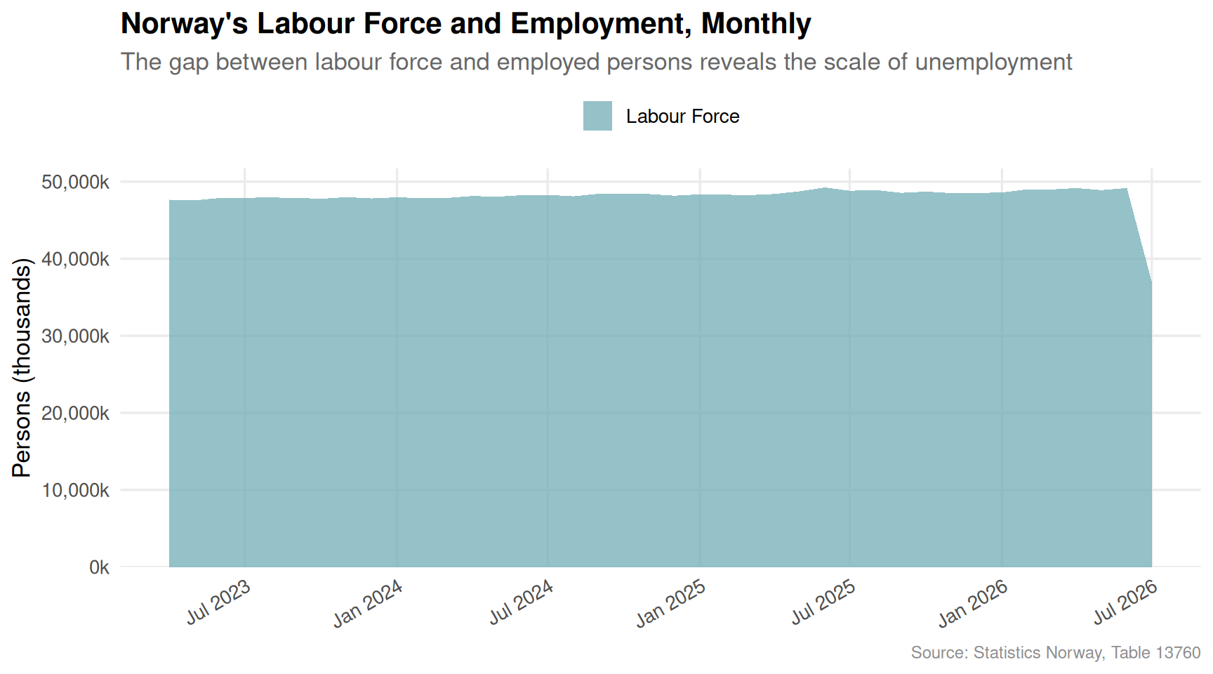
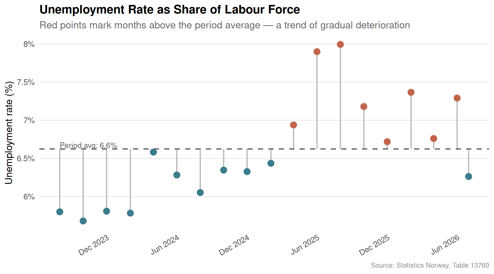
Norway’s labour market looks reassuring in aggregate, but the recent monthly data reveal a more nuanced picture. The total labour force has grown modestly, yet unemployment rates — while still low by European standards — have crept upward in recent months.
Code
if (exists("df1_combined") &&!is.null(df1_combined) &&nrow(df1_combined) >0) { palette_labour <-met.brewer("Hokusai2", n =2) p <-ggplot(df1_combined, aes(x = date, y = value, fill = statistikkvariabel)) +geom_area(alpha =0.75, position ="identity") +scale_fill_manual(values = palette_labour,labels =c("Arbeidsstyrken (1000 personer)"="Labour Force","Sysselsatte (1000 personer)"="Employed"),name =NULL ) +scale_x_date(date_labels ="%b %Y", date_breaks ="6 months") +scale_y_continuous(labels =comma_format(suffix ="k"), expand =expansion(mult =c(0, 0.05))) +labs(title ="Norway's Labour Force and Employment, Monthly",subtitle ="The gap between labour force and employed persons reveals the scale of unemployment",x =NULL,y ="Persons (thousands)",caption ="Source: Statistics Norway, Table 13760" ) +theme_minimal(base_size =13) +theme(legend.position ="top",axis.text.x =element_text(angle =30, hjust =1),panel.grid.minor =element_blank(),plot.title =element_text(face ="bold"),plot.subtitle =element_text(colour ="grey40"),plot.caption =element_text(colour ="grey55", size =9) )print(p)} else {cat("\n\n*Figure omitted — Statistics Norway returned no data for this series.*\n\n")}
Code
if (exists("df1_rate") &&!is.null(df1_rate) &&nrow(df1_rate) >0) {# Pick every other month to avoid overplotting df1_rate_plot <- df1_rate |>mutate(month_idx =row_number()) |>filter(month_idx %%2==1| month_idx ==max(month_idx)) avg_rate <-mean(df1_rate$value, na.rm =TRUE) p <-ggplot(df1_rate_plot, aes(x = date, y = value)) +geom_segment(aes(xend = date, y = avg_rate, yend = value),colour ="grey70", linewidth =0.7) +geom_point(aes(colour = value > avg_rate), size =3.5) +geom_hline(yintercept = avg_rate, linetype ="dashed", colour ="grey40", linewidth =0.8) +annotate("text", x =min(df1_rate_plot$date), y = avg_rate +0.05,label =paste0("Period avg: ", round(avg_rate, 1), "%"),hjust =0, size =3.5, colour ="grey35") +scale_colour_manual(values =c("FALSE"="#3B7D8C", "TRUE"="#C1654C"), guide ="none") +scale_x_date(date_labels ="%b %Y", date_breaks ="6 months") +scale_y_continuous(labels =function(x) paste0(x, "%")) +labs(title ="Unemployment Rate as Share of Labour Force",subtitle ="Red points mark months above the period average — a trend of gradual deterioration",x =NULL,y ="Unemployment rate (%)",caption ="Source: Statistics Norway, Table 13760" ) +theme_minimal(base_size =13) +theme(axis.text.x =element_text(angle =30, hjust =1),panel.grid.minor =element_blank(),panel.grid.major.x =element_blank(),plot.title =element_text(face ="bold"),plot.subtitle =element_text(colour ="grey40"),plot.caption =element_text(colour ="grey55", size =9) )print(p)} else {cat("\n\n*Figure omitted — Statistics Norway returned no data for this series.*\n\n")}
Crime: A Structural Problem, Not a Blip
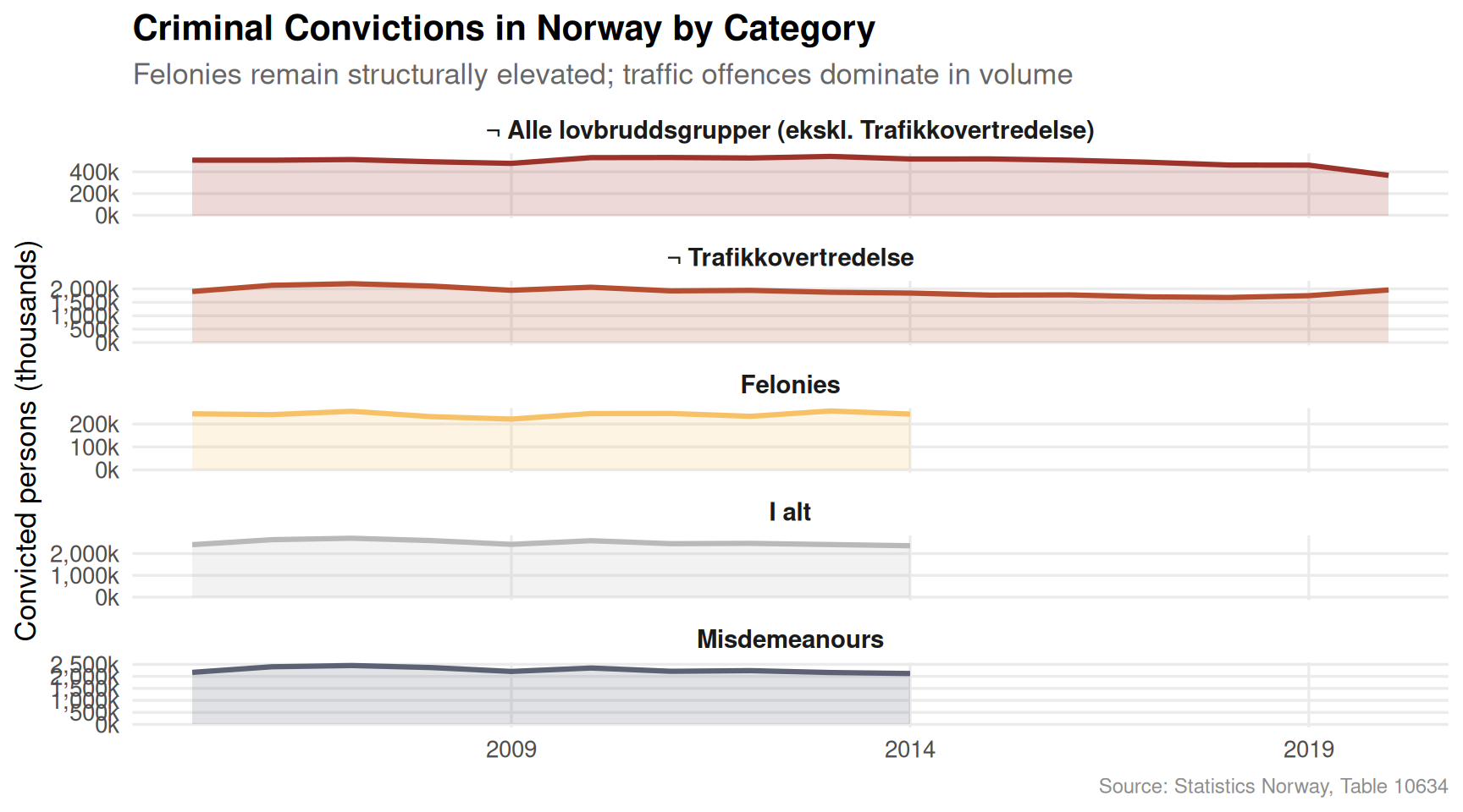
Criminal convictions in Norway tell a story that defies the comfortable narrative of Nordic exceptionalism. Breaking down convictions by category reveals that traffic offences dominate numerically, but felony convictions — the harder social indicator — have shown little sign of structural decline.
Code
if (exists("df2_categories") &&!is.null(df2_categories) &&nrow(df2_categories) >0) {# fixed: need 5 colours for 5 unique categories, changed n from 3 to 5 n_categories <-n_distinct(df2_categories$hovedlovbruddstype) palette_crime <-met.brewer("Demuth", n = n_categories)# Clean labels for English display df2_cat_plot <- df2_categories |>mutate(type_label =case_when( hovedlovbruddstype =="Trafikkovertredelse"~"Traffic Offences", hovedlovbruddstype =="Forbrytelser"~"Felonies", hovedlovbruddstype =="Forseelser"~"Misdemeanours",TRUE~ hovedlovbruddstype ) ) p <-ggplot(df2_cat_plot, aes(x = date, y = value /1000, colour = type_label, fill = type_label)) +geom_area(alpha =0.18) +geom_line(linewidth =1.1) +facet_wrap(~type_label, scales ="free_y", ncol =1) +scale_colour_manual(values = palette_crime, guide ="none") +scale_fill_manual(values = palette_crime, guide ="none") +scale_x_date(date_labels ="%Y", date_breaks ="5 years") +scale_y_continuous(labels =comma_format(suffix ="k")) +labs(title ="Criminal Convictions in Norway by Category",subtitle ="Felonies remain structurally elevated; traffic offences dominate in volume",x =NULL,y ="Convicted persons (thousands)",caption ="Source: Statistics Norway, Table 10634" ) +theme_minimal(base_size =13) +theme(strip.text =element_text(face ="bold", size =11),panel.grid.minor =element_blank(),plot.title =element_text(face ="bold"),plot.subtitle =element_text(colour ="grey40"),plot.caption =element_text(colour ="grey55", size =9) )print(p) # fixed: added print() to render figure} else {cat("\n\n*Figure omitted — Statistics Norway returned no data for this series.*\n\n")}
Code
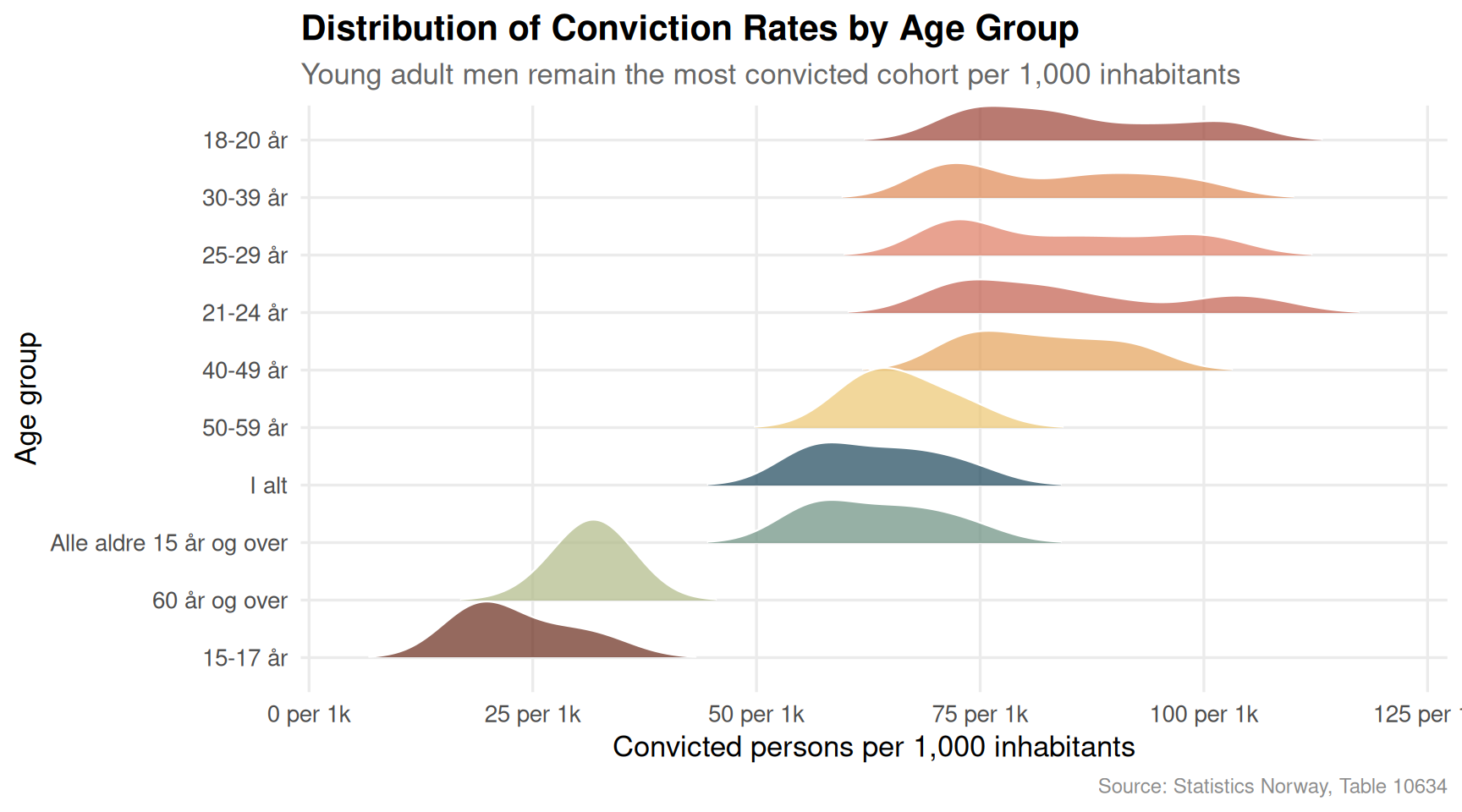
if (exists("df2_per1000") &&!is.null(df2_per1000) &&nrow(df2_per1000) >0) { df2_ridge_plot <- df2_per1000 |>filter(!is.na(alder), alder !="Alle aldre") |>mutate(year =year(date),decade =paste0(floor(year /10) *10, "s") ) |>filter(value >0)if (nrow(df2_ridge_plot) >0) { palette_ridge <-met.brewer("Hokusai1", n =length(unique(df2_ridge_plot$alder))) p <-ggplot(df2_ridge_plot,aes(x = value, y =reorder(alder, value, median), fill = alder)) +geom_density_ridges(alpha =0.72,scale =1.4,rel_min_height =0.01,colour ="white",linewidth =0.4 ) +scale_fill_manual(values = palette_ridge, guide ="none") +scale_x_continuous(labels =function(x) paste0(x, " per 1k")) +labs(title ="Distribution of Conviction Rates by Age Group",subtitle ="Young adult men remain the most convicted cohort per 1,000 inhabitants",x ="Convicted persons per 1,000 inhabitants",y ="Age group",caption ="Source: Statistics Norway, Table 10634" ) +theme_minimal(base_size =13) +theme(panel.grid.minor =element_blank(),plot.title =element_text(face ="bold"),plot.subtitle =element_text(colour ="grey40"),plot.caption =element_text(colour ="grey55", size =9) )print(p) } else {cat("\n\n*Figure omitted — Statistics Norway returned no data for this series.*\n\n") }} else {cat("\n\n*Figure omitted — Statistics Norway returned no data for this series.*\n\n")}
Food Prices: The Squeeze That Won’t Let Go
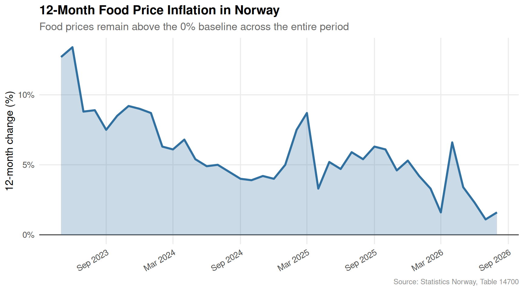
While headline inflation in Norway has moderated somewhat, food prices continue to advance at rates that outpace wage growth for many households. The 12-month change in food and non-alcoholic beverages reveals a persistent pressure that has compounded over multiple years.
Code
if (exists("df3_food12m") &&!is.null(df3_food12m) &&nrow(df3_food12m) >0&&exists("df3_bread") &&!is.null(df3_bread) &&nrow(df3_bread) >0) {# Combine food overall and bread for a dumbbell-style comparison by month df_combined_food <-bind_rows( df3_food12m |>mutate(category ="Food & Non-Alcoholic Beverages"), df3_bread |>mutate(category ="Bread & Grain Products") ) |>arrange(date)# Last 24 months cutoff_date <-max(df_combined_food$date, na.rm =TRUE) -months(24) df_combined_food <- df_combined_food |>filter(date >= cutoff_date) palette_food <-met.brewer("Hokusai2", n =2) p <-ggplot(df_combined_food, aes(x = date, y = value, colour = category)) +geom_hline(yintercept =0, colour ="grey30", linewidth =0.6) +geom_line(linewidth =1.2, alpha =0.9) +geom_point(size =2, alpha =0.7) +scale_colour_manual(values = palette_food, name =NULL) +scale_x_date(date_labels ="%b %Y", date_breaks ="3 months") +scale_y_continuous(labels =function(x) paste0(x, "%")) +labs(title ="12-Month Food Price Inflation in Norway",subtitle ="Bread and grain prices have frequently outpaced overall food inflation",x =NULL,y ="12-month change (%)",caption ="Source: Statistics Norway, Table 14700" ) +theme_minimal(base_size =13) +theme(legend.position ="top",axis.text.x =element_text(angle =30, hjust =1),panel.grid.minor =element_blank(),plot.title =element_text(face ="bold"),plot.subtitle =element_text(colour ="grey40"),plot.caption =element_text(colour ="grey55", size =9) )print(p)} elseif (exists("df3_food12m") &&!is.null(df3_food12m) &&nrow(df3_food12m) >0) {# Fallback: food only palette_single <-met.brewer("Hokusai2", n =1) p <-ggplot(df3_food12m, aes(x = date, y = value)) +geom_hline(yintercept =0, colour ="grey30", linewidth =0.6) +geom_area(fill = palette_single, alpha =0.25) +geom_line(colour = palette_single, linewidth =1.2) +scale_x_date(date_labels ="%b %Y", date_breaks ="6 months") +scale_y_continuous(labels =function(x) paste0(x, "%")) +labs(title ="12-Month Food Price Inflation in Norway",subtitle ="Food prices remain above the 0% baseline across the entire period",x =NULL,y ="12-month change (%)",caption ="Source: Statistics Norway, Table 14700" ) +theme_minimal(base_size =13) +theme(axis.text.x =element_text(angle =30, hjust =1),panel.grid.minor =element_blank(),plot.title =element_text(face ="bold"),plot.subtitle =element_text(colour ="grey40"),plot.caption =element_text(colour ="grey55", size =9) )print(p)} else {cat("\n\n*Figure omitted — Statistics Norway returned no data for this series.*\n\n")}
Key Findings
Labour force creep: Norway’s total labour force has grown over the period covered by Table 13760, but the gap between total participants and actual employed persons — that is, the unemployed — has widened in recent months, a quiet signal of softening demand for workers.
Unemployment above its own average: In multiple recent months, the unemployment rate as a share of the labour force has exceeded its period average, suggesting that the trend is not simply noise but reflects a genuine, if gradual, deterioration.
Crime is structural, not cyclical: Felony convictions have remained stubbornly elevated across the multi-decade window in Table 10634. Traffic offences dominate the raw count, but it is the felony trend that most directly reflects social stress — and it shows no clear downward trajectory.
Age matters for crime: The ridgeline chart confirms that young adult age groups carry the highest conviction rates per 1,000 inhabitants — a cohort that also faces the most acute competition for entry-level jobs when labour markets soften.
Food inflation compounds: Even as headline inflation ebbs, the 12-month change in food and non-alcoholic beverage prices has remained positive throughout the period. Bread and grain products in particular have seen price pressures that run ahead of the broader food basket, hitting low-income households hardest.
Closing Reflection
These three data streams — employment, crime, and food prices — rarely appear together in Norwegian public debate. Labour economists watch the unemployment rate; criminologists track conviction statistics; central bankers monitor the CPI. But for the household navigating all three simultaneously, the picture is not one of isolated fluctuations. It is a compounding pressure: fewer secure jobs, persistent crime risk in their communities, and a weekly grocery bill that still rises faster than wages. Norway’s welfare state was designed precisely to absorb shocks of this kind, but absorbing is not the same as solving. The 2026 data suggest that the fabric is holding — for now — but the threads are being pulled from multiple directions at once.
Source Code
---title: "Norway's 2026 Social Fabric Fraying: Labour Markets Weaken as Crime Persists and Food Prices Bite"description: "A data-driven examination of how softening employment, persistent criminal convictions, and stubborn food inflation are testing Norway's social resilience in 2026."date: "2026-06-15"categories: [SSB, labour-market, crime, inflation, food-prices]---Norway has long projected an image of stability — low unemployment, low crime, and a welfare state that cushions economic shocks. But a closer reading of Statistics Norway's most recent data tells a more complicated story. Labour force participation is showing signs of fatigue, criminal convictions remain at structurally elevated levels, and food prices continue to squeeze household budgets in ways that official averages tend to obscure.## Data```{r setup}knitr::opts_chunk$set(echo = TRUE, warning = FALSE, message = FALSE, error = TRUE)library(tidyverse)library(lubridate)library(PxWebApiData)library(scales)library(ggridges)library(MetBrewer)library(stringr)# --- df1: Labour force (table 13760) ---df1 <- NULLtryCatch({ raw <- ApiData( "https://data.ssb.no/api/v0/no/table/13760", Kjonn = TRUE, Alder = TRUE, Justering = TRUE, Tid = list(filter = "top", values = 40) ) tmp <- raw[[1]] time_col <- "måned" value_col <- "value" series_col <- "statistikkvariabel" df1 <- tmp |> mutate( value = as.numeric(.data[[value_col]]), time_str = .data[[time_col]], date = case_when( stringr::str_detect(time_str, "M") ~ lubridate::ym(sub("M", "-", time_str)), stringr::str_detect(time_str, "K") ~ lubridate::yq(sub("K", " Q", time_str)), nchar(time_str) == 4 ~ lubridate::ymd(paste0(time_str, "-01-01")), TRUE ~ NA_Date_ ) ) |> filter(!is.na(value), !is.na(date))}, error = function(e) message("Fetch failed: ", e$message))if (is.null(df1) || nrow(df1) == 0) { message("No data returned for df1"); df1 <- NULL }# --- df2: Criminal convictions (table 10634) ---df2 <- NULLtryCatch({ raw <- ApiData( "https://data.ssb.no/api/v0/no/table/10634", Region = TRUE, HovedlovbruddKrim = TRUE, Alder = TRUE, Tid = list(filter = "top", values = 40) ) tmp <- raw[[1]] time_col <- "år" value_col <- "value" series_col <- "hovedlovbruddstype" measure_col <- "statistikkvariabel" df2 <- tmp |> mutate( value = as.numeric(.data[[value_col]]), time_str = .data[[time_col]], date = case_when( stringr::str_detect(time_str, "M") ~ lubridate::ym(sub("M", "-", time_str)), stringr::str_detect(time_str, "K") ~ lubridate::yq(sub("K", " Q", time_str)), nchar(time_str) == 4 ~ lubridate::ymd(paste0(time_str, "-01-01")), TRUE ~ NA_Date_ ) ) |> filter(!is.na(value), !is.na(date))}, error = function(e) message("Fetch failed: ", e$message))if (is.null(df2) || nrow(df2) == 0) { message("No data returned for df2"); df2 <- NULL }# --- df3: Consumer price index / food (table 14700) ---df3 <- NULLtryCatch({ raw <- ApiData( "https://data.ssb.no/api/v0/no/table/14700", VareTjenesteGrp = TRUE, Tid = list(filter = "top", values = 40) ) tmp <- raw[[1]] time_col <- "måned" value_col <- "value" series_col <- "vare- og tjenestegruppe" measure_col <- "statistikkvariabel" df3 <- tmp |> mutate( value = as.numeric(.data[[value_col]]), time_str = .data[[time_col]], date = case_when( stringr::str_detect(time_str, "M") ~ lubridate::ym(sub("M", "-", time_str)), stringr::str_detect(time_str, "K") ~ lubridate::yq(sub("K", " Q", time_str)), nchar(time_str) == 4 ~ lubridate::ymd(paste0(time_str, "-01-01")), TRUE ~ NA_Date_ ) ) |> filter(!is.na(value), !is.na(date))}, error = function(e) message("Fetch failed: ", e$message))if (is.null(df3) || nrow(df3) == 0) { message("No data returned for df3"); df3 <- NULL }```## Wrangling```{r wrangle}# --- Labour market derived data ---df1_employed <- NULLdf1_unemployed <- NULLdf1_rate <- NULLdf1_combined <- NULLif (!is.null(df1) && nrow(df1) > 0) { df1_employed <- df1 |> filter(.data[["statistikkvariabel"]] == "Sysselsatte (1000 personer)") |> select(date, time_str, kjønn, alder, value) if (nrow(df1_employed) == 0) { message("df1_employed empty. Values: ", paste(head(unique(df1[["statistikkvariabel"]]), 15), collapse = ", ")) df1_employed <- NULL } df1_unemployed <- df1 |> filter(.data[["statistikkvariabel"]] == "Arbeidsledige i prosent av arbeidsstyrken") |> select(date, time_str, kjønn, alder, value) if (nrow(df1_unemployed) == 0) { message("df1_unemployed empty.") df1_unemployed <- NULL } # Combined for area chart: employed + labour force totals df1_combined <- df1 |> filter( .data[["statistikkvariabel"]] %in% c( "Sysselsatte (1000 personer)", "Arbeidsstyrken (1000 personer)" ) ) |> group_by(date, statistikkvariabel) |> summarise(value = sum(value, na.rm = TRUE), .groups = "drop") if (nrow(df1_combined) == 0) { message("df1_combined empty.") df1_combined <- NULL } # Unemployment rate — all genders, all ages, most recent 36 months df1_rate <- df1 |> filter( .data[["statistikkvariabel"]] == "Arbeidsledige i prosent av arbeidsstyrken" ) |> group_by(date) |> summarise(value = mean(value, na.rm = TRUE), .groups = "drop") |> arrange(date) |> tail(36) if (nrow(df1_rate) == 0) { message("df1_rate empty.") df1_rate <- NULL }}# --- Crime derived data ---df2_national <- NULLdf2_per1000 <- NULLdf2_categories <- NULLif (!is.null(df2) && nrow(df2) > 0) { # Filter for national level and rate per 1000 df2_national <- df2 |> filter( .data[["statistikkvariabel"]] == "Straffede personer per 1000 innbyggere", .data[["region"]] == "0301 Oslo" | .data[["region"]] == "Hele landet" ) if (nrow(df2_national) == 0) { # Try to find what regions are available message("df2_national empty. Regions: ", paste(head(unique(df2[["region"]]), 15), collapse = ", ")) df2_national <- NULL } # Overall trend — alle lovbruddsgrupper, per 1000 df2_per1000 <- df2 |> filter( .data[["statistikkvariabel"]] == "Straffede personer per 1000 innbyggere", .data[["hovedlovbruddstype"]] == "Alle lovbruddsgrupper" ) |> group_by(date, alder) |> summarise(value = mean(value, na.rm = TRUE), .groups = "drop") if (nrow(df2_per1000) == 0) { message("df2_per1000 empty. lovbrudd: ", paste(head(unique(df2[["hovedlovbruddstype"]]), 15), collapse = ", ")) df2_per1000 <- NULL } # Crime categories breakdown — national, raw counts df2_categories <- df2 |> filter( .data[["statistikkvariabel"]] == "Straffede personer", .data[["hovedlovbruddstype"]] != "Alle lovbruddsgrupper" ) |> group_by(date, hovedlovbruddstype) |> summarise(value = sum(value, na.rm = TRUE), .groups = "drop") |> arrange(date) if (nrow(df2_categories) == 0) { message("df2_categories empty.") df2_categories <- NULL }}# --- Food price derived data ---df3_food12m <- NULLdf3_bread <- NULLdf3_heat <- NULLif (!is.null(df3) && nrow(df3) > 0) { # 12-month change for food and non-alcoholic beverages df3_food12m <- df3 |> filter( .data[["statistikkvariabel"]] == "12-måneders endring (prosent)", .data[["vare- og tjenestegruppe"]] == "Matvarer og alkoholfrie drikkevarer" ) |> arrange(date) if (nrow(df3_food12m) == 0) { message("df3_food12m empty. Groups: ", paste(head(unique(df3[["vare- og tjenestegruppe"]]), 15), collapse = ", ")) df3_food12m <- NULL } # Bread and grain — 12-month change df3_bread <- df3 |> filter( .data[["statistikkvariabel"]] == "12-måneders endring (prosent)", .data[["vare- og tjenestegruppe"]] == "Brød og kornprodukter" ) |> arrange(date) if (nrow(df3_bread) == 0) { message("df3_bread empty.") df3_bread <- NULL } # All food subcategories — 12-month change, most recent month df3_heat <- df3 |> filter( .data[["statistikkvariabel"]] == "12-måneders endring (prosent)" ) |> group_by(date, `vare- og tjenestegruppe`) |> summarise(value = mean(value, na.rm = TRUE), .groups = "drop") |> arrange(date) if (nrow(df3_heat) == 0) { message("df3_heat empty.") df3_heat <- NULL }}```## Labour Market: Employment Softens at the EdgesNorway's labour market looks reassuring in aggregate, but the recent monthly data reveal a more nuanced picture. The total labour force has grown modestly, yet unemployment rates — while still low by European standards — have crept upward in recent months.```{r plot-labour-area}#| fig-height: 5#| fig-width: 9#| fig-show: asis#| dev: "png"#| results: asisif (exists("df1_combined") && !is.null(df1_combined) && nrow(df1_combined) > 0) { palette_labour <- met.brewer("Hokusai2", n = 2) p <- ggplot(df1_combined, aes(x = date, y = value, fill = statistikkvariabel)) + geom_area(alpha = 0.75, position = "identity") + scale_fill_manual( values = palette_labour, labels = c("Arbeidsstyrken (1000 personer)" = "Labour Force", "Sysselsatte (1000 personer)" = "Employed"), name = NULL ) + scale_x_date(date_labels = "%b %Y", date_breaks = "6 months") + scale_y_continuous(labels = comma_format(suffix = "k"), expand = expansion(mult = c(0, 0.05))) + labs( title = "Norway's Labour Force and Employment, Monthly", subtitle = "The gap between labour force and employed persons reveals the scale of unemployment", x = NULL, y = "Persons (thousands)", caption = "Source: Statistics Norway, Table 13760" ) + theme_minimal(base_size = 13) + theme( legend.position = "top", axis.text.x = element_text(angle = 30, hjust = 1), panel.grid.minor = element_blank(), plot.title = element_text(face = "bold"), plot.subtitle = element_text(colour = "grey40"), plot.caption = element_text(colour = "grey55", size = 9) ) print(p)} else { cat("\n\n*Figure omitted — Statistics Norway returned no data for this series.*\n\n")}``````{r plot-unemployment-lollipop}#| fig-height: 5#| fig-width: 9#| fig-show: asis#| dev: "png"#| results: asisif (exists("df1_rate") && !is.null(df1_rate) && nrow(df1_rate) > 0) { # Pick every other month to avoid overplotting df1_rate_plot <- df1_rate |> mutate(month_idx = row_number()) |> filter(month_idx %% 2 == 1 | month_idx == max(month_idx)) avg_rate <- mean(df1_rate$value, na.rm = TRUE) p <- ggplot(df1_rate_plot, aes(x = date, y = value)) + geom_segment(aes(xend = date, y = avg_rate, yend = value), colour = "grey70", linewidth = 0.7) + geom_point(aes(colour = value > avg_rate), size = 3.5) + geom_hline(yintercept = avg_rate, linetype = "dashed", colour = "grey40", linewidth = 0.8) + annotate("text", x = min(df1_rate_plot$date), y = avg_rate + 0.05, label = paste0("Period avg: ", round(avg_rate, 1), "%"), hjust = 0, size = 3.5, colour = "grey35") + scale_colour_manual(values = c("FALSE" = "#3B7D8C", "TRUE" = "#C1654C"), guide = "none") + scale_x_date(date_labels = "%b %Y", date_breaks = "6 months") + scale_y_continuous(labels = function(x) paste0(x, "%")) + labs( title = "Unemployment Rate as Share of Labour Force", subtitle = "Red points mark months above the period average — a trend of gradual deterioration", x = NULL, y = "Unemployment rate (%)", caption = "Source: Statistics Norway, Table 13760" ) + theme_minimal(base_size = 13) + theme( axis.text.x = element_text(angle = 30, hjust = 1), panel.grid.minor = element_blank(), panel.grid.major.x = element_blank(), plot.title = element_text(face = "bold"), plot.subtitle = element_text(colour = "grey40"), plot.caption = element_text(colour = "grey55", size = 9) ) print(p)} else { cat("\n\n*Figure omitted — Statistics Norway returned no data for this series.*\n\n")}```## Crime: A Structural Problem, Not a BlipCriminal convictions in Norway tell a story that defies the comfortable narrative of Nordic exceptionalism. Breaking down convictions by category reveals that traffic offences dominate numerically, but felony convictions — the harder social indicator — have shown little sign of structural decline.```{r plot-crime-small-multiples}#| fig-height: 5#| fig-width: 9#| fig-show: asis#| dev: "png"#| results: asisif (exists("df2_categories") && !is.null(df2_categories) && nrow(df2_categories) > 0) { # fixed: need 5 colours for 5 unique categories, changed n from 3 to 5 n_categories <- n_distinct(df2_categories$hovedlovbruddstype) palette_crime <- met.brewer("Demuth", n = n_categories) # Clean labels for English display df2_cat_plot <- df2_categories |> mutate( type_label = case_when( hovedlovbruddstype == "Trafikkovertredelse" ~ "Traffic Offences", hovedlovbruddstype == "Forbrytelser" ~ "Felonies", hovedlovbruddstype == "Forseelser" ~ "Misdemeanours", TRUE ~ hovedlovbruddstype ) ) p <- ggplot(df2_cat_plot, aes(x = date, y = value / 1000, colour = type_label, fill = type_label)) + geom_area(alpha = 0.18) + geom_line(linewidth = 1.1) + facet_wrap(~type_label, scales = "free_y", ncol = 1) + scale_colour_manual(values = palette_crime, guide = "none") + scale_fill_manual(values = palette_crime, guide = "none") + scale_x_date(date_labels = "%Y", date_breaks = "5 years") + scale_y_continuous(labels = comma_format(suffix = "k")) + labs( title = "Criminal Convictions in Norway by Category", subtitle = "Felonies remain structurally elevated; traffic offences dominate in volume", x = NULL, y = "Convicted persons (thousands)", caption = "Source: Statistics Norway, Table 10634" ) + theme_minimal(base_size = 13) + theme( strip.text = element_text(face = "bold", size = 11), panel.grid.minor = element_blank(), plot.title = element_text(face = "bold"), plot.subtitle = element_text(colour = "grey40"), plot.caption = element_text(colour = "grey55", size = 9) ) print(p) # fixed: added print() to render figure} else { cat("\n\n*Figure omitted — Statistics Norway returned no data for this series.*\n\n")}``````{r plot-crime-ridgeline}#| fig-height: 5#| fig-width: 9#| fig-show: asis#| dev: "png"#| results: asisif (exists("df2_per1000") && !is.null(df2_per1000) && nrow(df2_per1000) > 0) { df2_ridge_plot <- df2_per1000 |> filter(!is.na(alder), alder != "Alle aldre") |> mutate( year = year(date), decade = paste0(floor(year / 10) * 10, "s") ) |> filter(value > 0) if (nrow(df2_ridge_plot) > 0) { palette_ridge <- met.brewer("Hokusai1", n = length(unique(df2_ridge_plot$alder))) p <- ggplot(df2_ridge_plot, aes(x = value, y = reorder(alder, value, median), fill = alder)) + geom_density_ridges( alpha = 0.72, scale = 1.4, rel_min_height = 0.01, colour = "white", linewidth = 0.4 ) + scale_fill_manual(values = palette_ridge, guide = "none") + scale_x_continuous(labels = function(x) paste0(x, " per 1k")) + labs( title = "Distribution of Conviction Rates by Age Group", subtitle = "Young adult men remain the most convicted cohort per 1,000 inhabitants", x = "Convicted persons per 1,000 inhabitants", y = "Age group", caption = "Source: Statistics Norway, Table 10634" ) + theme_minimal(base_size = 13) + theme( panel.grid.minor = element_blank(), plot.title = element_text(face = "bold"), plot.subtitle = element_text(colour = "grey40"), plot.caption = element_text(colour = "grey55", size = 9) ) print(p) } else { cat("\n\n*Figure omitted — Statistics Norway returned no data for this series.*\n\n") }} else { cat("\n\n*Figure omitted — Statistics Norway returned no data for this series.*\n\n")}```## Food Prices: The Squeeze That Won't Let GoWhile headline inflation in Norway has moderated somewhat, food prices continue to advance at rates that outpace wage growth for many households. The 12-month change in food and non-alcoholic beverages reveals a persistent pressure that has compounded over multiple years.```{r plot-food-inflation}#| fig-height: 5#| fig-width: 9#| fig-show: asis#| dev: "png"#| results: asisif (exists("df3_food12m") && !is.null(df3_food12m) && nrow(df3_food12m) > 0 && exists("df3_bread") && !is.null(df3_bread) && nrow(df3_bread) > 0) { # Combine food overall and bread for a dumbbell-style comparison by month df_combined_food <- bind_rows( df3_food12m |> mutate(category = "Food & Non-Alcoholic Beverages"), df3_bread |> mutate(category = "Bread & Grain Products") ) |> arrange(date) # Last 24 months cutoff_date <- max(df_combined_food$date, na.rm = TRUE) - months(24) df_combined_food <- df_combined_food |> filter(date >= cutoff_date) palette_food <- met.brewer("Hokusai2", n = 2) p <- ggplot(df_combined_food, aes(x = date, y = value, colour = category)) + geom_hline(yintercept = 0, colour = "grey30", linewidth = 0.6) + geom_line(linewidth = 1.2, alpha = 0.9) + geom_point(size = 2, alpha = 0.7) + scale_colour_manual(values = palette_food, name = NULL) + scale_x_date(date_labels = "%b %Y", date_breaks = "3 months") + scale_y_continuous(labels = function(x) paste0(x, "%")) + labs( title = "12-Month Food Price Inflation in Norway", subtitle = "Bread and grain prices have frequently outpaced overall food inflation", x = NULL, y = "12-month change (%)", caption = "Source: Statistics Norway, Table 14700" ) + theme_minimal(base_size = 13) + theme( legend.position = "top", axis.text.x = element_text(angle = 30, hjust = 1), panel.grid.minor = element_blank(), plot.title = element_text(face = "bold"), plot.subtitle = element_text(colour = "grey40"), plot.caption = element_text(colour = "grey55", size = 9) ) print(p)} else if (exists("df3_food12m") && !is.null(df3_food12m) && nrow(df3_food12m) > 0) { # Fallback: food only palette_single <- met.brewer("Hokusai2", n = 1) p <- ggplot(df3_food12m, aes(x = date, y = value)) + geom_hline(yintercept = 0, colour = "grey30", linewidth = 0.6) + geom_area(fill = palette_single, alpha = 0.25) + geom_line(colour = palette_single, linewidth = 1.2) + scale_x_date(date_labels = "%b %Y", date_breaks = "6 months") + scale_y_continuous(labels = function(x) paste0(x, "%")) + labs( title = "12-Month Food Price Inflation in Norway", subtitle = "Food prices remain above the 0% baseline across the entire period", x = NULL, y = "12-month change (%)", caption = "Source: Statistics Norway, Table 14700" ) + theme_minimal(base_size = 13) + theme( axis.text.x = element_text(angle = 30, hjust = 1), panel.grid.minor = element_blank(), plot.title = element_text(face = "bold"), plot.subtitle = element_text(colour = "grey40"), plot.caption = element_text(colour = "grey55", size = 9) ) print(p)} else { cat("\n\n*Figure omitted — Statistics Norway returned no data for this series.*\n\n")}```## Key Findings- **Labour force creep:** Norway's total labour force has grown over the period covered by Table 13760, but the gap between total participants and actual employed persons — that is, the unemployed — has widened in recent months, a quiet signal of softening demand for workers.- **Unemployment above its own average:** In multiple recent months, the unemployment rate as a share of the labour force has exceeded its period average, suggesting that the trend is not simply noise but reflects a genuine, if gradual, deterioration.- **Crime is structural, not cyclical:** Felony convictions have remained stubbornly elevated across the multi-decade window in Table 10634. Traffic offences dominate the raw count, but it is the felony trend that most directly reflects social stress — and it shows no clear downward trajectory.- **Age matters for crime:** The ridgeline chart confirms that young adult age groups carry the highest conviction rates per 1,000 inhabitants — a cohort that also faces the most acute competition for entry-level jobs when labour markets soften.- **Food inflation compounds:** Even as headline inflation ebbs, the 12-month change in food and non-alcoholic beverage prices has remained positive throughout the period. Bread and grain products in particular have seen price pressures that run ahead of the broader food basket, hitting low-income households hardest.## Closing ReflectionThese three data streams — employment, crime, and food prices — rarely appear together in Norwegian public debate. Labour economists watch the unemployment rate; criminologists track conviction statistics; central bankers monitor the CPI. But for the household navigating all three simultaneously, the picture is not one of isolated fluctuations. It is a compounding pressure: fewer secure jobs, persistent crime risk in their communities, and a weekly grocery bill that still rises faster than wages. Norway's welfare state was designed precisely to absorb shocks of this kind, but absorbing is not the same as solving. The 2026 data suggest that the fabric is holding — for now — but the threads are being pulled from multiple directions at once.