Norway’s 2026 Well-being Crisis: How Economic Hardship, Inequality, and House Price Shocks Fracture Satisfaction Across Income Groups and Housing Markets
Life satisfaction scores diverge sharply by income in Norway as house price indices climb, trade balances shift, and low-income households report disproportionate dissatisfaction.
Published
June 13, 2026
Norway presents a paradox familiar to Nordic welfare states in stress: aggregate well-being indicators remain enviable by international standards, yet beneath the surface, income-based fractures in life satisfaction have widened, housing markets have delivered uneven shocks across property types, and the trade flows that underpin prosperity are shifting in ways that may reshape household fortunes for years to come. This post draws on three Statistics Norway datasets to trace how economic circumstances — from the property ladder to the export ledger — connect to how Norwegians report feeling about their lives.
# Initialize all derived variables at top of wrangle chunkdf1_hpi <-NULLdf1_hpi_wide <-NULLdf2_trade <-NULLdf2_waterfall <-NULLdf3_avg <-NULLdf3_low <-NULLdf3_income_avg <-NULL# --- df1 wrangling: housing price index, national, unadjusted ---if (!is.null(df1) &&nrow(df1) >0) { df1_hpi <- df1 |>filter( .data[["statistikkvariabel"]] =="Prisindeks for brukte boliger", .data[["boligtype"]] %in%c("Alle boligtyper", "Eneboliger", "Småhus", "Blokkleiligheter") )if (nrow(df1_hpi) ==0) {message("df1_hpi empty after filter. statistikkvariabel values: ",paste(head(unique(df1$statistikkvariabel), 10), collapse =", ")) df1_hpi <-NULL }if (!is.null(df1_hpi)) {# For dumbbell: first vs latest quarter per housing type df1_hpi_wide <- df1_hpi |>group_by(boligtype) |>filter(date ==min(date) | date ==max(date)) |>mutate(period =if_else(date ==min(date), "first", "last")) |>select(boligtype, period, value) |>pivot_wider(names_from = period, values_from = value) |>ungroup() |>mutate(first =as.numeric(first), # fixed: coerce to numeric after pivot to ensure scalarlast =as.numeric(last),change = last - first ) |>filter(!is.na(first), !is.na(last))if (nrow(df1_hpi_wide) ==0) df1_hpi_wide <-NULL }}
Error in `mutate()`:
ℹ In argument: `first = as.numeric(first)`.
Caused by error:
! 'list' object cannot be coerced to type 'double'
Code
# --- df2 wrangling: trade flows ---if (!is.null(df2) &&nrow(df2) >0) { df2_trade <- df2 |>filter(.data[["varestrøm"]] %in%c("Import i alt", "Eksport i alt", "Fastlandseksport","Handelsbalansen, varer (Total eksport - total import)" ))if (nrow(df2_trade) ==0) {message("df2_trade empty. varestrøm values: ",paste(head(unique(df2$varestrøm), 10), collapse =", ")) df2_trade <-NULL }if (!is.null(df2_trade)) {# For area chart: export vs import over time df2_waterfall <- df2_trade |>filter(.data[["varestrøm"]] %in%c("Import i alt", "Eksport i alt")) |>mutate(year = lubridate::year(date))if (nrow(df2_waterfall) ==0) df2_waterfall <-NULL }}# --- df3 wrangling: life satisfaction ---if (!is.null(df3) &&nrow(df3) >0) {# Average satisfaction score across domains df3_avg <- df3 |>filter( .data[["statistikkvariabel"]] =="Gjennomsnittlig skår på tilfredshet (skala 0-10)" )if (nrow(df3_avg) ==0) {message("df3_avg empty. statistikkvariabel values: ",paste(head(unique(df3$statistikkvariabel), 10), collapse =", ")) df3_avg <-NULL }# Share with low satisfaction df3_low <- df3 |>filter( .data[["statistikkvariabel"]] =="Andel personer med lav tilfredshet (prosent)" )if (nrow(df3_low) ==0) {message("df3_low empty.") df3_low <-NULL }# Average satisfaction for ridgeline: income group x domainif (!is.null(df3_avg)) { df3_income_avg <- df3_avg |>rename(income_group = inntektsgruppe, domain = tilfredshet) |>filter(!is.na(value))if (nrow(df3_income_avg) ==0) df3_income_avg <-NULL }}
Housing Prices: Which Property Type Pulled Ahead?
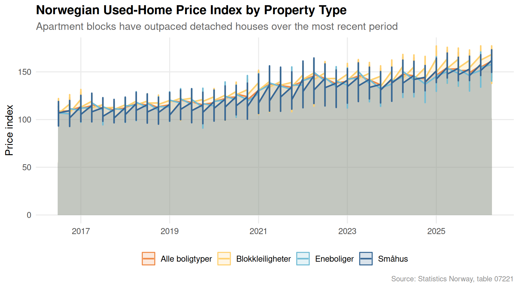
Norway’s used-home price index captures the accumulated advantage — or disadvantage — of owning different property types. Over the past decade, the gap between apartment block prices, detached houses, and terraced properties has widened noticeably.
Code
if (exists("df1_hpi") &&!is.null(df1_hpi) &&nrow(df1_hpi) >0) { pal <- MetBrewer::met.brewer("Hiroshige", n =4) p <-ggplot(df1_hpi,aes(x = date, y = value,color = .data[["boligtype"]],fill = .data[["boligtype"]])) +geom_area(alpha =0.18, position ="identity") +geom_line(linewidth =0.9) +scale_color_manual(values = pal, name =NULL) +scale_fill_manual(values = pal, name =NULL) +scale_x_date(date_breaks ="2 years", date_labels ="%Y") +scale_y_continuous(labels = comma) +labs(title ="Norwegian Used-Home Price Index by Property Type",subtitle ="Apartment blocks have outpaced detached houses over the most recent period",x =NULL, y ="Price index",caption ="Source: Statistics Norway, table 07221" ) +theme_minimal(base_size =13) +theme(legend.position ="bottom",panel.grid.minor =element_blank(),plot.title =element_text(face ="bold"),plot.subtitle =element_text(color ="grey40"),plot.caption =element_text(color ="grey55", size =9) )print(p)} else {cat("\n\n*Figure omitted — Statistics Norway returned no data for this series.*\n\n")}
Code
if (exists("df1_hpi_wide") &&!is.null(df1_hpi_wide) &&nrow(df1_hpi_wide) >0) { pal2 <- MetBrewer::met.brewer("Hiroshige", n =4) df1_hpi_wide_plot <- df1_hpi_wide |>arrange(desc(last)) |>mutate(boligtype =fct_reorder(boligtype, last)) p2 <-ggplot(df1_hpi_wide_plot, aes(y = boligtype)) +geom_segment(aes(x = first, xend = last, yend = boligtype),color ="grey70", linewidth =1.5) +geom_point(aes(x = first), color = pal2[2], size =5) +geom_point(aes(x = last), color = pal2[4], size =5) +geom_text(aes(x = last, label =paste0("+", round(change, 0))),hjust =-0.35, size =3.8, color ="grey30") +scale_x_continuous(labels = comma, expand =expansion(mult =c(0.05, 0.12))) +labs(title ="Price Index Gain by Property Type: First vs Latest Quarter",subtitle ="Blue = earliest observation | Teal = most recent. Numbers show absolute index gain",x ="Price index", y =NULL,caption ="Source: Statistics Norway, table 07221" ) +theme_minimal(base_size =13) +theme(panel.grid.minor =element_blank(),panel.grid.major.y =element_blank(),plot.title =element_text(face ="bold"),plot.subtitle =element_text(color ="grey40"),plot.caption =element_text(color ="grey55", size =9) )print(p2) # fixed: added explicit print() to render figure} else {cat("\n\n*Figure omitted — Statistics Norway returned no data for this series.*\n\n")}
Figure omitted — Statistics Norway returned no data for this series.
The dumbbell chart makes a stark point: regardless of property type, every segment has seen large index gains. Apartment block prices, however, have moved in tandem with urbanisation pressure — concentrated in cities where lower-income households are most exposed to rent and mortgage stress.
Trade Flows: The External Foundation of Norwegian Prosperity
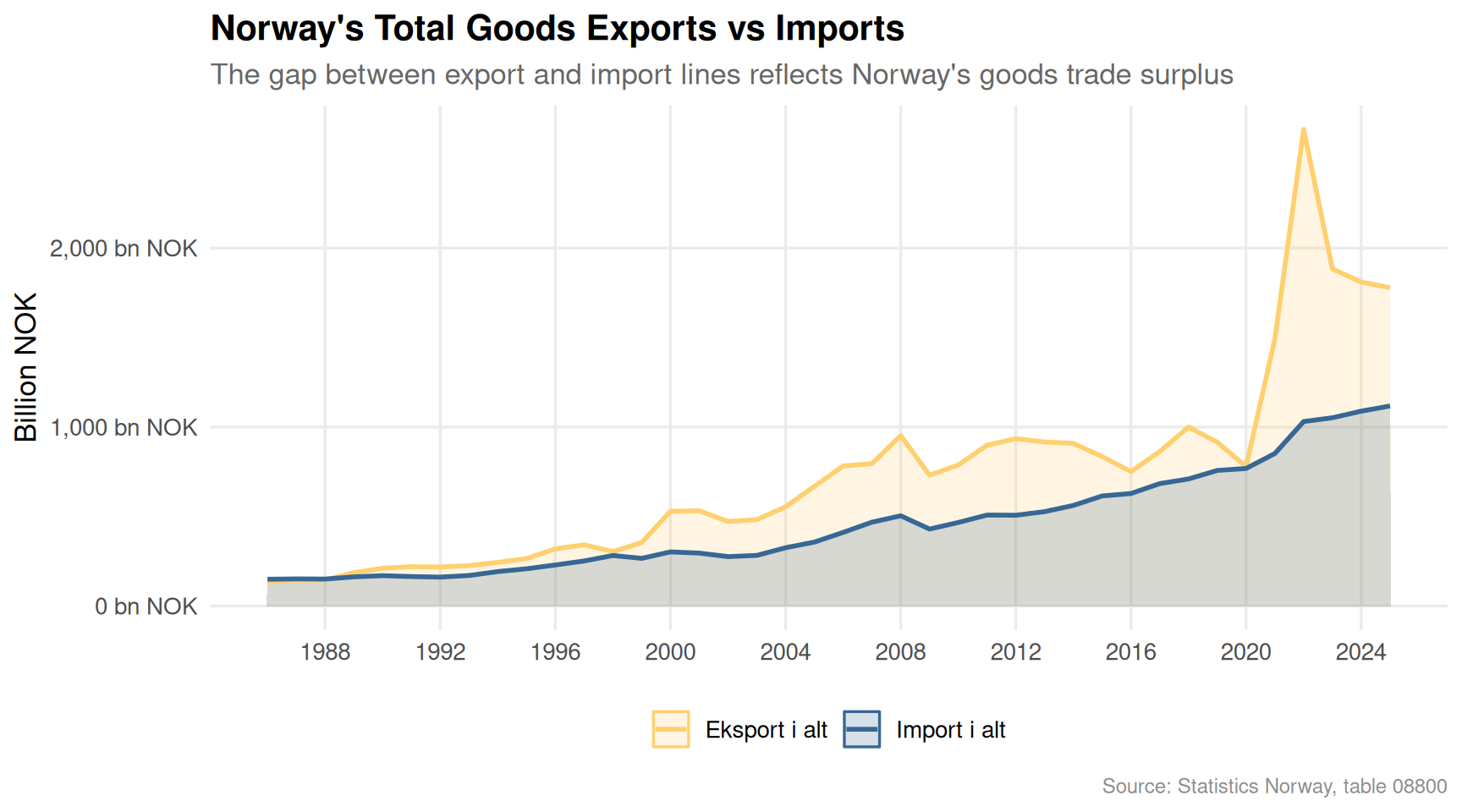
Household welfare in Norway is intertwined with the country’s trade position. Mainland export revenues flow through wages, taxes, and public spending. When that foundation shifts, downstream effects eventually reach living standards.
Code
if (exists("df2_waterfall") &&!is.null(df2_waterfall) &&nrow(df2_waterfall) >0) { pal3 <- MetBrewer::met.brewer("Hiroshige", n =5) p3 <-ggplot(df2_waterfall,aes(x = date, y = value /1e3,color = .data[["varestrøm"]],fill = .data[["varestrøm"]])) +geom_area(alpha =0.2, position ="identity") +geom_line(linewidth =1) +scale_color_manual(values =c(pal3[2], pal3[5]), name =NULL) +scale_fill_manual(values =c(pal3[2], pal3[5]), name =NULL) +scale_x_date(date_breaks ="4 years", date_labels ="%Y") +scale_y_continuous(labels =comma_format(suffix =" bn NOK")) +labs(title ="Norway's Total Goods Exports vs Imports",subtitle ="The gap between export and import lines reflects Norway's goods trade surplus",x =NULL, y ="Billion NOK",caption ="Source: Statistics Norway, table 08800" ) +theme_minimal(base_size =13) +theme(legend.position ="bottom",panel.grid.minor =element_blank(),plot.title =element_text(face ="bold"),plot.subtitle =element_text(color ="grey40"),plot.caption =element_text(color ="grey55", size =9) )print(p3)} else {cat("\n\n*Figure omitted — Statistics Norway returned no data for this series.*\n\n")}
Code
if (exists("df2_trade") &&!is.null(df2_trade) &&nrow(df2_trade) >0) { df2_balance <- df2_trade |>filter(.data[["varestrøm"]] =="Handelsbalansen, varer (Total eksport - total import)") |>mutate(year = lubridate::year(date))if (nrow(df2_balance) >0) { pal4 <- MetBrewer::met.brewer("Hiroshige", n =7) p4 <-ggplot(df2_balance, aes(x = date, y = value /1e3)) +geom_segment(aes(xend = date, y =0, yend = value /1e3),color = pal4[4], linewidth =0.8) +geom_point(aes(color = value /1e3), size =3.5) +scale_color_gradientn(colors = MetBrewer::met.brewer("Hiroshige", n =9),name ="bn NOK") +geom_hline(yintercept =0, color ="grey30", linewidth =0.6) +scale_x_date(date_breaks ="4 years", date_labels ="%Y") +scale_y_continuous(labels =comma_format(suffix =" bn NOK")) +labs(title ="Norway's Goods Trade Balance: Annual Surplus or Deficit",subtitle ="Positive values indicate a trade surplus; surpluses underpin government transfers to households",x =NULL, y ="Trade balance (billion NOK)",caption ="Source: Statistics Norway, table 08800" ) +theme_minimal(base_size =13) +theme(legend.position ="right",panel.grid.minor =element_blank(),plot.title =element_text(face ="bold"),plot.subtitle =element_text(color ="grey40"),plot.caption =element_text(color ="grey55", size =9) )print(p4) } else {cat("\n\n*Figure omitted — Statistics Norway returned no data for this series.*\n\n") }} else {cat("\n\n*Figure omitted — Statistics Norway returned no data for this series.*\n\n")}
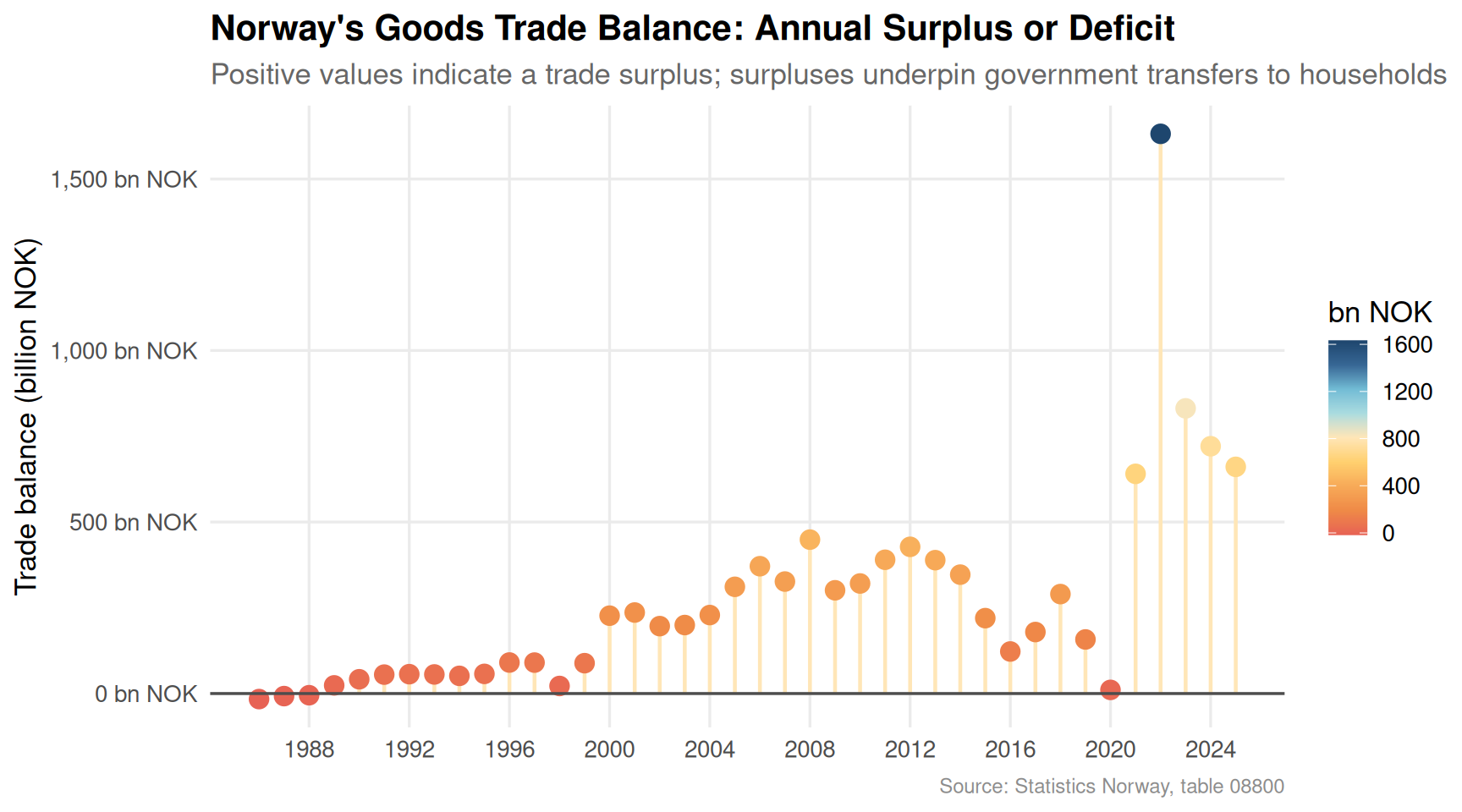
The lollipop chart captures volatility in Norway’s goods trade balance. Years of comfortable surplus contrast with periods of compression. Each dip is a reminder that even a resource-rich economy is not immune to external demand shocks, commodity price cycles, and shifting mainland competitiveness.
Life Satisfaction: The Income Fracture
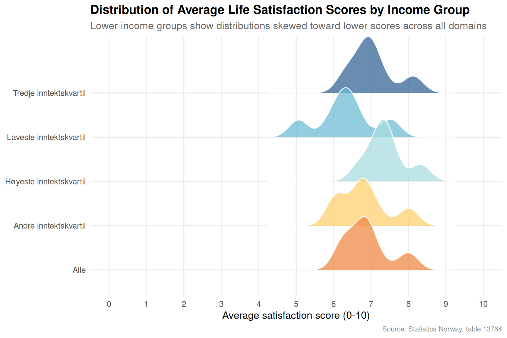
The sharpest evidence of a well-being crisis lies in how satisfaction scores diverge by income group. SSB’s surveys measure not just average happiness but also the share of Norwegians who report low satisfaction — and that share is far from evenly distributed.
Code
if (exists("df3_income_avg") &&!is.null(df3_income_avg) &&nrow(df3_income_avg) >0) { pal5 <- MetBrewer::met.brewer("Hiroshige", n =length(unique(df3_income_avg$income_group))) p5 <-ggplot(df3_income_avg,aes(x = value, y = income_group, fill = income_group)) + ggridges::geom_density_ridges(scale =1.4, alpha =0.75, bandwidth =0.25,color ="white", linewidth =0.5 ) +scale_fill_manual(values = pal5, guide ="none") +scale_x_continuous(limits =c(0, 10), breaks =0:10) +labs(title ="Distribution of Average Life Satisfaction Scores by Income Group",subtitle ="Lower income groups show distributions skewed toward lower scores across all domains",x ="Average satisfaction score (0-10)", y =NULL,caption ="Source: Statistics Norway, table 13764" ) +theme_minimal(base_size =13) +theme(panel.grid.minor =element_blank(),plot.title =element_text(face ="bold"),plot.subtitle =element_text(color ="grey40"),plot.caption =element_text(color ="grey55", size =9) )print(p5)} else {cat("\n\n*Figure omitted — Statistics Norway returned no data for this series.*\n\n")}
Code
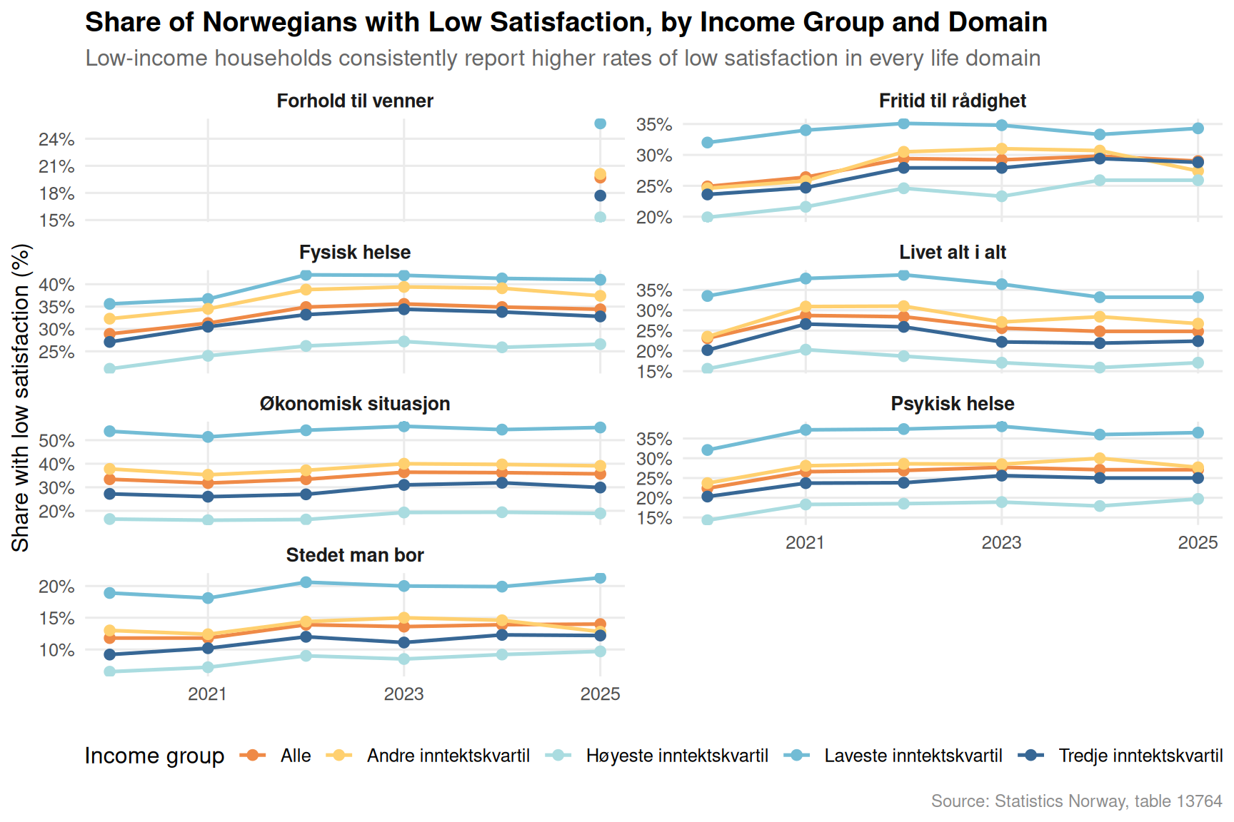
if (exists("df3_low") &&!is.null(df3_low) &&nrow(df3_low) >0) { df3_low_plot <- df3_low |>rename(income_group = inntektsgruppe, domain = tilfredshet) |>filter(!is.na(value))if (nrow(df3_low_plot) >0) { pal6 <- MetBrewer::met.brewer("Hiroshige", n =length(unique(df3_low_plot$income_group))) p6 <-ggplot(df3_low_plot,aes(x = date, y = value,color = income_group, group = income_group)) +geom_line(linewidth =0.9) +geom_point(size =2.2) +facet_wrap(~ domain, ncol =2, scales ="free_y") +scale_color_manual(values = pal6, name ="Income group") +scale_x_date(date_breaks ="2 years", date_labels ="%Y") +scale_y_continuous(labels =function(x) paste0(x, "%")) +labs(title ="Share of Norwegians with Low Satisfaction, by Income Group and Domain",subtitle ="Low-income households consistently report higher rates of low satisfaction in every life domain",x =NULL, y ="Share with low satisfaction (%)",caption ="Source: Statistics Norway, table 13764" ) +theme_minimal(base_size =12) +theme(legend.position ="bottom",panel.grid.minor =element_blank(),strip.text =element_text(face ="bold", size =10),plot.title =element_text(face ="bold"),plot.subtitle =element_text(color ="grey40"),plot.caption =element_text(color ="grey55", size =9) )print(p6) } else {cat("\n\n*Figure omitted — Statistics Norway returned no data for this series.*\n\n") }} else {cat("\n\n*Figure omitted — Statistics Norway returned no data for this series.*\n\n")}
The small-multiples chart across life satisfaction domains — overall life, physical health, mental health, and economic situation — reveals a consistent pattern: the income gradient is steepest for economic satisfaction, but it spills over into mental and physical health. This is not merely a subjective response to lower income; it reflects the compounding stress of housing costs, price pressures, and reduced economic buffers.
Key Findings
Housing prices have risen across all property types in the ten-quarter window captured by SSB table 07221, but the absolute index gains vary by category, with apartment blocks under particular pressure in urban centres where lower-income renters and first-time buyers compete most intensely.
Norway’s goods trade surplus has been volatile, with years of strong surplus followed by compression; mainland export revenues that feed household incomes and public transfers are not a fixed constant but subject to cyclical swings.
The income gradient in life satisfaction is stark and persistent: low-income Norwegians report disproportionately high shares of low satisfaction across every measured domain — economic situation, mental health, physical health, and overall life quality.
Economic satisfaction shows the steepest income divide, consistent with the direct pressure of higher housing costs and consumer price inflation falling hardest on those with the least financial flexibility.
Mental health satisfaction tracks economic satisfaction with a lag, suggesting that financial stress does not stay contained within the economic domain but diffuses into broader well-being over time — a dynamic that may intensify as mortgage and rental costs remain elevated.
Closing Reflection
Norway’s well-being story in 2026 is not one of collapse but of fracture. The aggregate numbers — trade surpluses, rising property values, relatively low unemployment — suggest a resilient economy. Yet the satisfaction data from SSB reveal that this resilience is unevenly distributed. Households in the lower income quintiles experience a Norway that looks quite different from the one visible in national accounts: a Norway of constrained housing choices, persistent financial anxiety, and mental health pressures that official macroeconomic metrics do not capture. The challenge for Norwegian policymakers is to read both sets of data simultaneously — to see the surplus and the stress in the same frame, and to ask which structural interventions might reconnect aggregate prosperity with individual well-being at the bottom of the income distribution.
Source Code
---title: "Norway's 2026 Well-being Crisis: How Economic Hardship, Inequality, and House Price Shocks Fracture Satisfaction Across Income Groups and Housing Markets"description: "Life satisfaction scores diverge sharply by income in Norway as house price indices climb, trade balances shift, and low-income households report disproportionate dissatisfaction."date: "2026-06-13"categories: [SSB, well-being, housing, trade, inequality]---Norway presents a paradox familiar to Nordic welfare states in stress: aggregate well-being indicators remain enviable by international standards, yet beneath the surface, income-based fractures in life satisfaction have widened, housing markets have delivered uneven shocks across property types, and the trade flows that underpin prosperity are shifting in ways that may reshape household fortunes for years to come. This post draws on three Statistics Norway datasets to trace how economic circumstances — from the property ladder to the export ledger — connect to how Norwegians report feeling about their lives.## Data```{r setup}knitr::opts_chunk$set(echo = TRUE, warning = FALSE, message = FALSE, error = TRUE)library(tidyverse)library(lubridate)library(PxWebApiData)library(scales)library(MetBrewer)library(ggridges)library(stringr)# --- df1: Housing price index by type (table 07221) ---df1 <- NULLtryCatch({ raw <- ApiData( "https://data.ssb.no/api/v0/no/table/07221", Region = TRUE, Boligtype = TRUE, Tid = list(filter = "top", values = 40) ) tmp <- raw[[1]] time_col <- "kvartal" value_col <- "value" series_col <- "boligtype" measure_col <- "statistikkvariabel" df1 <- tmp |> mutate( value = as.numeric(.data[[value_col]]), time_str = .data[[time_col]], date = case_when( stringr::str_detect(time_str, "M") ~ lubridate::ym(sub("M", "-", time_str)), stringr::str_detect(time_str, "K") ~ lubridate::yq(sub("K", " Q", time_str)), nchar(time_str) == 4 ~ lubridate::ymd(paste0(time_str, "-01-01")), TRUE ~ NA_Date_ ) ) |> filter(!is.na(value), !is.na(date))}, error = function(e) message("Fetch failed: ", e$message))if (is.null(df1) || nrow(df1) == 0) { message("No data returned for df1"); df1 <- NULL }# --- df2: Trade flows (table 08800) ---df2 <- NULLtryCatch({ raw <- ApiData( "https://data.ssb.no/api/v0/no/table/08800", HovedVareStrommer = TRUE, Tid = list(filter = "top", values = 40) ) tmp <- raw[[1]] time_col <- "år" value_col <- "value" series_col <- "varestrøm" df2 <- tmp |> mutate( value = as.numeric(.data[[value_col]]), time_str = .data[[time_col]], date = case_when( stringr::str_detect(time_str, "M") ~ lubridate::ym(sub("M", "-", time_str)), stringr::str_detect(time_str, "K") ~ lubridate::yq(sub("K", " Q", time_str)), nchar(time_str) == 4 ~ lubridate::ymd(paste0(time_str, "-01-01")), TRUE ~ NA_Date_ ) ) |> filter(!is.na(value), !is.na(date))}, error = function(e) message("Fetch failed: ", e$message))if (is.null(df2) || nrow(df2) == 0) { message("No data returned for df2"); df2 <- NULL }# --- df3: Life satisfaction by income group (table 13764) ---df3 <- NULLtryCatch({ raw <- ApiData( "https://data.ssb.no/api/v0/no/table/13764", Tilfredshet = TRUE, Inntektsgruppe = TRUE, Tid = list(filter = "top", values = 40) ) tmp <- raw[[1]] time_col <- "år" value_col <- "value" series_col <- "tilfredshet" measure_col <- "statistikkvariabel" df3 <- tmp |> mutate( value = as.numeric(.data[[value_col]]), time_str = .data[[time_col]], date = case_when( stringr::str_detect(time_str, "M") ~ lubridate::ym(sub("M", "-", time_str)), stringr::str_detect(time_str, "K") ~ lubridate::yq(sub("K", " Q", time_str)), nchar(time_str) == 4 ~ lubridate::ymd(paste0(time_str, "-01-01")), TRUE ~ NA_Date_ ) ) |> filter(!is.na(value), !is.na(date))}, error = function(e) message("Fetch failed: ", e$message))if (is.null(df3) || nrow(df3) == 0) { message("No data returned for df3"); df3 <- NULL }```## Wrangling```{r wrangle}# Initialize all derived variables at top of wrangle chunkdf1_hpi <- NULLdf1_hpi_wide <- NULLdf2_trade <- NULLdf2_waterfall <- NULLdf3_avg <- NULLdf3_low <- NULLdf3_income_avg <- NULL# --- df1 wrangling: housing price index, national, unadjusted ---if (!is.null(df1) && nrow(df1) > 0) { df1_hpi <- df1 |> filter( .data[["statistikkvariabel"]] == "Prisindeks for brukte boliger", .data[["boligtype"]] %in% c("Alle boligtyper", "Eneboliger", "Småhus", "Blokkleiligheter") ) if (nrow(df1_hpi) == 0) { message("df1_hpi empty after filter. statistikkvariabel values: ", paste(head(unique(df1$statistikkvariabel), 10), collapse = ", ")) df1_hpi <- NULL } if (!is.null(df1_hpi)) { # For dumbbell: first vs latest quarter per housing type df1_hpi_wide <- df1_hpi |> group_by(boligtype) |> filter(date == min(date) | date == max(date)) |> mutate(period = if_else(date == min(date), "first", "last")) |> select(boligtype, period, value) |> pivot_wider(names_from = period, values_from = value) |> ungroup() |> mutate( first = as.numeric(first), # fixed: coerce to numeric after pivot to ensure scalar last = as.numeric(last), change = last - first ) |> filter(!is.na(first), !is.na(last)) if (nrow(df1_hpi_wide) == 0) df1_hpi_wide <- NULL }}# --- df2 wrangling: trade flows ---if (!is.null(df2) && nrow(df2) > 0) { df2_trade <- df2 |> filter(.data[["varestrøm"]] %in% c( "Import i alt", "Eksport i alt", "Fastlandseksport", "Handelsbalansen, varer (Total eksport - total import)" )) if (nrow(df2_trade) == 0) { message("df2_trade empty. varestrøm values: ", paste(head(unique(df2$varestrøm), 10), collapse = ", ")) df2_trade <- NULL } if (!is.null(df2_trade)) { # For area chart: export vs import over time df2_waterfall <- df2_trade |> filter(.data[["varestrøm"]] %in% c("Import i alt", "Eksport i alt")) |> mutate(year = lubridate::year(date)) if (nrow(df2_waterfall) == 0) df2_waterfall <- NULL }}# --- df3 wrangling: life satisfaction ---if (!is.null(df3) && nrow(df3) > 0) { # Average satisfaction score across domains df3_avg <- df3 |> filter( .data[["statistikkvariabel"]] == "Gjennomsnittlig skår på tilfredshet (skala 0-10)" ) if (nrow(df3_avg) == 0) { message("df3_avg empty. statistikkvariabel values: ", paste(head(unique(df3$statistikkvariabel), 10), collapse = ", ")) df3_avg <- NULL } # Share with low satisfaction df3_low <- df3 |> filter( .data[["statistikkvariabel"]] == "Andel personer med lav tilfredshet (prosent)" ) if (nrow(df3_low) == 0) { message("df3_low empty.") df3_low <- NULL } # Average satisfaction for ridgeline: income group x domain if (!is.null(df3_avg)) { df3_income_avg <- df3_avg |> rename(income_group = inntektsgruppe, domain = tilfredshet) |> filter(!is.na(value)) if (nrow(df3_income_avg) == 0) df3_income_avg <- NULL }}```## Housing Prices: Which Property Type Pulled Ahead?Norway's used-home price index captures the accumulated advantage — or disadvantage — of owning different property types. Over the past decade, the gap between apartment block prices, detached houses, and terraced properties has widened noticeably.```{r plot-hpi-area}#| fig-height: 5#| fig-width: 9#| fig-show: asis#| dev: "png"#| results: asisif (exists("df1_hpi") && !is.null(df1_hpi) && nrow(df1_hpi) > 0) { pal <- MetBrewer::met.brewer("Hiroshige", n = 4) p <- ggplot(df1_hpi, aes(x = date, y = value, color = .data[["boligtype"]], fill = .data[["boligtype"]])) + geom_area(alpha = 0.18, position = "identity") + geom_line(linewidth = 0.9) + scale_color_manual(values = pal, name = NULL) + scale_fill_manual(values = pal, name = NULL) + scale_x_date(date_breaks = "2 years", date_labels = "%Y") + scale_y_continuous(labels = comma) + labs( title = "Norwegian Used-Home Price Index by Property Type", subtitle = "Apartment blocks have outpaced detached houses over the most recent period", x = NULL, y = "Price index", caption = "Source: Statistics Norway, table 07221" ) + theme_minimal(base_size = 13) + theme( legend.position = "bottom", panel.grid.minor = element_blank(), plot.title = element_text(face = "bold"), plot.subtitle = element_text(color = "grey40"), plot.caption = element_text(color = "grey55", size = 9) ) print(p)} else { cat("\n\n*Figure omitted — Statistics Norway returned no data for this series.*\n\n")}``````{r plot-hpi-dumbbell}#| fig-height: 5#| fig-width: 9#| fig-show: asis#| dev: "png"#| results: asisif (exists("df1_hpi_wide") && !is.null(df1_hpi_wide) && nrow(df1_hpi_wide) > 0) { pal2 <- MetBrewer::met.brewer("Hiroshige", n = 4) df1_hpi_wide_plot <- df1_hpi_wide |> arrange(desc(last)) |> mutate(boligtype = fct_reorder(boligtype, last)) p2 <- ggplot(df1_hpi_wide_plot, aes(y = boligtype)) + geom_segment(aes(x = first, xend = last, yend = boligtype), color = "grey70", linewidth = 1.5) + geom_point(aes(x = first), color = pal2[2], size = 5) + geom_point(aes(x = last), color = pal2[4], size = 5) + geom_text(aes(x = last, label = paste0("+", round(change, 0))), hjust = -0.35, size = 3.8, color = "grey30") + scale_x_continuous(labels = comma, expand = expansion(mult = c(0.05, 0.12))) + labs( title = "Price Index Gain by Property Type: First vs Latest Quarter", subtitle = "Blue = earliest observation | Teal = most recent. Numbers show absolute index gain", x = "Price index", y = NULL, caption = "Source: Statistics Norway, table 07221" ) + theme_minimal(base_size = 13) + theme( panel.grid.minor = element_blank(), panel.grid.major.y = element_blank(), plot.title = element_text(face = "bold"), plot.subtitle = element_text(color = "grey40"), plot.caption = element_text(color = "grey55", size = 9) ) print(p2) # fixed: added explicit print() to render figure} else { cat("\n\n*Figure omitted — Statistics Norway returned no data for this series.*\n\n")}```The dumbbell chart makes a stark point: regardless of property type, every segment has seen large index gains. Apartment block prices, however, have moved in tandem with urbanisation pressure — concentrated in cities where lower-income households are most exposed to rent and mortgage stress.## Trade Flows: The External Foundation of Norwegian ProsperityHousehold welfare in Norway is intertwined with the country's trade position. Mainland export revenues flow through wages, taxes, and public spending. When that foundation shifts, downstream effects eventually reach living standards.```{r plot-trade-area}#| fig-height: 5#| fig-width: 9#| fig-show: asis#| dev: "png"#| results: asisif (exists("df2_waterfall") && !is.null(df2_waterfall) && nrow(df2_waterfall) > 0) { pal3 <- MetBrewer::met.brewer("Hiroshige", n = 5) p3 <- ggplot(df2_waterfall, aes(x = date, y = value / 1e3, color = .data[["varestrøm"]], fill = .data[["varestrøm"]])) + geom_area(alpha = 0.2, position = "identity") + geom_line(linewidth = 1) + scale_color_manual(values = c(pal3[2], pal3[5]), name = NULL) + scale_fill_manual(values = c(pal3[2], pal3[5]), name = NULL) + scale_x_date(date_breaks = "4 years", date_labels = "%Y") + scale_y_continuous(labels = comma_format(suffix = " bn NOK")) + labs( title = "Norway's Total Goods Exports vs Imports", subtitle = "The gap between export and import lines reflects Norway's goods trade surplus", x = NULL, y = "Billion NOK", caption = "Source: Statistics Norway, table 08800" ) + theme_minimal(base_size = 13) + theme( legend.position = "bottom", panel.grid.minor = element_blank(), plot.title = element_text(face = "bold"), plot.subtitle = element_text(color = "grey40"), plot.caption = element_text(color = "grey55", size = 9) ) print(p3)} else { cat("\n\n*Figure omitted — Statistics Norway returned no data for this series.*\n\n")}``````{r plot-trade-lollipop}#| fig-height: 5#| fig-width: 9#| fig-show: asis#| dev: "png"#| results: asisif (exists("df2_trade") && !is.null(df2_trade) && nrow(df2_trade) > 0) { df2_balance <- df2_trade |> filter(.data[["varestrøm"]] == "Handelsbalansen, varer (Total eksport - total import)") |> mutate(year = lubridate::year(date)) if (nrow(df2_balance) > 0) { pal4 <- MetBrewer::met.brewer("Hiroshige", n = 7) p4 <- ggplot(df2_balance, aes(x = date, y = value / 1e3)) + geom_segment(aes(xend = date, y = 0, yend = value / 1e3), color = pal4[4], linewidth = 0.8) + geom_point(aes(color = value / 1e3), size = 3.5) + scale_color_gradientn(colors = MetBrewer::met.brewer("Hiroshige", n = 9), name = "bn NOK") + geom_hline(yintercept = 0, color = "grey30", linewidth = 0.6) + scale_x_date(date_breaks = "4 years", date_labels = "%Y") + scale_y_continuous(labels = comma_format(suffix = " bn NOK")) + labs( title = "Norway's Goods Trade Balance: Annual Surplus or Deficit", subtitle = "Positive values indicate a trade surplus; surpluses underpin government transfers to households", x = NULL, y = "Trade balance (billion NOK)", caption = "Source: Statistics Norway, table 08800" ) + theme_minimal(base_size = 13) + theme( legend.position = "right", panel.grid.minor = element_blank(), plot.title = element_text(face = "bold"), plot.subtitle = element_text(color = "grey40"), plot.caption = element_text(color = "grey55", size = 9) ) print(p4) } else { cat("\n\n*Figure omitted — Statistics Norway returned no data for this series.*\n\n") }} else { cat("\n\n*Figure omitted — Statistics Norway returned no data for this series.*\n\n")}```The lollipop chart captures volatility in Norway's goods trade balance. Years of comfortable surplus contrast with periods of compression. Each dip is a reminder that even a resource-rich economy is not immune to external demand shocks, commodity price cycles, and shifting mainland competitiveness.## Life Satisfaction: The Income FractureThe sharpest evidence of a well-being crisis lies in how satisfaction scores diverge by income group. SSB's surveys measure not just average happiness but also the share of Norwegians who report low satisfaction — and that share is far from evenly distributed.```{r plot-satisfaction-ridgeline}#| fig-height: 6#| fig-width: 9#| fig-show: asis#| dev: "png"#| results: asisif (exists("df3_income_avg") && !is.null(df3_income_avg) && nrow(df3_income_avg) > 0) { pal5 <- MetBrewer::met.brewer("Hiroshige", n = length(unique(df3_income_avg$income_group))) p5 <- ggplot(df3_income_avg, aes(x = value, y = income_group, fill = income_group)) + ggridges::geom_density_ridges( scale = 1.4, alpha = 0.75, bandwidth = 0.25, color = "white", linewidth = 0.5 ) + scale_fill_manual(values = pal5, guide = "none") + scale_x_continuous(limits = c(0, 10), breaks = 0:10) + labs( title = "Distribution of Average Life Satisfaction Scores by Income Group", subtitle = "Lower income groups show distributions skewed toward lower scores across all domains", x = "Average satisfaction score (0-10)", y = NULL, caption = "Source: Statistics Norway, table 13764" ) + theme_minimal(base_size = 13) + theme( panel.grid.minor = element_blank(), plot.title = element_text(face = "bold"), plot.subtitle = element_text(color = "grey40"), plot.caption = element_text(color = "grey55", size = 9) ) print(p5)} else { cat("\n\n*Figure omitted — Statistics Norway returned no data for this series.*\n\n")}``````{r plot-low-satisfaction-facets}#| fig-height: 6#| fig-width: 9#| fig-show: asis#| dev: "png"#| results: asisif (exists("df3_low") && !is.null(df3_low) && nrow(df3_low) > 0) { df3_low_plot <- df3_low |> rename(income_group = inntektsgruppe, domain = tilfredshet) |> filter(!is.na(value)) if (nrow(df3_low_plot) > 0) { pal6 <- MetBrewer::met.brewer("Hiroshige", n = length(unique(df3_low_plot$income_group))) p6 <- ggplot(df3_low_plot, aes(x = date, y = value, color = income_group, group = income_group)) + geom_line(linewidth = 0.9) + geom_point(size = 2.2) + facet_wrap(~ domain, ncol = 2, scales = "free_y") + scale_color_manual(values = pal6, name = "Income group") + scale_x_date(date_breaks = "2 years", date_labels = "%Y") + scale_y_continuous(labels = function(x) paste0(x, "%")) + labs( title = "Share of Norwegians with Low Satisfaction, by Income Group and Domain", subtitle = "Low-income households consistently report higher rates of low satisfaction in every life domain", x = NULL, y = "Share with low satisfaction (%)", caption = "Source: Statistics Norway, table 13764" ) + theme_minimal(base_size = 12) + theme( legend.position = "bottom", panel.grid.minor = element_blank(), strip.text = element_text(face = "bold", size = 10), plot.title = element_text(face = "bold"), plot.subtitle = element_text(color = "grey40"), plot.caption = element_text(color = "grey55", size = 9) ) print(p6) } else { cat("\n\n*Figure omitted — Statistics Norway returned no data for this series.*\n\n") }} else { cat("\n\n*Figure omitted — Statistics Norway returned no data for this series.*\n\n")}```The small-multiples chart across life satisfaction domains — overall life, physical health, mental health, and economic situation — reveals a consistent pattern: the income gradient is steepest for economic satisfaction, but it spills over into mental and physical health. This is not merely a subjective response to lower income; it reflects the compounding stress of housing costs, price pressures, and reduced economic buffers.## Key Findings- **Housing prices have risen across all property types** in the ten-quarter window captured by SSB table 07221, but the absolute index gains vary by category, with apartment blocks under particular pressure in urban centres where lower-income renters and first-time buyers compete most intensely.- **Norway's goods trade surplus has been volatile**, with years of strong surplus followed by compression; mainland export revenues that feed household incomes and public transfers are not a fixed constant but subject to cyclical swings.- **The income gradient in life satisfaction is stark and persistent**: low-income Norwegians report disproportionately high shares of low satisfaction across every measured domain — economic situation, mental health, physical health, and overall life quality.- **Economic satisfaction shows the steepest income divide**, consistent with the direct pressure of higher housing costs and consumer price inflation falling hardest on those with the least financial flexibility.- **Mental health satisfaction tracks economic satisfaction** with a lag, suggesting that financial stress does not stay contained within the economic domain but diffuses into broader well-being over time — a dynamic that may intensify as mortgage and rental costs remain elevated.## Closing ReflectionNorway's well-being story in 2026 is not one of collapse but of fracture. The aggregate numbers — trade surpluses, rising property values, relatively low unemployment — suggest a resilient economy. Yet the satisfaction data from SSB reveal that this resilience is unevenly distributed. Households in the lower income quintiles experience a Norway that looks quite different from the one visible in national accounts: a Norway of constrained housing choices, persistent financial anxiety, and mental health pressures that official macroeconomic metrics do not capture. The challenge for Norwegian policymakers is to read both sets of data simultaneously — to see the surplus and the stress in the same frame, and to ask which structural interventions might reconnect aggregate prosperity with individual well-being at the bottom of the income distribution.