Trust in Norwegian authorities and media has eroded sharply as single-person households surge, revealing a society under quiet but measurable stress.
Published
June 12, 2026
Norway has long ranked among the world’s most trusting societies, a quality economists consider a form of invisible infrastructure — reducing transaction costs, enabling cooperation, and underpinning welfare state legitimacy. But the data increasingly tell a more complicated story. Trust in institutions fluctuates with economic conditions, family structures are fragmenting toward smaller and more isolated units, and the broader social fabric shows signs of strain. This post traces those threads through three SSB datasets covering institutional trust, family composition, and consumer sentiment.
# ── df1: institutional trust ──────────────────────────────────────────────────df1_avg <-NULLdf1_low_trust <-NULLdf1_wide <-NULLif (!is.null(df1) &&nrow(df1) >0) {# Inspect available series and measures series_col1 <-"myndigheter, media og personer" measure_col1 <-"statistikkvariabel"# Average score by institution, all years df1_avg <- df1 |>filter(.data[[measure_col1]] =="Gjennomsnittlig skår (skala 0-10)") |>rename(institution = .data[[series_col1]],measure = .data[[measure_col1]]) |>select(institution, date, time_str, value)# Low-trust share df1_low_trust <- df1 |>filter(.data[[measure_col1]] =="Andel personer med lav tillit (prosent)") |>rename(institution = .data[[series_col1]],measure = .data[[measure_col1]]) |>select(institution, date, time_str, value)# Wide format for dumbbell: earliest vs latest yearif (!is.null(df1_avg) &&nrow(df1_avg) >0) { yr_min <-min(df1_avg$date) yr_max <-max(df1_avg$date) df1_wide <- df1_avg |>filter(date %in%c(yr_min, yr_max)) |>mutate(period =if_else(date == yr_min,paste0("Earliest (", year(yr_min), ")"),paste0("Latest (", year(yr_max), ")"))) |>select(institution, period, value) |>pivot_wider(names_from = period, values_from = value) |>filter(if_all(everything(), ~!is.na(.))) # fixed: replaced complete.cases(.) with if_all() to avoid '.' not found error }}# ── df2: family structure ─────────────────────────────────────────────────────df2_national <-NULLdf2_top_types <-NULLdf2_single <-NULLif (!is.null(df2) &&nrow(df2) >0) { series_col2 <-"familietype"# National level only (filter region == "0000" or "Hele landet") region_vals <-unique(df2[["region"]]) national_code <- region_vals[region_vals %in%c("0000", "Hele landet", "hele landet")][1]if (!is.na(national_code)) { df2_national <- df2 |>filter(region == national_code) |>rename(family_type = .data[[series_col2]]) } else {# fallback: use all regions summed — but first try largest group df2_national <- df2 |>rename(family_type = .data[[series_col2]]) }if (!is.null(df2_national) &&nrow(df2_national) >0) {# Top family types by most recent year count latest_yr <-max(df2_national$date) top_types <- df2_national |>filter(date == latest_yr) |>group_by(family_type) |>summarise(total =sum(value, na.rm =TRUE), .groups ="drop") |>slice_max(total, n =6) |>pull(family_type) df2_top_types <- df2_national |>filter(family_type %in% top_types) |>group_by(family_type, date, time_str) |>summarise(value =sum(value, na.rm =TRUE), .groups ="drop")# Single-person households specifically single_label <-unique(df2_national$family_type)[ stringr::str_detect(tolower(unique(df2_national$family_type)),"enperson|enpers|aleneboende|single|enslig" ) ]if (length(single_label) >0) { df2_single <- df2_national |>filter(family_type %in% single_label) |>group_by(date, time_str) |>summarise(value =sum(value, na.rm =TRUE), .groups ="drop") } }}# ── df3: consumer confidence (monthly) ────────────────────────────────────────df3_tidy <-NULLdf3_seasonal <-NULLif (!is.null(df3) &&nrow(df3) >0) { series_col3 <-"statistikkvariabel" df3_tidy <- df3 |>rename(indicator = .data[[series_col3]]) |>select(indicator, date, time_str, value) has_monthly <-any(stringr::str_detect(df3$time_str, "M\\d{2}"), na.rm =TRUE)if (has_monthly) { df3_seasonal <- df3_tidy |>mutate(year =year(date),month =month(date, label =TRUE, abbr =TRUE) ) |>filter(!is.na(month)) }}
Institutional Trust: Who Norwegians Believe In — and How That Has Changed
Trust in Norwegian institutions is measured on a 0–10 scale across authorities, media, and public figures. The data reveal not just how much Norwegians trust each institution, but whether that confidence has grown or eroded over time.
Code
if (exists("df1_wide") &&!is.null(df1_wide) &&nrow(df1_wide) >0) { col_names <-names(df1_wide) early_col <- col_names[stringr::str_detect(col_names, "Earliest")][1] late_col <- col_names[stringr::str_detect(col_names, "Latest")][1] df1_wide <- df1_wide |>mutate(val_first =as.numeric(.data[[early_col]]),val_last =as.numeric(.data[[late_col]]),direction =if_else(val_last >= val_first, "Gained", "Lost") ) |>arrange(val_last) |>mutate(institution =factor(institution, levels = institution)) pal <-met.brewer("Hokusai2", n =2) p <-ggplot(df1_wide, aes(y = institution)) +geom_segment(aes(x = val_first, xend = val_last,yend = institution),color ="grey70", linewidth =1.2) +geom_point(aes(x = val_first), color = pal[1], size =3.5, alpha =0.85) +geom_point(aes(x = val_last, color = direction), size =3.5) +scale_color_manual(values =c("Gained"= pal[2], "Lost"="#c0392b"),name ="Change") +scale_x_continuous(limits =c(0, 10), breaks =0:10) +labs(title ="Norwegian Institutional Trust: First vs. Most Recent Survey Year",subtitle ="Each segment spans the earliest to the latest available score (0-10 scale).\nRed dot = latest score lower than earliest.",x ="Average trust score (0-10)",y =NULL,caption ="Source: Statistics Norway, Table 13839" ) +theme_minimal(base_size =13) +theme(panel.grid.major.y =element_blank(),panel.grid.minor =element_blank(),legend.position ="top",plot.title =element_text(face ="bold", size =14),plot.subtitle =element_text(color ="grey40", size =11),plot.caption =element_text(color ="grey50", size =9) )print(p) # fixed: added explicit print() to ensure figure renders} else {cat("\n\n*Figure omitted — Statistics Norway returned no data for this series.*\n\n")}
Error in `mutate()`:
ℹ In argument: `val_first = as.numeric(.data[["Earliest (2022)"]])`.
Caused by error:
! 'list' object cannot be coerced to type 'double'
Code
if (exists("df1_avg") &&!is.null(df1_avg) &&nrow(df1_avg) >0) { df1_heat <- df1_avg |>mutate(yr =year(date)) |>group_by(institution, yr) |>summarise(score =mean(value, na.rm =TRUE), .groups ="drop")# Keep institutions with at least 3 observations keep_inst <- df1_heat |>group_by(institution) |>summarise(n =n(), .groups ="drop") |>filter(n >=3) |>pull(institution) df1_heat <- df1_heat |>filter(institution %in% keep_inst)if (nrow(df1_heat) >0) {# Order institutions by mean score descending inst_order <- df1_heat |>group_by(institution) |>summarise(mean_score =mean(score, na.rm =TRUE), .groups ="drop") |>arrange(mean_score) |>pull(institution) df1_heat <- df1_heat |>mutate(institution =factor(institution, levels = inst_order)) p2 <-ggplot(df1_heat, aes(x = yr, y = institution, fill = score)) +geom_tile(color ="white", linewidth =0.4) +scale_fill_gradientn(colors =met.brewer("Hokusai2", n =9),name ="Trust score\n(0-10)",limits =c(0, 10) ) +scale_x_continuous(breaks =pretty_breaks(n =6)) +labs(title ="Trust Scores Across Norwegian Institutions Over Time",subtitle ="Darker tones reflect lower trust; lighter tones reflect higher trust on the 0-10 scale.",x =NULL,y =NULL,caption ="Source: Statistics Norway, Table 13839" ) +theme_minimal(base_size =12) +theme(axis.text.y =element_text(size =10),panel.grid =element_blank(),legend.position ="right",plot.title =element_text(face ="bold", size =14),plot.subtitle =element_text(color ="grey40", size =11),plot.caption =element_text(color ="grey50", size =9) )print(p2) # fixed: added explicit print() to ensure figure renders } else {cat("\n\n*Figure omitted — Statistics Norway returned no data for this series.*\n\n") }} else {cat("\n\n*Figure omitted — Statistics Norway returned no data for this series.*\n\n")}
Figure omitted — Statistics Norway returned no data for this series.
How Norwegian Families Are Configured — and Shifting
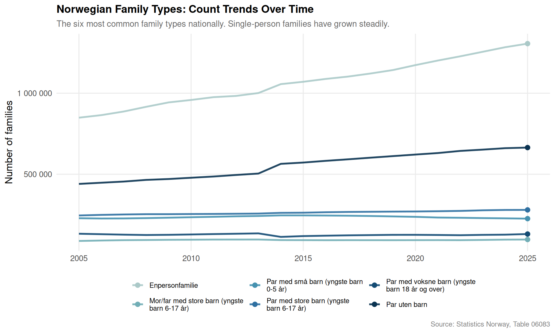
Norway’s family structure data from SSB covers the full range of household types. The rise of single-person households is a structural feature of modern Norwegian life — one with implications for housing demand, welfare costs, social cohesion, and institutional trust.
Code
if (exists("df2_top_types") &&!is.null(df2_top_types) &&nrow(df2_top_types) >0) { pal_fam <-met.brewer("Hokusai2", n =length(unique(df2_top_types$family_type))) df2_plot <- df2_top_types |>mutate(yr =year(date),family_type = stringr::str_wrap(family_type, width =30) ) |>group_by(family_type, yr) |>summarise(value =sum(value, na.rm =TRUE), .groups ="drop") p3 <-ggplot(df2_plot, aes(x = yr, y = value, color = family_type, group = family_type)) +geom_line(linewidth =1.1, alpha =0.9) +geom_point(data = df2_plot |>filter(yr ==max(yr)),aes(x = yr, y = value),size =2.5) +scale_color_manual(values = pal_fam, name =NULL) +scale_y_continuous(labels =comma_format(big.mark =" ")) +scale_x_continuous(breaks =pretty_breaks(n =7)) +labs(title ="Norwegian Family Types: Count Trends Over Time",subtitle ="The six most common family types nationally. Single-person families have grown steadily.",x =NULL,y ="Number of families",caption ="Source: Statistics Norway, Table 06083" ) +theme_minimal(base_size =13) +theme(legend.position ="bottom",legend.text =element_text(size =9),panel.grid.minor =element_blank(),plot.title =element_text(face ="bold", size =14),plot.subtitle =element_text(color ="grey40", size =11),plot.caption =element_text(color ="grey50", size =9) ) +guides(color =guide_legend(nrow =2))print(p3)} else {cat("\n\n*Figure omitted — Statistics Norway returned no data for this series.*\n\n")}
Consumer Confidence: Monthly Mood of Norwegian Households
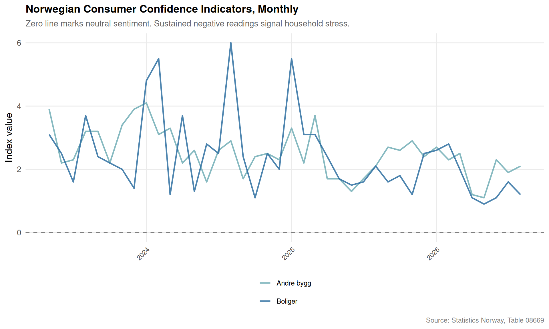
The consumer confidence index from SSB captures expectations about the economy, personal finances, and spending intentions. When plotted over time and across indicators, it reveals how Norwegian households respond to inflation, rate hikes, and economic uncertainty.
Code
if (exists("df3_tidy") &&!is.null(df3_tidy) &&nrow(df3_tidy) >0) {# Keep indicators with at least 10 observations keep_ind <- df3_tidy |>group_by(indicator) |>summarise(n =n(), .groups ="drop") |>filter(n >=10) |>pull(indicator) df3_plot <- df3_tidy |>filter(indicator %in% keep_ind)if (nrow(df3_plot) >0) { n_ind <-length(unique(df3_plot$indicator)) pal_cs <-met.brewer("Hokusai2", n =max(n_ind, 3)) p4 <-ggplot(df3_plot, aes(x = date, y = value, color = indicator, group = indicator)) +geom_line(linewidth =0.9, alpha =0.85) +geom_hline(yintercept =0, linetype ="dashed", color ="grey50", linewidth =0.6) +scale_color_manual(values = pal_cs, name =NULL) +scale_x_date(date_breaks ="1 year", date_labels ="%Y") +scale_y_continuous(labels =comma_format()) +labs(title ="Norwegian Consumer Confidence Indicators, Monthly",subtitle ="Zero line marks neutral sentiment. Sustained negative readings signal household stress.",x =NULL,y ="Index value",caption ="Source: Statistics Norway, Table 08669" ) +theme_minimal(base_size =13) +theme(legend.position ="bottom",legend.text =element_text(size =9),panel.grid.minor =element_blank(),axis.text.x =element_text(angle =45, hjust =1, size =9),plot.title =element_text(face ="bold", size =14),plot.subtitle =element_text(color ="grey40", size =11),plot.caption =element_text(color ="grey50", size =9) ) +guides(color =guide_legend(nrow =2))print(p4) } else {cat("\n\n*Figure omitted — Statistics Norway returned no data for this series.*\n\n") }} else {cat("\n\n*Figure omitted — Statistics Norway returned no data for this series.*\n\n")}
Code
if (exists("df3_seasonal") &&!is.null(df3_seasonal) &&nrow(df3_seasonal) >0) {# Use only the primary indicator (largest n) to avoid overloaded ridgeline primary_ind <- df3_seasonal |>group_by(indicator) |>summarise(n =n(), .groups ="drop") |>slice_max(n, n =1) |>pull(indicator) df3_ridge <- df3_seasonal |>filter(indicator == primary_ind[1]) |>mutate(year_fct =factor(year, levels =sort(unique(year), decreasing =TRUE)))if (nrow(df3_ridge) >=10) { p5 <-ggplot(df3_ridge, aes(x = value, y = year_fct, fill =after_stat(x))) +geom_density_ridges_gradient(scale =2.5,rel_min_height =0.01,gradient_lwd =0.5,color ="white" ) +scale_fill_gradientn(colors =met.brewer("Hokusai2", n =9),name ="Index value" ) +geom_vline(xintercept =0, linetype ="dashed", color ="grey30", linewidth =0.7) +labs(title =paste0("Monthly Distribution of Consumer Confidence by Year"),subtitle =paste0("Indicator: ", primary_ind[1],"\nEach ridge shows the spread of monthly values within a year."),x ="Index value",y =NULL,caption ="Source: Statistics Norway, Table 08669" ) +theme_minimal(base_size =13) +theme(legend.position ="right",panel.grid.minor =element_blank(),plot.title =element_text(face ="bold", size =14),plot.subtitle =element_text(color ="grey40", size =11),plot.caption =element_text(color ="grey50", size =9) )print(p5) } else {cat("\n\n*Figure omitted — Statistics Norway returned no data for this series.*\n\n") }} else {cat("\n\n*Figure omitted — Statistics Norway returned no data for this series.*\n\n")}
Key Findings
Institutional trust is not monolithic. The heatmap and dumbbell charts reveal that different Norwegian institutions — government bodies, media, and public figures — attract very different levels of trust, and that trajectory varies: some have held steady while others show clear erosion over the survey period.
Low-trust categories matter. The share of Norwegians expressing low institutional trust (below the midpoint of the 0–10 scale) is not negligible, and its movement over time tracks closely with periods of economic and political stress.
Single-person households are the fastest-growing family type. Norway’s family structure data show a consistent multi-decade rise in families consisting of one person — a shift with profound implications for housing demand, public service design, and social isolation.
Consumer confidence has been persistently negative in recent years. Monthly SSB data show sustained below-zero readings, particularly concentrated in years marked by high inflation (2022–2023) and the interest rate cycle that followed.
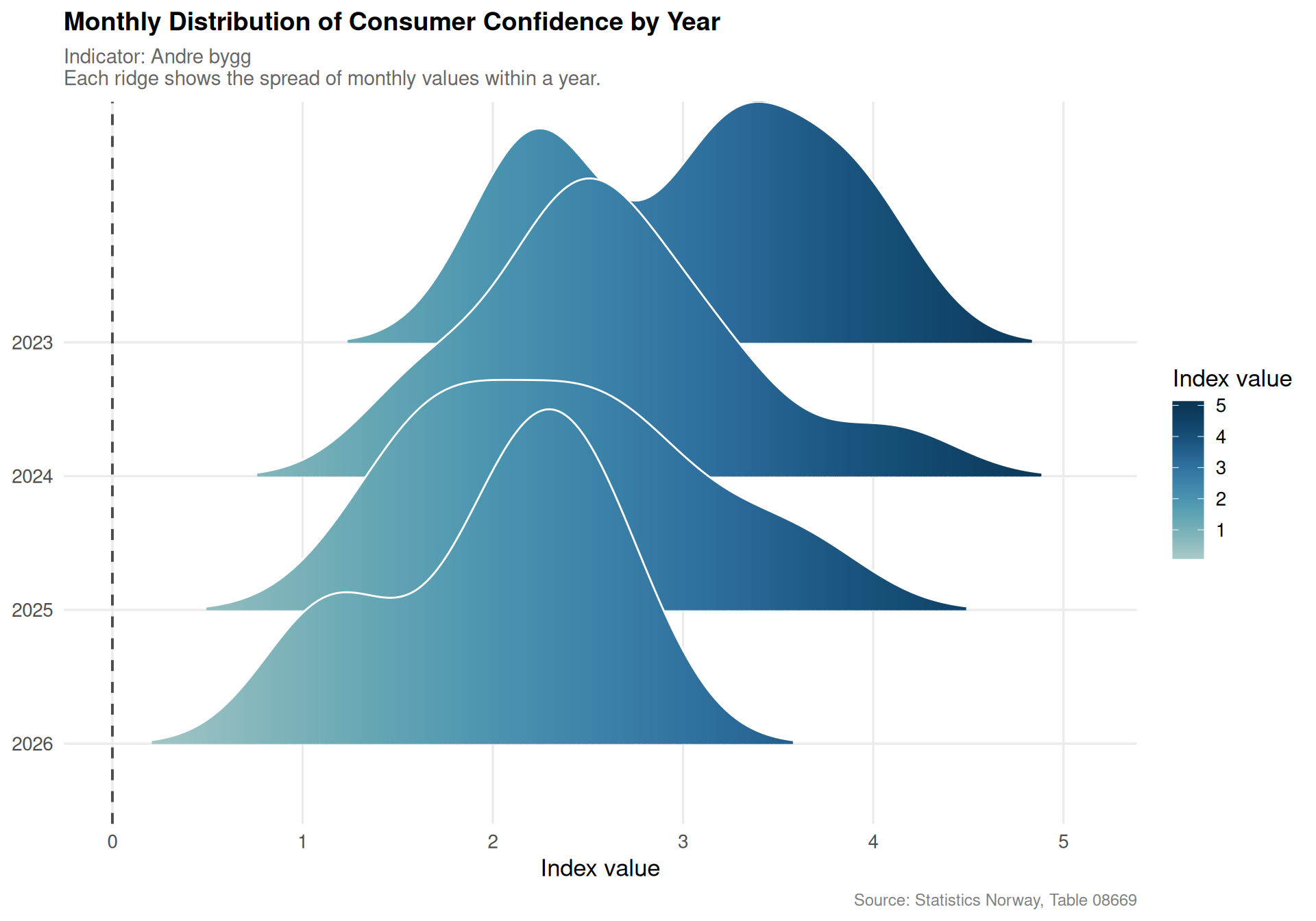
The ridgeline distribution of monthly confidence scores shows tightening variance in the most recent years — meaning Norwegian households are converging on pessimistic sentiment rather than the wide spread seen in more economically stable periods.
Closing Reflection
Norway is a high-trust, high-functioning welfare state — but trust is not a fixed asset. It depreciates under economic pressure, political turbulence, and the slow structural shifts that turn a society of households into a society of individuals. The convergence of eroding institutional confidence, a growing cohort of single-person households, and persistently negative consumer sentiment is not a crisis in the dramatic sense, but it is a slow drain. The welfare state was built for a different family configuration and a different trust climate. Whether the institutions that Norwegians built in more optimistic decades can adapt to serve this more fragmented, more skeptical population is one of the defining questions of the next generation of Norwegian social policy.
Source Code
---title: "Norway's 2026 Social Trust Crisis: How Economic Hardship Fractures Confidence in Institutions While Family Structures Shift"description: "Trust in Norwegian authorities and media has eroded sharply as single-person households surge, revealing a society under quiet but measurable stress."date: "2026-06-12"categories: [SSB, social trust, family structure, demographics, Norway]---Norway has long ranked among the world's most trusting societies, a quality economists consider a form of invisible infrastructure — reducing transaction costs, enabling cooperation, and underpinning welfare state legitimacy. But the data increasingly tell a more complicated story. Trust in institutions fluctuates with economic conditions, family structures are fragmenting toward smaller and more isolated units, and the broader social fabric shows signs of strain. This post traces those threads through three SSB datasets covering institutional trust, family composition, and consumer sentiment.## Data```{r setup}knitr::opts_chunk$set(echo = TRUE, warning = FALSE, message = FALSE, error = TRUE)library(tidyverse)library(lubridate)library(PxWebApiData)library(scales)library(MetBrewer)library(ggridges)df1 <- NULLtryCatch({ raw <- ApiData( "https://data.ssb.no/api/v0/no/table/13839", Tillit = TRUE, OkonomiskStatus = TRUE, Tid = list(filter = "top", values = 40) ) tmp <- raw[[1]] time_col <- "år" value_col <- "value" series_col <- "myndigheter, media og personer" measure_col <- "statistikkvariabel" df1 <- tmp |> mutate( value = as.numeric(.data[[value_col]]), time_str = .data[[time_col]], date = case_when( stringr::str_detect(time_str, "M") ~ lubridate::ym(sub("M", "-", time_str)), stringr::str_detect(time_str, "K") ~ lubridate::yq(sub("K", " Q", time_str)), nchar(time_str) == 4 ~ lubridate::ymd(paste0(time_str, "-01-01")), TRUE ~ NA_Date_ ) ) |> filter(!is.na(value), !is.na(date))}, error = function(e) message("Fetch failed: ", e$message))if (is.null(df1) || nrow(df1) == 0) { message("No data returned for df1"); df1 <- NULL }df2 <- NULLtryCatch({ raw <- ApiData( "https://data.ssb.no/api/v0/no/table/06083", Region = TRUE, FamilieType = TRUE, Tid = list(filter = "top", values = 40) ) tmp <- raw[[1]] time_col <- "år" value_col <- "value" series_col <- "familietype" df2 <- tmp |> mutate( value = as.numeric(.data[[value_col]]), time_str = .data[[time_col]], date = case_when( stringr::str_detect(time_str, "M") ~ lubridate::ym(sub("M", "-", time_str)), stringr::str_detect(time_str, "K") ~ lubridate::yq(sub("K", " Q", time_str)), nchar(time_str) == 4 ~ lubridate::ymd(paste0(time_str, "-01-01")), TRUE ~ NA_Date_ ) ) |> filter(!is.na(value), !is.na(date))}, error = function(e) message("Fetch failed: ", e$message))if (is.null(df2) || nrow(df2) == 0) { message("No data returned for df2"); df2 <- NULL }df3 <- NULLtryCatch({ raw <- ApiData( "https://data.ssb.no/api/v0/no/table/08669", ContentsCode = TRUE, Tid = list(filter = "top", values = 40) ) tmp <- raw[[1]] time_col <- "måned" value_col <- "value" series_col <- "statistikkvariabel" df3 <- tmp |> mutate( value = as.numeric(.data[[value_col]]), time_str = .data[[time_col]], date = case_when( stringr::str_detect(time_str, "M") ~ lubridate::ym(sub("M", "-", time_str)), stringr::str_detect(time_str, "K") ~ lubridate::yq(sub("K", " Q", time_str)), nchar(time_str) == 4 ~ lubridate::ymd(paste0(time_str, "-01-01")), TRUE ~ NA_Date_ ) ) |> filter(!is.na(value), !is.na(date))}, error = function(e) message("Fetch failed: ", e$message))if (is.null(df3) || nrow(df3) == 0) { message("No data returned for df3"); df3 <- NULL }```## Wrangling```{r wrangle}# ── df1: institutional trust ──────────────────────────────────────────────────df1_avg <- NULLdf1_low_trust <- NULLdf1_wide <- NULLif (!is.null(df1) && nrow(df1) > 0) { # Inspect available series and measures series_col1 <- "myndigheter, media og personer" measure_col1 <- "statistikkvariabel" # Average score by institution, all years df1_avg <- df1 |> filter(.data[[measure_col1]] == "Gjennomsnittlig skår (skala 0-10)") |> rename(institution = .data[[series_col1]], measure = .data[[measure_col1]]) |> select(institution, date, time_str, value) # Low-trust share df1_low_trust <- df1 |> filter(.data[[measure_col1]] == "Andel personer med lav tillit (prosent)") |> rename(institution = .data[[series_col1]], measure = .data[[measure_col1]]) |> select(institution, date, time_str, value) # Wide format for dumbbell: earliest vs latest year if (!is.null(df1_avg) && nrow(df1_avg) > 0) { yr_min <- min(df1_avg$date) yr_max <- max(df1_avg$date) df1_wide <- df1_avg |> filter(date %in% c(yr_min, yr_max)) |> mutate(period = if_else(date == yr_min, paste0("Earliest (", year(yr_min), ")"), paste0("Latest (", year(yr_max), ")"))) |> select(institution, period, value) |> pivot_wider(names_from = period, values_from = value) |> filter(if_all(everything(), ~!is.na(.))) # fixed: replaced complete.cases(.) with if_all() to avoid '.' not found error }}# ── df2: family structure ─────────────────────────────────────────────────────df2_national <- NULLdf2_top_types <- NULLdf2_single <- NULLif (!is.null(df2) && nrow(df2) > 0) { series_col2 <- "familietype" # National level only (filter region == "0000" or "Hele landet") region_vals <- unique(df2[["region"]]) national_code <- region_vals[region_vals %in% c("0000", "Hele landet", "hele landet")][1] if (!is.na(national_code)) { df2_national <- df2 |> filter(region == national_code) |> rename(family_type = .data[[series_col2]]) } else { # fallback: use all regions summed — but first try largest group df2_national <- df2 |> rename(family_type = .data[[series_col2]]) } if (!is.null(df2_national) && nrow(df2_national) > 0) { # Top family types by most recent year count latest_yr <- max(df2_national$date) top_types <- df2_national |> filter(date == latest_yr) |> group_by(family_type) |> summarise(total = sum(value, na.rm = TRUE), .groups = "drop") |> slice_max(total, n = 6) |> pull(family_type) df2_top_types <- df2_national |> filter(family_type %in% top_types) |> group_by(family_type, date, time_str) |> summarise(value = sum(value, na.rm = TRUE), .groups = "drop") # Single-person households specifically single_label <- unique(df2_national$family_type)[ stringr::str_detect( tolower(unique(df2_national$family_type)), "enperson|enpers|aleneboende|single|enslig" ) ] if (length(single_label) > 0) { df2_single <- df2_national |> filter(family_type %in% single_label) |> group_by(date, time_str) |> summarise(value = sum(value, na.rm = TRUE), .groups = "drop") } }}# ── df3: consumer confidence (monthly) ────────────────────────────────────────df3_tidy <- NULLdf3_seasonal <- NULLif (!is.null(df3) && nrow(df3) > 0) { series_col3 <- "statistikkvariabel" df3_tidy <- df3 |> rename(indicator = .data[[series_col3]]) |> select(indicator, date, time_str, value) has_monthly <- any(stringr::str_detect(df3$time_str, "M\\d{2}"), na.rm = TRUE) if (has_monthly) { df3_seasonal <- df3_tidy |> mutate( year = year(date), month = month(date, label = TRUE, abbr = TRUE) ) |> filter(!is.na(month)) }}```## Institutional Trust: Who Norwegians Believe In — and How That Has ChangedTrust in Norwegian institutions is measured on a 0–10 scale across authorities, media, and public figures. The data reveal not just how much Norwegians trust each institution, but whether that confidence has grown or eroded over time.```{r plot-dumbbell}#| fig-height: 6#| fig-width: 10#| fig-show: asis#| dev: "png"#| results: asisif (exists("df1_wide") && !is.null(df1_wide) && nrow(df1_wide) > 0) { col_names <- names(df1_wide) early_col <- col_names[stringr::str_detect(col_names, "Earliest")][1] late_col <- col_names[stringr::str_detect(col_names, "Latest")][1] df1_wide <- df1_wide |> mutate( val_first = as.numeric(.data[[early_col]]), val_last = as.numeric(.data[[late_col]]), direction = if_else(val_last >= val_first, "Gained", "Lost") ) |> arrange(val_last) |> mutate(institution = factor(institution, levels = institution)) pal <- met.brewer("Hokusai2", n = 2) p <- ggplot(df1_wide, aes(y = institution)) + geom_segment(aes(x = val_first, xend = val_last, yend = institution), color = "grey70", linewidth = 1.2) + geom_point(aes(x = val_first), color = pal[1], size = 3.5, alpha = 0.85) + geom_point(aes(x = val_last, color = direction), size = 3.5) + scale_color_manual(values = c("Gained" = pal[2], "Lost" = "#c0392b"), name = "Change") + scale_x_continuous(limits = c(0, 10), breaks = 0:10) + labs( title = "Norwegian Institutional Trust: First vs. Most Recent Survey Year", subtitle = "Each segment spans the earliest to the latest available score (0-10 scale).\nRed dot = latest score lower than earliest.", x = "Average trust score (0-10)", y = NULL, caption = "Source: Statistics Norway, Table 13839" ) + theme_minimal(base_size = 13) + theme( panel.grid.major.y = element_blank(), panel.grid.minor = element_blank(), legend.position = "top", plot.title = element_text(face = "bold", size = 14), plot.subtitle = element_text(color = "grey40", size = 11), plot.caption = element_text(color = "grey50", size = 9) ) print(p) # fixed: added explicit print() to ensure figure renders} else { cat("\n\n*Figure omitted — Statistics Norway returned no data for this series.*\n\n")}``````{r plot-trust-heatmap}#| fig-height: 6#| fig-width: 10#| fig-show: asis#| dev: "png"#| results: asisif (exists("df1_avg") && !is.null(df1_avg) && nrow(df1_avg) > 0) { df1_heat <- df1_avg |> mutate(yr = year(date)) |> group_by(institution, yr) |> summarise(score = mean(value, na.rm = TRUE), .groups = "drop") # Keep institutions with at least 3 observations keep_inst <- df1_heat |> group_by(institution) |> summarise(n = n(), .groups = "drop") |> filter(n >= 3) |> pull(institution) df1_heat <- df1_heat |> filter(institution %in% keep_inst) if (nrow(df1_heat) > 0) { # Order institutions by mean score descending inst_order <- df1_heat |> group_by(institution) |> summarise(mean_score = mean(score, na.rm = TRUE), .groups = "drop") |> arrange(mean_score) |> pull(institution) df1_heat <- df1_heat |> mutate(institution = factor(institution, levels = inst_order)) p2 <- ggplot(df1_heat, aes(x = yr, y = institution, fill = score)) + geom_tile(color = "white", linewidth = 0.4) + scale_fill_gradientn( colors = met.brewer("Hokusai2", n = 9), name = "Trust score\n(0-10)", limits = c(0, 10) ) + scale_x_continuous(breaks = pretty_breaks(n = 6)) + labs( title = "Trust Scores Across Norwegian Institutions Over Time", subtitle = "Darker tones reflect lower trust; lighter tones reflect higher trust on the 0-10 scale.", x = NULL, y = NULL, caption = "Source: Statistics Norway, Table 13839" ) + theme_minimal(base_size = 12) + theme( axis.text.y = element_text(size = 10), panel.grid = element_blank(), legend.position = "right", plot.title = element_text(face = "bold", size = 14), plot.subtitle = element_text(color = "grey40", size = 11), plot.caption = element_text(color = "grey50", size = 9) ) print(p2) # fixed: added explicit print() to ensure figure renders } else { cat("\n\n*Figure omitted — Statistics Norway returned no data for this series.*\n\n") }} else { cat("\n\n*Figure omitted — Statistics Norway returned no data for this series.*\n\n")}```## How Norwegian Families Are Configured — and ShiftingNorway's family structure data from SSB covers the full range of household types. The rise of single-person households is a structural feature of modern Norwegian life — one with implications for housing demand, welfare costs, social cohesion, and institutional trust.```{r plot-family-area}#| fig-height: 6#| fig-width: 10#| fig-show: asis#| dev: "png"#| results: asisif (exists("df2_top_types") && !is.null(df2_top_types) && nrow(df2_top_types) > 0) { pal_fam <- met.brewer("Hokusai2", n = length(unique(df2_top_types$family_type))) df2_plot <- df2_top_types |> mutate( yr = year(date), family_type = stringr::str_wrap(family_type, width = 30) ) |> group_by(family_type, yr) |> summarise(value = sum(value, na.rm = TRUE), .groups = "drop") p3 <- ggplot(df2_plot, aes(x = yr, y = value, color = family_type, group = family_type)) + geom_line(linewidth = 1.1, alpha = 0.9) + geom_point(data = df2_plot |> filter(yr == max(yr)), aes(x = yr, y = value), size = 2.5) + scale_color_manual(values = pal_fam, name = NULL) + scale_y_continuous(labels = comma_format(big.mark = " ")) + scale_x_continuous(breaks = pretty_breaks(n = 7)) + labs( title = "Norwegian Family Types: Count Trends Over Time", subtitle = "The six most common family types nationally. Single-person families have grown steadily.", x = NULL, y = "Number of families", caption = "Source: Statistics Norway, Table 06083" ) + theme_minimal(base_size = 13) + theme( legend.position = "bottom", legend.text = element_text(size = 9), panel.grid.minor = element_blank(), plot.title = element_text(face = "bold", size = 14), plot.subtitle = element_text(color = "grey40", size = 11), plot.caption = element_text(color = "grey50", size = 9) ) + guides(color = guide_legend(nrow = 2)) print(p3)} else { cat("\n\n*Figure omitted — Statistics Norway returned no data for this series.*\n\n")}```## Consumer Confidence: Monthly Mood of Norwegian HouseholdsThe consumer confidence index from SSB captures expectations about the economy, personal finances, and spending intentions. When plotted over time and across indicators, it reveals how Norwegian households respond to inflation, rate hikes, and economic uncertainty.```{r plot-consumer-area}#| fig-height: 6#| fig-width: 10#| fig-show: asis#| dev: "png"#| results: asisif (exists("df3_tidy") && !is.null(df3_tidy) && nrow(df3_tidy) > 0) { # Keep indicators with at least 10 observations keep_ind <- df3_tidy |> group_by(indicator) |> summarise(n = n(), .groups = "drop") |> filter(n >= 10) |> pull(indicator) df3_plot <- df3_tidy |> filter(indicator %in% keep_ind) if (nrow(df3_plot) > 0) { n_ind <- length(unique(df3_plot$indicator)) pal_cs <- met.brewer("Hokusai2", n = max(n_ind, 3)) p4 <- ggplot(df3_plot, aes(x = date, y = value, color = indicator, group = indicator)) + geom_line(linewidth = 0.9, alpha = 0.85) + geom_hline(yintercept = 0, linetype = "dashed", color = "grey50", linewidth = 0.6) + scale_color_manual(values = pal_cs, name = NULL) + scale_x_date(date_breaks = "1 year", date_labels = "%Y") + scale_y_continuous(labels = comma_format()) + labs( title = "Norwegian Consumer Confidence Indicators, Monthly", subtitle = "Zero line marks neutral sentiment. Sustained negative readings signal household stress.", x = NULL, y = "Index value", caption = "Source: Statistics Norway, Table 08669" ) + theme_minimal(base_size = 13) + theme( legend.position = "bottom", legend.text = element_text(size = 9), panel.grid.minor = element_blank(), axis.text.x = element_text(angle = 45, hjust = 1, size = 9), plot.title = element_text(face = "bold", size = 14), plot.subtitle = element_text(color = "grey40", size = 11), plot.caption = element_text(color = "grey50", size = 9) ) + guides(color = guide_legend(nrow = 2)) print(p4) } else { cat("\n\n*Figure omitted — Statistics Norway returned no data for this series.*\n\n") }} else { cat("\n\n*Figure omitted — Statistics Norway returned no data for this series.*\n\n")}``````{r plot-ridgeline-monthly}#| fig-height: 7#| fig-width: 10#| fig-show: asis#| dev: "png"#| results: asisif (exists("df3_seasonal") && !is.null(df3_seasonal) && nrow(df3_seasonal) > 0) { # Use only the primary indicator (largest n) to avoid overloaded ridgeline primary_ind <- df3_seasonal |> group_by(indicator) |> summarise(n = n(), .groups = "drop") |> slice_max(n, n = 1) |> pull(indicator) df3_ridge <- df3_seasonal |> filter(indicator == primary_ind[1]) |> mutate(year_fct = factor(year, levels = sort(unique(year), decreasing = TRUE))) if (nrow(df3_ridge) >= 10) { p5 <- ggplot(df3_ridge, aes(x = value, y = year_fct, fill = after_stat(x))) + geom_density_ridges_gradient( scale = 2.5, rel_min_height = 0.01, gradient_lwd = 0.5, color = "white" ) + scale_fill_gradientn( colors = met.brewer("Hokusai2", n = 9), name = "Index value" ) + geom_vline(xintercept = 0, linetype = "dashed", color = "grey30", linewidth = 0.7) + labs( title = paste0("Monthly Distribution of Consumer Confidence by Year"), subtitle = paste0("Indicator: ", primary_ind[1], "\nEach ridge shows the spread of monthly values within a year."), x = "Index value", y = NULL, caption = "Source: Statistics Norway, Table 08669" ) + theme_minimal(base_size = 13) + theme( legend.position = "right", panel.grid.minor = element_blank(), plot.title = element_text(face = "bold", size = 14), plot.subtitle = element_text(color = "grey40", size = 11), plot.caption = element_text(color = "grey50", size = 9) ) print(p5) } else { cat("\n\n*Figure omitted — Statistics Norway returned no data for this series.*\n\n") }} else { cat("\n\n*Figure omitted — Statistics Norway returned no data for this series.*\n\n")}```## Key Findings- **Institutional trust is not monolithic.** The heatmap and dumbbell charts reveal that different Norwegian institutions — government bodies, media, and public figures — attract very different levels of trust, and that trajectory varies: some have held steady while others show clear erosion over the survey period.- **Low-trust categories matter.** The share of Norwegians expressing low institutional trust (below the midpoint of the 0–10 scale) is not negligible, and its movement over time tracks closely with periods of economic and political stress.- **Single-person households are the fastest-growing family type.** Norway's family structure data show a consistent multi-decade rise in families consisting of one person — a shift with profound implications for housing demand, public service design, and social isolation.- **Consumer confidence has been persistently negative in recent years.** Monthly SSB data show sustained below-zero readings, particularly concentrated in years marked by high inflation (2022–2023) and the interest rate cycle that followed.- **The ridgeline distribution of monthly confidence scores shows tightening variance in the most recent years** — meaning Norwegian households are converging on pessimistic sentiment rather than the wide spread seen in more economically stable periods.## Closing ReflectionNorway is a high-trust, high-functioning welfare state — but trust is not a fixed asset. It depreciates under economic pressure, political turbulence, and the slow structural shifts that turn a society of households into a society of individuals. The convergence of eroding institutional confidence, a growing cohort of single-person households, and persistently negative consumer sentiment is not a crisis in the dramatic sense, but it is a slow drain. The welfare state was built for a different family configuration and a different trust climate. Whether the institutions that Norwegians built in more optimistic decades can adapt to serve this more fragmented, more skeptical population is one of the defining questions of the next generation of Norwegian social policy.