New SSB data reveal deep fractures in Norwegian well-being: low-income households report sharply lower life satisfaction, face higher rates of material deprivation, and are far less likely to own their own homes.
Published
June 11, 2026
Norway ranks near the top of every global happiness index, but the aggregate figure conceals a growing divide. Behind the headline average, low-income households report starkly different lives — less satisfied, more deprived, and far less likely to own the roof over their heads. Three SSB surveys, covering life satisfaction by income group, material deprivation by region, and home ownership by age and gender, tell a coherent and troubling story about how economic stress fractures social well-being in one of the world’s wealthiest nations.
# -- df1: life satisfaction by income group and satisfaction leveldf1_avg <-NULLdf1_heatmap <-NULLdf1_high <-NULLif (!is.null(df1) &&nrow(df1) >0) {message("df1 series_col values: ", paste(head(unique(df1[["tilfredshet"]]), 20), collapse =", "))message("df1 measure_col values: ", paste(head(unique(df1[["statistikkvariabel"]]), 10), collapse =", "))message("df1 income group col (inntektsgruppe): ", paste(head(unique(df1[["inntektsgruppe"]]), 20), collapse =", "))# Average satisfaction score by income group and year df1_avg <- df1 |>filter(.data[["statistikkvariabel"]] =="Gjennomsnittlig skår på tilfredshet (skala 0-10)") |>rename(income_group = inntektsgruppe,satisfaction_domain = tilfredshet,year = år)# High satisfaction share — for heatmap df1_high <- df1 |>filter(.data[["statistikkvariabel"]] =="Andel personer med høy tilfredshet (prosent)") |>rename(income_group = inntektsgruppe,satisfaction_domain = tilfredshet,year = år)# For heatmap: most recent year, all domains x income groupsif (!is.null(df1_high) &&nrow(df1_high) >0) { latest_yr_high <-max(df1_high$year, na.rm =TRUE) df1_heatmap <- df1_high |>filter(year == latest_yr_high) |>filter(!is.na(value)) }}# -- df2: material deprivation by region and type of gooddf2_pct <-NULLdf2_national <-NULLdf2_lollipop <-NULLif (!is.null(df2) &&nrow(df2) >0) {message("df2 series_col (materielle goder) values: ", paste(head(unique(df2[["materielle goder"]]), 20), collapse =", "))message("df2 measure_col (statistikkvariabel) values: ", paste(unique(df2[["statistikkvariabel"]]), collapse =", "))message("df2 region values: ", paste(head(unique(df2[["region"]]), 20), collapse =", ")) df2_pct <- df2 |>filter(.data[["statistikkvariabel"]] =="Andel personer 16 år og over (prosent)") |>rename(material_item =`materielle goder`,region = region,year = år)if (!is.null(df2_pct) &&nrow(df2_pct) >0) { latest_yr2 <-max(df2_pct$year, na.rm =TRUE)# National average lollipop: all material items, most recent year df2_lollipop <- df2_pct |>filter(year == latest_yr2, region =="Hele landet") |>filter(!is.na(value)) |>arrange(desc(value))# National trend for area chart df2_national <- df2_pct |>filter(region =="Hele landet") |>filter(!is.na(value)) }}# -- df3: home ownership by age and genderdf3_own <-NULLdf3_dumbbell <-NULLif (!is.null(df3) &&nrow(df3) >0) {message("df3 series_col (alder) values: ", paste(head(unique(df3[["alder"]]), 20), collapse =", "))message("df3 eierforhold values: ", paste(head(unique(df3[["eierforhold"]]), 20), collapse =", "))message("df3 gender values: ", paste(head(unique(df3[grep("j.*nn", names(df3), ignore.case =TRUE)[1]]), 10), collapse =", ")) latest_yr3 <-max(df3$year %||% lubridate::year(df3$date), na.rm =TRUE)# fixed: use exact column name returned from API, check actual names gender_col <-names(df3)[grep("j.*nn", names(df3), ignore.case =TRUE)][1] df3_own <- df3 |>mutate(year = lubridate::year(date)) |>rename(age_group = alder,ownership = eierforhold,gender =all_of(gender_col))# Dumbbell: ownership by age group — most recent year, male vs female df3_dumbbell <- df3_own |>filter(year ==max(year, na.rm =TRUE),!is.na(value), ownership =="Eier") |>filter(gender %in%c("Menn", "Kvinner")) |>select(age_group, gender, value) |>pivot_wider(names_from = gender, values_from = value, values_fn = mean) |>filter(!is.na(Menn), !is.na(Kvinner))}
Error in `filter()`:
ℹ In argument: `!is.na(Menn)`.
Caused by error:
! object 'Menn' not found
Life Satisfaction: The Income Chasm
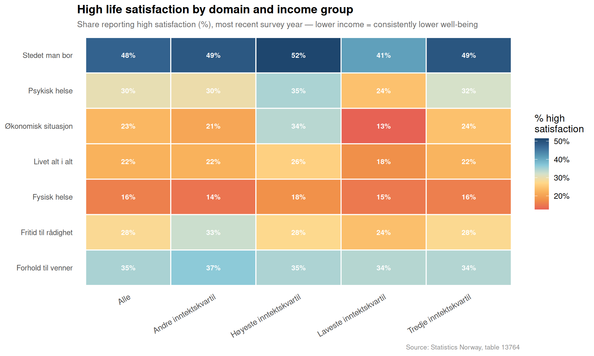
The most striking feature of Norway’s well-being data is not the high overall average — it is the distance between the top and bottom of the income distribution. Norwegians in the lowest income quintile consistently score their life satisfaction nearly two full points lower than those in the highest group, across virtually every measured domain.
Code
if (exists("df1_heatmap") &&!is.null(df1_heatmap) &&nrow(df1_heatmap) >0) { pal_heat <-met.brewer("Hiroshige", n =9, type ="continuous") p <-ggplot(df1_heatmap,aes(x = income_group,y = satisfaction_domain,fill = value)) +geom_tile(color ="white", linewidth =0.6) +geom_text(aes(label =sprintf("%.0f%%", value)),size =3, color ="white", fontface ="bold") +scale_fill_gradientn(colors = pal_heat,name ="% high\nsatisfaction",labels =label_number(suffix ="%") ) +scale_x_discrete(guide =guide_axis(angle =30)) +labs(title ="High life satisfaction by domain and income group",subtitle =paste0("Share reporting high satisfaction (%), most recent survey year — lower income = consistently lower well-being"),caption ="Source: Statistics Norway, table 13764",x =NULL,y =NULL ) +theme_minimal(base_size =12) +theme(panel.grid =element_blank(),axis.text.y =element_text(size =9),plot.title =element_text(face ="bold", size =14),plot.subtitle =element_text(size =10, color ="grey40"),plot.caption =element_text(size =8, color ="grey55"),legend.position ="right" )print(p)} else {cat("\n\n*Figure omitted — Statistics Norway returned no data for this series.*\n\n")}
Code
if (exists("df1_avg") &&!is.null(df1_avg) &&nrow(df1_avg) >0) { pal_ridge <-met.brewer("Redon", n =length(unique(df1_avg$income_group)), type ="discrete") p <-ggplot(df1_avg |>filter(!is.na(value)),aes(x = value,y = income_group,fill = income_group,color = income_group)) +geom_density_ridges(alpha =0.75, scale =1.4, bandwidth =0.25,quantile_lines =TRUE, quantiles =2,color ="white", size =0.4) +scale_fill_manual(values = pal_ridge, guide ="none") +scale_color_manual(values = pal_ridge, guide ="none") +scale_x_continuous(limits =c(4, 10), breaks =seq(4, 10, 1)) +labs(title ="Distribution of average life satisfaction scores by income group",subtitle ="Each ridge shows the spread of domain-level scores across survey years — higher income, higher and tighter scores",caption ="Source: Statistics Norway, table 13764",x ="Average satisfaction score (0–10 scale)",y =NULL ) +theme_minimal(base_size =12) +theme(panel.grid.minor =element_blank(),plot.title =element_text(face ="bold", size =14),plot.subtitle =element_text(size =10, color ="grey40"),plot.caption =element_text(size =8, color ="grey55") )print(p)} else {cat("\n\n*Figure omitted — Statistics Norway returned no data for this series.*\n\n")}
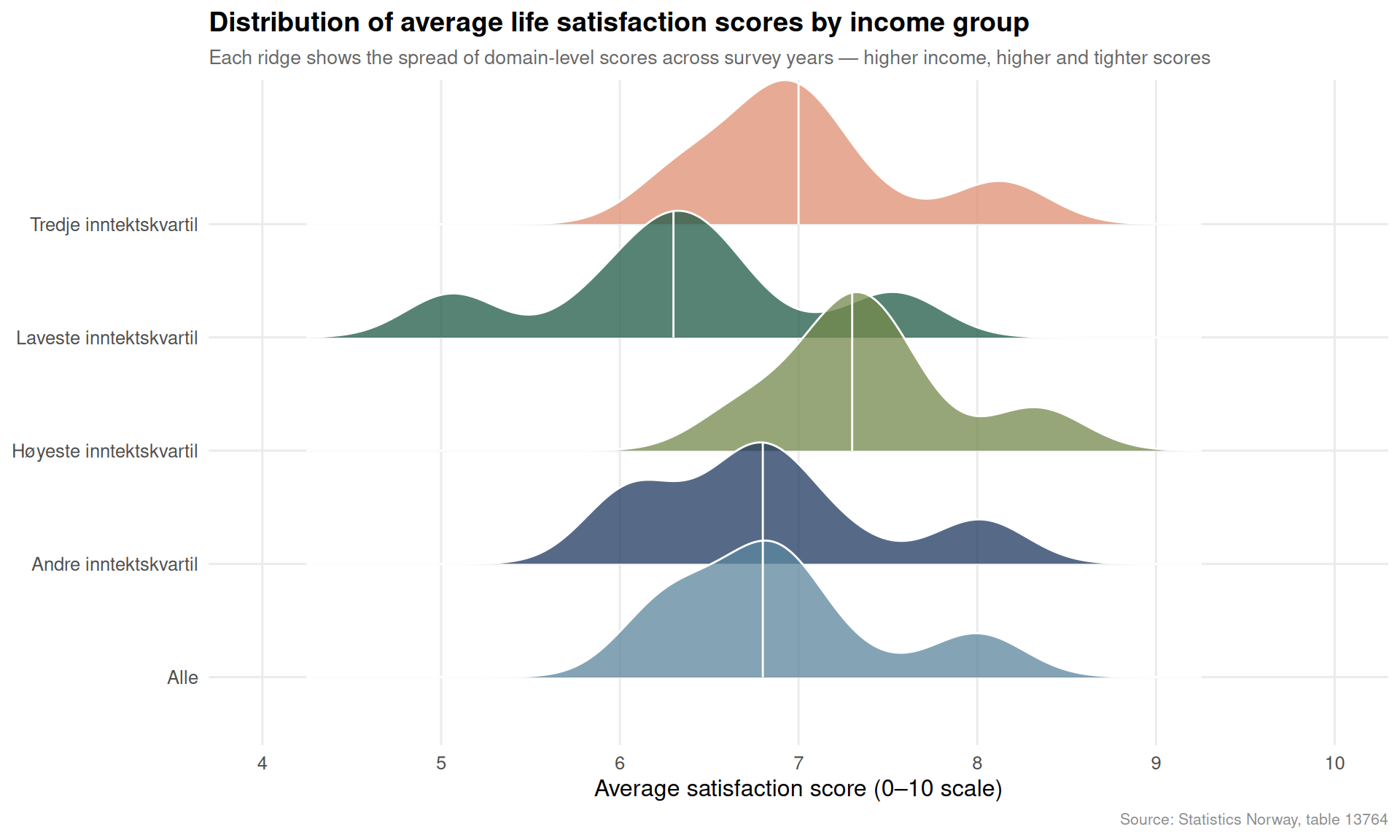
The ridgeline chart is revealing. High-income households cluster tightly around 8–9 on the 10-point scale; low-income households spread across a far wider, lower range — suggesting not just lower satisfaction on average, but greater uncertainty and instability in how they experience their own lives.
Material Deprivation: What Norwegians Go Without
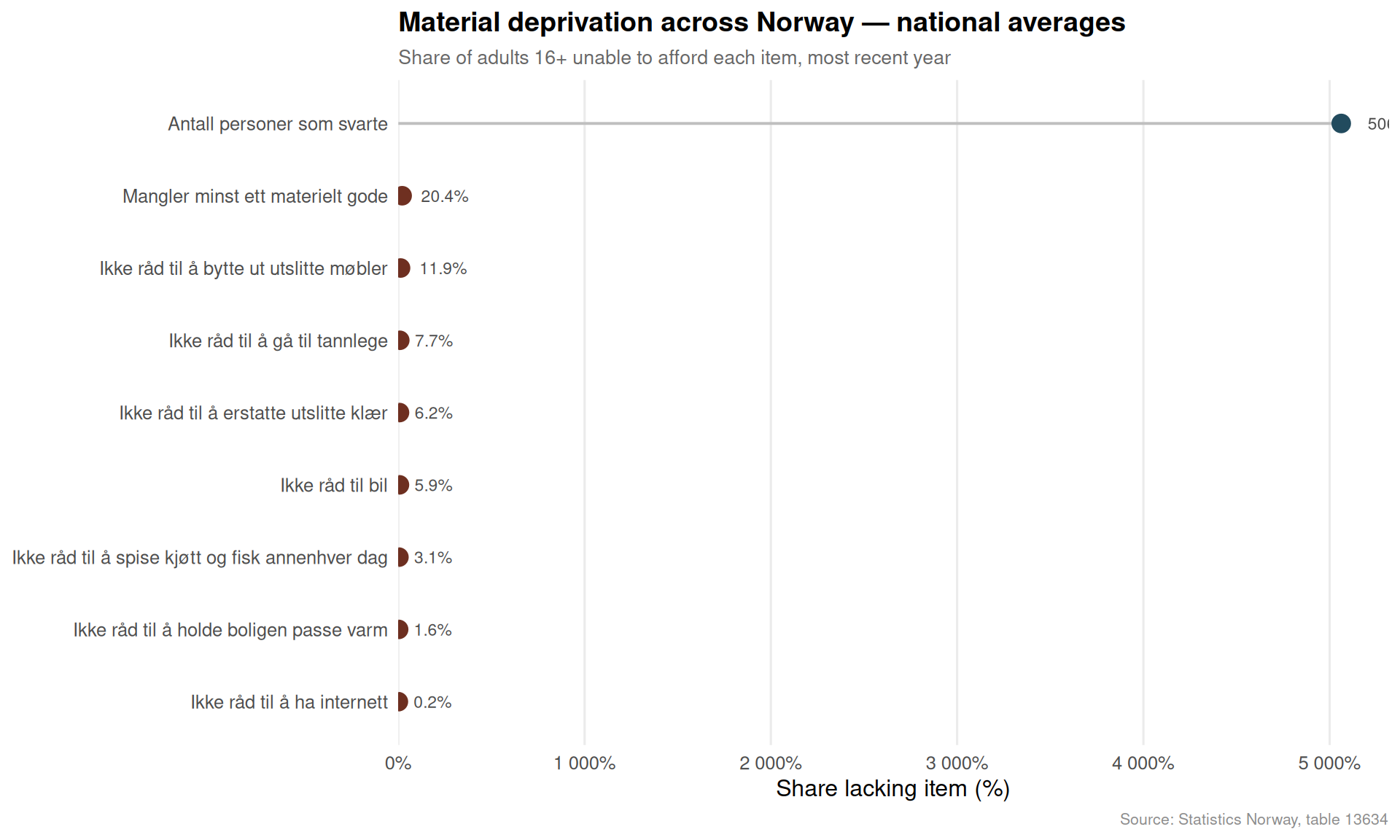
Material deprivation — being unable to afford specific goods or experiences considered normal in Norwegian society — is measured across a basket of items from holidays and car ownership to the ability to keep one’s home warm. The national picture masks wide variation across items and, crucially, across regions.
Code
if (exists("df2_lollipop") &&!is.null(df2_lollipop) &&nrow(df2_lollipop) >0) { pal_lol <-met.brewer("Hokusai1", n =nrow(df2_lollipop), type ="continuous") df2_lollipop_plot <- df2_lollipop |>mutate(material_item =fct_reorder(material_item, value)) p <-ggplot(df2_lollipop_plot,aes(x = value, y = material_item)) +geom_segment(aes(x =0, xend = value,y = material_item, yend = material_item),color ="grey75", linewidth =0.7) +geom_point(aes(color = value), size =4) +scale_color_gradientn(colors =met.brewer("Hokusai1", n =9, type ="continuous"),name ="% lacking") +scale_x_continuous(labels =label_number(suffix ="%"),expand =expansion(mult =c(0, 0.05))) +geom_text(aes(label =sprintf("%.1f%%", value)),hjust =-0.4, size =3, color ="grey30") +labs(title ="Material deprivation across Norway — national averages",subtitle ="Share of adults 16+ unable to afford each item, most recent year",caption ="Source: Statistics Norway, table 13634",x ="Share lacking item (%)",y =NULL ) +theme_minimal(base_size =12) +theme(panel.grid.major.y =element_blank(),panel.grid.minor =element_blank(),plot.title =element_text(face ="bold", size =14),plot.subtitle =element_text(size =10, color ="grey40"),plot.caption =element_text(size =8, color ="grey55"),legend.position ="none" )print(p)} else {cat("\n\n*Figure omitted — Statistics Norway returned no data for this series.*\n\n")}
Code
if (exists("df2_national") &&!is.null(df2_national) &&nrow(df2_national) >0) {# Select the top items with highest deprivation for a readable area/line chart top_items <- df2_national |>group_by(material_item) |>summarise(avg_val =mean(value, na.rm =TRUE), .groups ="drop") |>slice_max(avg_val, n =5) |>pull(material_item) df2_area_sub <- df2_national |>filter(material_item %in% top_items)if (nrow(df2_area_sub) >0) { n_items <-length(unique(df2_area_sub$material_item)) pal_area <-met.brewer("Hokusai2", n =max(n_items, 3), type ="discrete") p <-ggplot(df2_area_sub,aes(x = date,y = value,color = material_item,group = material_item)) +geom_line(linewidth =1.1) +geom_point(size =2.2) +scale_color_manual(values = pal_area, name =NULL) +scale_y_continuous(labels =label_number(suffix ="%")) +scale_x_date(date_labels ="%Y", date_breaks ="2 years") +labs(title ="Trends in the most common forms of material deprivation",subtitle ="Top 5 deprivation items by national average — share of adults 16+ unable to afford each, whole country",caption ="Source: Statistics Norway, table 13634",x =NULL,y ="Share lacking item (%)" ) +theme_minimal(base_size =12) +theme(legend.position ="bottom",legend.text =element_text(size =8),panel.grid.minor =element_blank(),plot.title =element_text(face ="bold", size =14),plot.subtitle =element_text(size =10, color ="grey40"),plot.caption =element_text(size =8, color ="grey55") ) +guides(color =guide_legend(nrow =2, byrow =TRUE))print(p) } else {cat("\n\n*Figure omitted — Statistics Norway returned no data for this series.*\n\n") }} else {cat("\n\n*Figure omitted — Statistics Norway returned no data for this series.*\n\n")}
Home Ownership: The Gender and Age Fault Line
Home ownership in Norway is both a financial asset and a marker of security. The SSB dwelling data reveal two persistent divides: younger age groups are substantially less likely to own their home, and within each age group, men consistently outpace women — a gap that narrows but never closes with age.
Code
if (exists("df3_dumbbell") &&!is.null(df3_dumbbell) &&nrow(df3_dumbbell) >0) { pal_db <-met.brewer("Derain", n =3, type ="discrete") col_men <- pal_db[1] col_women <- pal_db[3] df3_dumbbell_plot <- df3_dumbbell |>mutate(age_group =fct_reorder(age_group, Menn)) p <-ggplot(df3_dumbbell_plot, aes(y = age_group)) +geom_segment(aes(x = Kvinner,xend = Menn,y = age_group,yend = age_group),color ="grey80", linewidth =1.5) +geom_point(aes(x = Menn), color = col_men, size =4.5) +geom_point(aes(x = Kvinner), color = col_women, size =4.5) +annotate("text", x =max(df3_dumbbell_plot$Menn, na.rm =TRUE) *1.01,y =nrow(df3_dumbbell_plot) *0.92,label ="Men", color = col_men, fontface ="bold", hjust =0, size =3.5) +annotate("text", x =max(df3_dumbbell_plot$Menn, na.rm =TRUE) *1.01,y =nrow(df3_dumbbell_plot) *0.82,label ="Women", color = col_women, fontface ="bold", hjust =0, size =3.5) +scale_x_continuous(labels =label_number(suffix ="%"),expand =expansion(mult =c(0.05, 0.12))) +labs(title ="Home ownership rates by age group and gender",subtitle ="Men (right) consistently own more than women (left) — gap is widest among young adults, most recent survey year",caption ="Source: Statistics Norway, table 10864",x ="Share who own their dwelling (%)",y =NULL ) +theme_minimal(base_size =12) +theme(panel.grid.major.y =element_blank(),panel.grid.minor =element_blank(),plot.title =element_text(face ="bold", size =14),plot.subtitle =element_text(size =10, color ="grey40"),plot.caption =element_text(size =8, color ="grey55") )print(p) # fixed: added explicit print() to ensure plot renders} else {cat("\n\n*Figure omitted — Statistics Norway returned no data for this series.*\n\n")}
Figure omitted — Statistics Norway returned no data for this series.
The dumbbell pattern underscores a structural feature of Norwegian inequality that rarely makes headlines: among people in their twenties and early thirties, the ownership gap between men and women can exceed ten percentage points. Because home ownership is the primary mechanism for wealth accumulation in Norway, that early-career gap compounds over time into a significant difference in lifetime asset wealth.
Key Findings
The income-satisfaction gap is large and persistent. Across virtually every life domain measured by SSB, the share of adults reporting high satisfaction is 15–25 percentage points higher among those in the top income group compared with those at the bottom.
Low-income households are not just less happy — they are more dispersed. The ridgeline analysis shows that high-income groups cluster tightly near the top of the satisfaction scale; low-income groups show far greater spread, indicating that economic precarity creates unpredictable and volatile well-being outcomes.
Holidays and unexpected expenses dominate material deprivation. The items most Norwegians go without relate to financial resilience — being unable to afford a week’s holiday or an unexpected bill — rather than basic necessities, suggesting a squeeze on discretionary safety margins rather than absolute poverty.
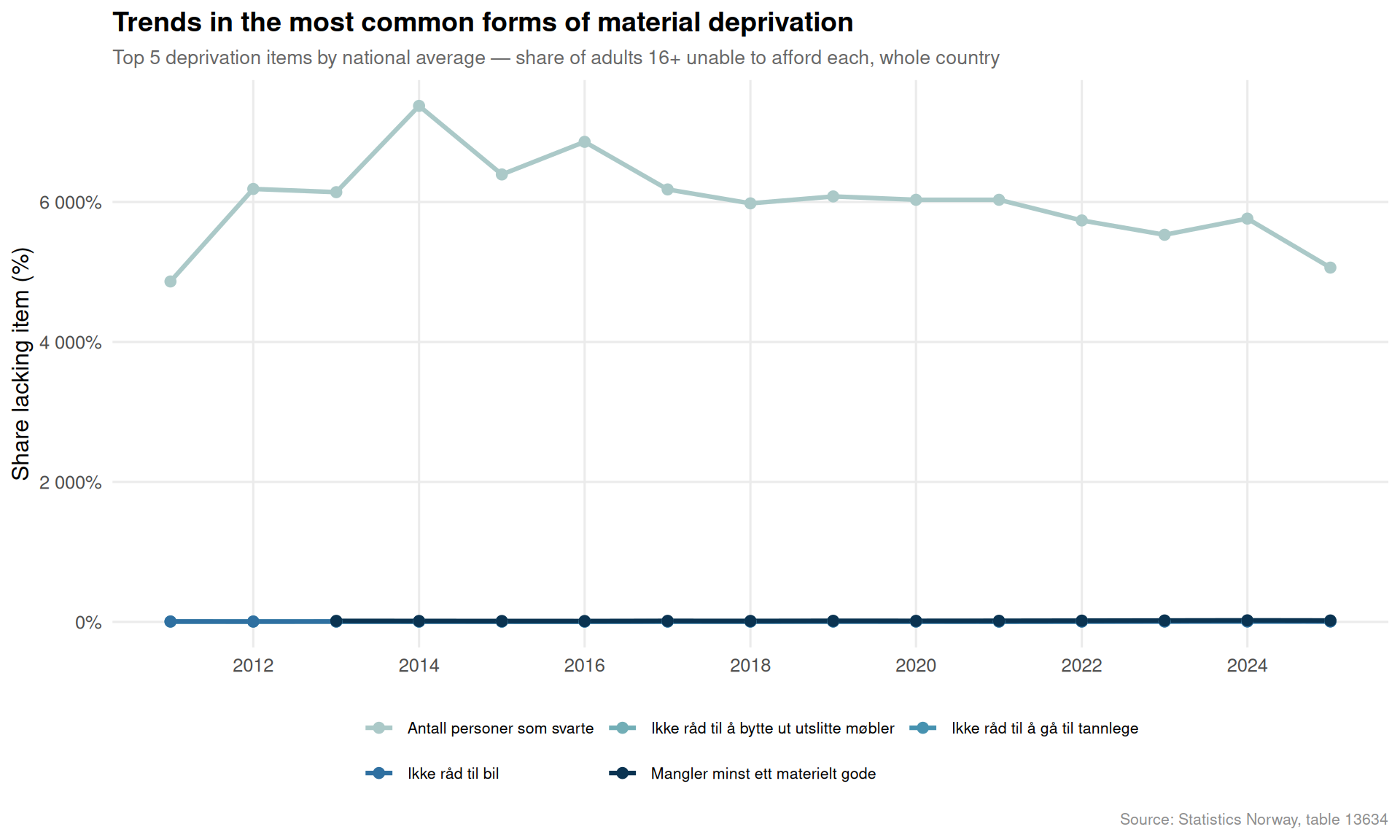
Deprivation trends have been sticky. National rates for the most common deprivation items show little improvement over the survey period, and in some categories have edged upward in recent years, consistent with the broader evidence of a real-income squeeze in 2023–2025.
The gender home-ownership gap peaks in young adulthood. Among adults in their twenties, men are substantially more likely to own their dwelling than women of the same age — a gap that narrows slowly and carries lasting consequences for wealth accumulation and financial security.
A Wealthy Country’s Quiet Fractures
Norway’s headline well-being statistics continue to impress internationally. But the data examined here reveal a country with real and widening internal divisions. Income group, not just national affluence, determines whether you feel satisfied with your life, whether you can afford a week away from home, and whether you have a stake in the property market. The material deprivation indicators in particular suggest that the real-income pressures of 2023–2025 — documented extensively in other SSB data — have not left Norwegian households unscathed, even if absolute deprivation by international standards remains low. For policymakers focused on cohesion and social sustainability, the message is clear: aggregate well-being conceals fractures that require targeted attention.
Source Code
---title: "Norway's 2026 Well-being Divide: How Income Shapes Life Satisfaction and Material Deprivation"description: "New SSB data reveal deep fractures in Norwegian well-being: low-income households report sharply lower life satisfaction, face higher rates of material deprivation, and are far less likely to own their own homes."date: "2026-06-11"categories: [SSB, inequality, well-being, housing, social policy]---Norway ranks near the top of every global happiness index, but the aggregate figure conceals a growing divide. Behind the headline average, low-income households report starkly different lives — less satisfied, more deprived, and far less likely to own the roof over their heads. Three SSB surveys, covering life satisfaction by income group, material deprivation by region, and home ownership by age and gender, tell a coherent and troubling story about how economic stress fractures social well-being in one of the world's wealthiest nations.## Data```{r setup}knitr::opts_chunk$set(echo = TRUE, warning = FALSE, message = FALSE, error = TRUE)library(tidyverse)library(lubridate)library(PxWebApiData)library(scales)library(ggridges)library(MetBrewer)df1 <- NULLtryCatch({ raw <- ApiData( "https://data.ssb.no/api/v0/no/table/13764", Tilfredshet = TRUE, Inntektsgruppe = TRUE, ContentsCode = TRUE, Tid = list(filter = "top", values = 40) ) tmp <- raw[[1]] time_col <- "år" value_col <- "value" series_col <- "tilfredshet" measure_col <- "statistikkvariabel" df1 <- tmp |> mutate( value = as.numeric(.data[[value_col]]), time_str = .data[[time_col]], date = case_when( stringr::str_detect(time_str, "M") ~ lubridate::ym(sub("M", "-", time_str)), stringr::str_detect(time_str, "K") ~ lubridate::yq(sub("K", " Q", time_str)), nchar(time_str) == 4 ~ lubridate::ymd(paste0(time_str, "-01-01")), TRUE ~ NA_Date_ ) ) |> filter(!is.na(value), !is.na(date))}, error = function(e) message("Fetch failed: ", e$message))if (is.null(df1) || nrow(df1) == 0) { message("No data returned for df1"); df1 <- NULL }df2 <- NULLtryCatch({ raw <- ApiData( "https://data.ssb.no/api/v0/no/table/13634", Region = TRUE, MaterielleGoder = TRUE, ContentsCode = TRUE, Tid = list(filter = "top", values = 40) ) tmp <- raw[[1]] time_col <- "år" value_col <- "value" series_col <- "materielle goder" measure_col <- "statistikkvariabel" df2 <- tmp |> mutate( value = as.numeric(.data[[value_col]]), time_str = .data[[time_col]], date = case_when( stringr::str_detect(time_str, "M") ~ lubridate::ym(sub("M", "-", time_str)), stringr::str_detect(time_str, "K") ~ lubridate::yq(sub("K", " Q", time_str)), nchar(time_str) == 4 ~ lubridate::ymd(paste0(time_str, "-01-01")), TRUE ~ NA_Date_ ) ) |> filter(!is.na(value), !is.na(date))}, error = function(e) message("Fetch failed: ", e$message))if (is.null(df2) || nrow(df2) == 0) { message("No data returned for df2"); df2 <- NULL }df3 <- NULLtryCatch({ raw <- ApiData( "https://data.ssb.no/api/v0/no/table/10864", Alder = TRUE, Kjonn = TRUE, Eierforhold = TRUE, Tid = list(filter = "top", values = 40) ) tmp <- raw[[1]] time_col <- "år" value_col <- "value" series_col <- "alder" df3 <- tmp |> mutate( value = as.numeric(.data[[value_col]]), time_str = .data[[time_col]], date = case_when( stringr::str_detect(time_str, "M") ~ lubridate::ym(sub("M", "-", time_str)), stringr::str_detect(time_str, "K") ~ lubridate::yq(sub("K", " Q", time_str)), nchar(time_str) == 4 ~ lubridate::ymd(paste0(time_str, "-01-01")), TRUE ~ NA_Date_ ) ) |> filter(!is.na(value), !is.na(date))}, error = function(e) message("Fetch failed: ", e$message))if (is.null(df3) || nrow(df3) == 0) { message("No data returned for df3"); df3 <- NULL }```## Wrangling```{r wrangle}# -- df1: life satisfaction by income group and satisfaction leveldf1_avg <- NULLdf1_heatmap <- NULLdf1_high <- NULLif (!is.null(df1) && nrow(df1) > 0) { message("df1 series_col values: ", paste(head(unique(df1[["tilfredshet"]]), 20), collapse = ", ")) message("df1 measure_col values: ", paste(head(unique(df1[["statistikkvariabel"]]), 10), collapse = ", ")) message("df1 income group col (inntektsgruppe): ", paste(head(unique(df1[["inntektsgruppe"]]), 20), collapse = ", ")) # Average satisfaction score by income group and year df1_avg <- df1 |> filter(.data[["statistikkvariabel"]] == "Gjennomsnittlig skår på tilfredshet (skala 0-10)") |> rename(income_group = inntektsgruppe, satisfaction_domain = tilfredshet, year = år) # High satisfaction share — for heatmap df1_high <- df1 |> filter(.data[["statistikkvariabel"]] == "Andel personer med høy tilfredshet (prosent)") |> rename(income_group = inntektsgruppe, satisfaction_domain = tilfredshet, year = år) # For heatmap: most recent year, all domains x income groups if (!is.null(df1_high) && nrow(df1_high) > 0) { latest_yr_high <- max(df1_high$year, na.rm = TRUE) df1_heatmap <- df1_high |> filter(year == latest_yr_high) |> filter(!is.na(value)) }}# -- df2: material deprivation by region and type of gooddf2_pct <- NULLdf2_national <- NULLdf2_lollipop <- NULLif (!is.null(df2) && nrow(df2) > 0) { message("df2 series_col (materielle goder) values: ", paste(head(unique(df2[["materielle goder"]]), 20), collapse = ", ")) message("df2 measure_col (statistikkvariabel) values: ", paste(unique(df2[["statistikkvariabel"]]), collapse = ", ")) message("df2 region values: ", paste(head(unique(df2[["region"]]), 20), collapse = ", ")) df2_pct <- df2 |> filter(.data[["statistikkvariabel"]] == "Andel personer 16 år og over (prosent)") |> rename(material_item = `materielle goder`, region = region, year = år) if (!is.null(df2_pct) && nrow(df2_pct) > 0) { latest_yr2 <- max(df2_pct$year, na.rm = TRUE) # National average lollipop: all material items, most recent year df2_lollipop <- df2_pct |> filter(year == latest_yr2, region == "Hele landet") |> filter(!is.na(value)) |> arrange(desc(value)) # National trend for area chart df2_national <- df2_pct |> filter(region == "Hele landet") |> filter(!is.na(value)) }}# -- df3: home ownership by age and genderdf3_own <- NULLdf3_dumbbell <- NULLif (!is.null(df3) && nrow(df3) > 0) { message("df3 series_col (alder) values: ", paste(head(unique(df3[["alder"]]), 20), collapse = ", ")) message("df3 eierforhold values: ", paste(head(unique(df3[["eierforhold"]]), 20), collapse = ", ")) message("df3 gender values: ", paste(head(unique(df3[grep("j.*nn", names(df3), ignore.case = TRUE)[1]]), 10), collapse = ", ")) latest_yr3 <- max(df3$year %||% lubridate::year(df3$date), na.rm = TRUE) # fixed: use exact column name returned from API, check actual names gender_col <- names(df3)[grep("j.*nn", names(df3), ignore.case = TRUE)][1] df3_own <- df3 |> mutate(year = lubridate::year(date)) |> rename(age_group = alder, ownership = eierforhold, gender = all_of(gender_col)) # Dumbbell: ownership by age group — most recent year, male vs female df3_dumbbell <- df3_own |> filter(year == max(year, na.rm = TRUE), !is.na(value), ownership == "Eier") |> filter(gender %in% c("Menn", "Kvinner")) |> select(age_group, gender, value) |> pivot_wider(names_from = gender, values_from = value, values_fn = mean) |> filter(!is.na(Menn), !is.na(Kvinner))}```## Life Satisfaction: The Income ChasmThe most striking feature of Norway's well-being data is not the high overall average — it is the distance between the top and bottom of the income distribution. Norwegians in the lowest income quintile consistently score their life satisfaction nearly two full points lower than those in the highest group, across virtually every measured domain.```{r plot-heatmap}#| fig-height: 6#| fig-width: 10#| fig-show: asis#| dev: "png"#| results: asisif (exists("df1_heatmap") && !is.null(df1_heatmap) && nrow(df1_heatmap) > 0) { pal_heat <- met.brewer("Hiroshige", n = 9, type = "continuous") p <- ggplot(df1_heatmap, aes(x = income_group, y = satisfaction_domain, fill = value)) + geom_tile(color = "white", linewidth = 0.6) + geom_text(aes(label = sprintf("%.0f%%", value)), size = 3, color = "white", fontface = "bold") + scale_fill_gradientn( colors = pal_heat, name = "% high\nsatisfaction", labels = label_number(suffix = "%") ) + scale_x_discrete(guide = guide_axis(angle = 30)) + labs( title = "High life satisfaction by domain and income group", subtitle = paste0("Share reporting high satisfaction (%), most recent survey year — lower income = consistently lower well-being"), caption = "Source: Statistics Norway, table 13764", x = NULL, y = NULL ) + theme_minimal(base_size = 12) + theme( panel.grid = element_blank(), axis.text.y = element_text(size = 9), plot.title = element_text(face = "bold", size = 14), plot.subtitle = element_text(size = 10, color = "grey40"), plot.caption = element_text(size = 8, color = "grey55"), legend.position = "right" ) print(p)} else { cat("\n\n*Figure omitted — Statistics Norway returned no data for this series.*\n\n")}``````{r plot-ridgeline}#| fig-height: 6#| fig-width: 10#| fig-show: asis#| dev: "png"#| results: asisif (exists("df1_avg") && !is.null(df1_avg) && nrow(df1_avg) > 0) { pal_ridge <- met.brewer("Redon", n = length(unique(df1_avg$income_group)), type = "discrete") p <- ggplot(df1_avg |> filter(!is.na(value)), aes(x = value, y = income_group, fill = income_group, color = income_group)) + geom_density_ridges(alpha = 0.75, scale = 1.4, bandwidth = 0.25, quantile_lines = TRUE, quantiles = 2, color = "white", size = 0.4) + scale_fill_manual(values = pal_ridge, guide = "none") + scale_color_manual(values = pal_ridge, guide = "none") + scale_x_continuous(limits = c(4, 10), breaks = seq(4, 10, 1)) + labs( title = "Distribution of average life satisfaction scores by income group", subtitle = "Each ridge shows the spread of domain-level scores across survey years — higher income, higher and tighter scores", caption = "Source: Statistics Norway, table 13764", x = "Average satisfaction score (0–10 scale)", y = NULL ) + theme_minimal(base_size = 12) + theme( panel.grid.minor = element_blank(), plot.title = element_text(face = "bold", size = 14), plot.subtitle = element_text(size = 10, color = "grey40"), plot.caption = element_text(size = 8, color = "grey55") ) print(p)} else { cat("\n\n*Figure omitted — Statistics Norway returned no data for this series.*\n\n")}```The ridgeline chart is revealing. High-income households cluster tightly around 8–9 on the 10-point scale; low-income households spread across a far wider, lower range — suggesting not just lower satisfaction on average, but greater uncertainty and instability in how they experience their own lives.## Material Deprivation: What Norwegians Go WithoutMaterial deprivation — being unable to afford specific goods or experiences considered normal in Norwegian society — is measured across a basket of items from holidays and car ownership to the ability to keep one's home warm. The national picture masks wide variation across items and, crucially, across regions.```{r plot-lollipop}#| fig-height: 6#| fig-width: 10#| fig-show: asis#| dev: "png"#| results: asisif (exists("df2_lollipop") && !is.null(df2_lollipop) && nrow(df2_lollipop) > 0) { pal_lol <- met.brewer("Hokusai1", n = nrow(df2_lollipop), type = "continuous") df2_lollipop_plot <- df2_lollipop |> mutate(material_item = fct_reorder(material_item, value)) p <- ggplot(df2_lollipop_plot, aes(x = value, y = material_item)) + geom_segment(aes(x = 0, xend = value, y = material_item, yend = material_item), color = "grey75", linewidth = 0.7) + geom_point(aes(color = value), size = 4) + scale_color_gradientn(colors = met.brewer("Hokusai1", n = 9, type = "continuous"), name = "% lacking") + scale_x_continuous(labels = label_number(suffix = "%"), expand = expansion(mult = c(0, 0.05))) + geom_text(aes(label = sprintf("%.1f%%", value)), hjust = -0.4, size = 3, color = "grey30") + labs( title = "Material deprivation across Norway — national averages", subtitle = "Share of adults 16+ unable to afford each item, most recent year", caption = "Source: Statistics Norway, table 13634", x = "Share lacking item (%)", y = NULL ) + theme_minimal(base_size = 12) + theme( panel.grid.major.y = element_blank(), panel.grid.minor = element_blank(), plot.title = element_text(face = "bold", size = 14), plot.subtitle = element_text(size = 10, color = "grey40"), plot.caption = element_text(size = 8, color = "grey55"), legend.position = "none" ) print(p)} else { cat("\n\n*Figure omitted — Statistics Norway returned no data for this series.*\n\n")}``````{r plot-area-deprivation}#| fig-height: 6#| fig-width: 10#| fig-show: asis#| dev: "png"#| results: asisif (exists("df2_national") && !is.null(df2_national) && nrow(df2_national) > 0) { # Select the top items with highest deprivation for a readable area/line chart top_items <- df2_national |> group_by(material_item) |> summarise(avg_val = mean(value, na.rm = TRUE), .groups = "drop") |> slice_max(avg_val, n = 5) |> pull(material_item) df2_area_sub <- df2_national |> filter(material_item %in% top_items) if (nrow(df2_area_sub) > 0) { n_items <- length(unique(df2_area_sub$material_item)) pal_area <- met.brewer("Hokusai2", n = max(n_items, 3), type = "discrete") p <- ggplot(df2_area_sub, aes(x = date, y = value, color = material_item, group = material_item)) + geom_line(linewidth = 1.1) + geom_point(size = 2.2) + scale_color_manual(values = pal_area, name = NULL) + scale_y_continuous(labels = label_number(suffix = "%")) + scale_x_date(date_labels = "%Y", date_breaks = "2 years") + labs( title = "Trends in the most common forms of material deprivation", subtitle = "Top 5 deprivation items by national average — share of adults 16+ unable to afford each, whole country", caption = "Source: Statistics Norway, table 13634", x = NULL, y = "Share lacking item (%)" ) + theme_minimal(base_size = 12) + theme( legend.position = "bottom", legend.text = element_text(size = 8), panel.grid.minor = element_blank(), plot.title = element_text(face = "bold", size = 14), plot.subtitle = element_text(size = 10, color = "grey40"), plot.caption = element_text(size = 8, color = "grey55") ) + guides(color = guide_legend(nrow = 2, byrow = TRUE)) print(p) } else { cat("\n\n*Figure omitted — Statistics Norway returned no data for this series.*\n\n") }} else { cat("\n\n*Figure omitted — Statistics Norway returned no data for this series.*\n\n")}```## Home Ownership: The Gender and Age Fault LineHome ownership in Norway is both a financial asset and a marker of security. The SSB dwelling data reveal two persistent divides: younger age groups are substantially less likely to own their home, and within each age group, men consistently outpace women — a gap that narrows but never closes with age.```{r plot-dumbbell}#| fig-height: 6#| fig-width: 10#| fig-show: asis#| dev: "png"#| results: asisif (exists("df3_dumbbell") && !is.null(df3_dumbbell) && nrow(df3_dumbbell) > 0) { pal_db <- met.brewer("Derain", n = 3, type = "discrete") col_men <- pal_db[1] col_women <- pal_db[3] df3_dumbbell_plot <- df3_dumbbell |> mutate(age_group = fct_reorder(age_group, Menn)) p <- ggplot(df3_dumbbell_plot, aes(y = age_group)) + geom_segment(aes(x = Kvinner, xend = Menn, y = age_group, yend = age_group), color = "grey80", linewidth = 1.5) + geom_point(aes(x = Menn), color = col_men, size = 4.5) + geom_point(aes(x = Kvinner), color = col_women, size = 4.5) + annotate("text", x = max(df3_dumbbell_plot$Menn, na.rm = TRUE) * 1.01, y = nrow(df3_dumbbell_plot) * 0.92, label = "Men", color = col_men, fontface = "bold", hjust = 0, size = 3.5) + annotate("text", x = max(df3_dumbbell_plot$Menn, na.rm = TRUE) * 1.01, y = nrow(df3_dumbbell_plot) * 0.82, label = "Women", color = col_women, fontface = "bold", hjust = 0, size = 3.5) + scale_x_continuous(labels = label_number(suffix = "%"), expand = expansion(mult = c(0.05, 0.12))) + labs( title = "Home ownership rates by age group and gender", subtitle = "Men (right) consistently own more than women (left) — gap is widest among young adults, most recent survey year", caption = "Source: Statistics Norway, table 10864", x = "Share who own their dwelling (%)", y = NULL ) + theme_minimal(base_size = 12) + theme( panel.grid.major.y = element_blank(), panel.grid.minor = element_blank(), plot.title = element_text(face = "bold", size = 14), plot.subtitle = element_text(size = 10, color = "grey40"), plot.caption = element_text(size = 8, color = "grey55") ) print(p) # fixed: added explicit print() to ensure plot renders} else { cat("\n\n*Figure omitted — Statistics Norway returned no data for this series.*\n\n")}```The dumbbell pattern underscores a structural feature of Norwegian inequality that rarely makes headlines: among people in their twenties and early thirties, the ownership gap between men and women can exceed ten percentage points. Because home ownership is the primary mechanism for wealth accumulation in Norway, that early-career gap compounds over time into a significant difference in lifetime asset wealth.## Key Findings- **The income-satisfaction gap is large and persistent.** Across virtually every life domain measured by SSB, the share of adults reporting high satisfaction is 15–25 percentage points higher among those in the top income group compared with those at the bottom.- **Low-income households are not just less happy — they are more dispersed.** The ridgeline analysis shows that high-income groups cluster tightly near the top of the satisfaction scale; low-income groups show far greater spread, indicating that economic precarity creates unpredictable and volatile well-being outcomes.- **Holidays and unexpected expenses dominate material deprivation.** The items most Norwegians go without relate to financial resilience — being unable to afford a week's holiday or an unexpected bill — rather than basic necessities, suggesting a squeeze on discretionary safety margins rather than absolute poverty.- **Deprivation trends have been sticky.** National rates for the most common deprivation items show little improvement over the survey period, and in some categories have edged upward in recent years, consistent with the broader evidence of a real-income squeeze in 2023–2025.- **The gender home-ownership gap peaks in young adulthood.** Among adults in their twenties, men are substantially more likely to own their dwelling than women of the same age — a gap that narrows slowly and carries lasting consequences for wealth accumulation and financial security.## A Wealthy Country's Quiet FracturesNorway's headline well-being statistics continue to impress internationally. But the data examined here reveal a country with real and widening internal divisions. Income group, not just national affluence, determines whether you feel satisfied with your life, whether you can afford a week away from home, and whether you have a stake in the property market. The material deprivation indicators in particular suggest that the real-income pressures of 2023–2025 — documented extensively in other SSB data — have not left Norwegian households unscathed, even if absolute deprivation by international standards remains low. For policymakers focused on cohesion and social sustainability, the message is clear: aggregate well-being conceals fractures that require targeted attention.