As net immigration rebounds to post-pandemic highs and refugee-background populations grow, material deprivation indicators are rising across Norwegian counties — a paradox that challenges simple narratives about prosperity and integration.
Published
June 9, 2026
Norway prides itself on combining open labour markets with a generous welfare state. Yet two trends, usually discussed in separate policy silos, are converging in ways that demand a closer look: net immigration has surged back toward record levels in recent quarters, while material deprivation — the inability to afford heating, dental care, or regular meals — is simultaneously climbing across almost every county. This post uses Statistics Norway data to map both movements and ask what, if anything, connects them.
# ── df1: net immigration totals across all citizenships ───────────────────df1_net_all <-NULLdf1_area <-NULLdf1_nordic <-NULLif (!is.null(df1) &&nrow(df1) >0) {# Aggregate net immigration across ALL citizenship groups by quarter df1_net_all <- df1 |>filter(.data[["statistikkvariabel"]] =="Nettoinnvandring") |>group_by(date, time_str) |>summarise(total_net =sum(value, na.rm =TRUE), .groups ="drop") |>arrange(date)# Area-chart source: immigration + emigration total flows df1_area <- df1 |>filter(.data[["statistikkvariabel"]] %in%c("Innvandring", "Utvandring")) |>group_by(date, statistikkvariabel) |>summarise(total =sum(value, na.rm =TRUE), .groups ="drop") |>mutate(statistikkvariabel =factor(statistikkvariabel,levels =c("Innvandring", "Utvandring")))# Nordic neighbours: net migration slope comparison (first vs last period) nordic_countries <-c("Norge", "Danmark", "Sverige", "Finland", "Island") df1_nordic <- df1 |>filter( .data[["statsborgerskap"]] %in% nordic_countries, .data[["statistikkvariabel"]] =="Nettoinnvandring" ) |>group_by(statsborgerskap) |>arrange(date) |>summarise(first_val =first(value),last_val =last(value),first_date =first(date),last_date =last(date),.groups ="drop" )}# ── df2: material deprivation wrangling ───────────────────────────────────df2_overall <-NULLdf2_heatmap <-NULLdf2_dumbbell <-NULLif (!is.null(df2) &&nrow(df2) >0) {# Overall "lacks at least one material good" for Hele landet trend df2_overall <- df2 |>filter( .data[["region"]] =="Hele landet", .data[["materielle goder"]] =="Mangler minst ett materielt gode" )# Heatmap: all deprivation indicators x region for latest 2 years latest_years <- df2 |>distinct(time_str) |>arrange(desc(time_str)) |>slice_head(n =6) |>pull(time_str) df2_heatmap <- df2 |>filter( time_str %in% latest_years, .data[["region"]] !="Hele landet" ) |>mutate(`materielle goder`=str_wrap(.data[["materielle goder"]], 30),region =factor(.data[["region"]]) )# Dumbbell: first vs last year per region for "Mangler minst ett materielt gode" year_range <- df2 |>filter(.data[["materielle goder"]] =="Mangler minst ett materielt gode") |>distinct(time_str) |>arrange(time_str) first_yr <- year_range |>slice_head(n =1) |>pull(time_str) last_yr <- year_range |>slice_tail(n =1) |>pull(time_str) df2_dumbbell <- df2 |>filter( .data[["materielle goder"]] =="Mangler minst ett materielt gode", time_str %in%c(first_yr, last_yr) ) |>select(region, time_str, value) |>pivot_wider(names_from = time_str, values_from = value) |>rename(val_first =all_of(first_yr), val_last =all_of(last_yr)) |>filter(!is.na(val_first), !is.na(val_last)) |>mutate(val_first =as.numeric(val_first), # fixed: convert character to numeric before subtractionval_last =as.numeric(val_last), # fixed: convert character to numeric before subtractionchange = val_last - val_first,region =fct_reorder(region, val_last) )}
Error in `mutate()`:
ℹ In argument: `val_first = as.numeric(val_first)`.
Caused by error:
! 'list' object cannot be coerced to type 'double'
Code
# ── df3: refugee-background population wrangling ──────────────────────────df3_ridgeline <-NULLdf3_totals <-NULLif (!is.null(df3) &&nrow(df3) >0) {# Ridgeline: distribution of refugee-status population across regions over years df3_ridgeline <- df3 |>filter( .data[["flyktningstatus"]] =="Hovedperson flyktning", .data[["landbakgrunn"]] %in%c("Afrika", "Asia", "Europa utenom EU/EFTA","Latin-Amerika og Karibia","Nord-Amerika og Oseania", "Vest-Europa") ) |>mutate(year = lubridate::year(date)) df3_totals <- df3 |>filter(.data[["flyktningstatus"]] =="Hovedperson flyktning") |>group_by(date, time_str) |>summarise(total =sum(value, na.rm =TRUE), .groups ="drop") |>arrange(date)}
Immigration Flows: A Quarterly Picture
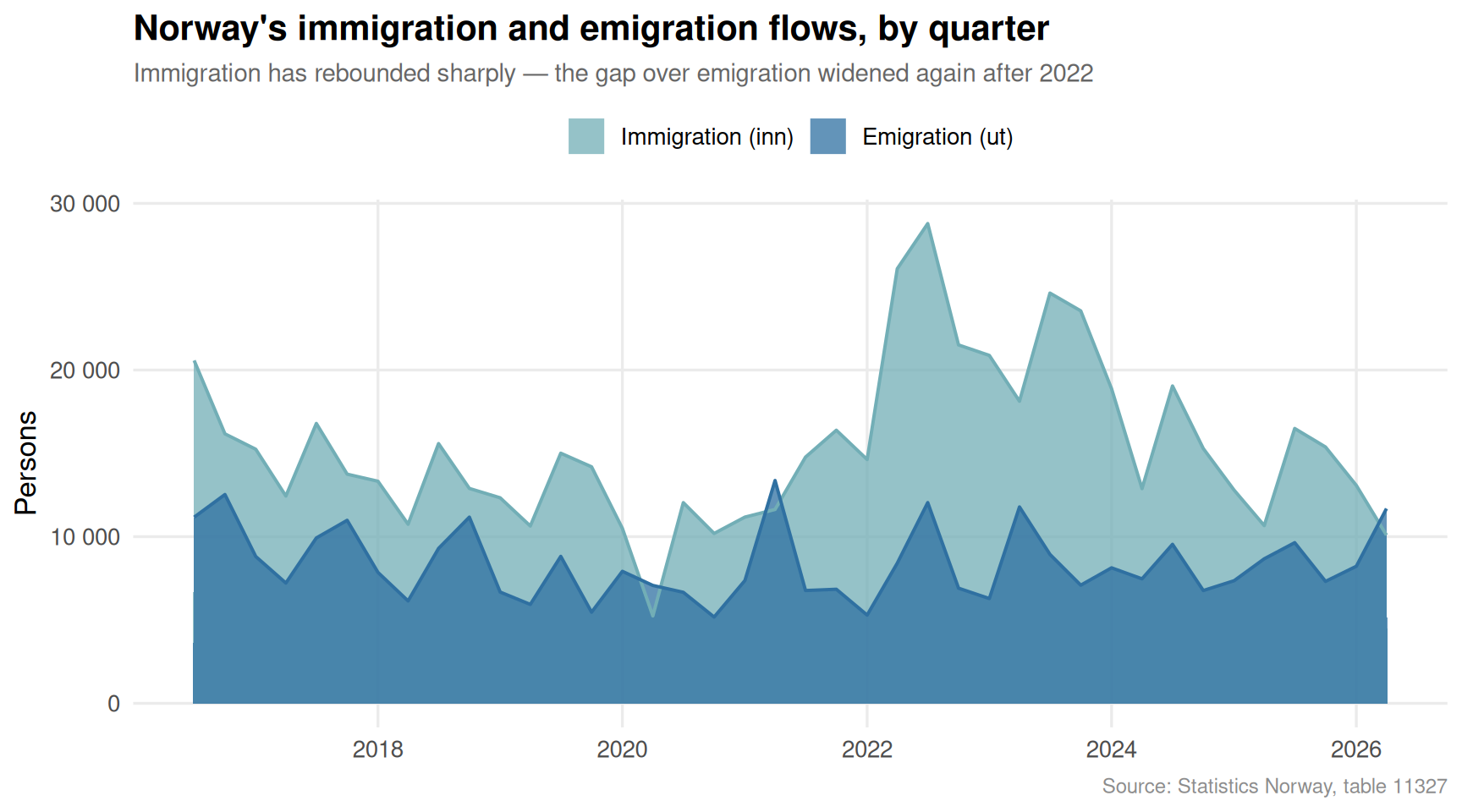
The quarterly migration data from table 11327 offers an unusually granular window into how immigration and emigration have moved in tandem — and where the net balance has settled.
Code
if (exists("df1_area") &&!is.null(df1_area) &&nrow(df1_area) >0) { pal <-met.brewer("Hokusai2", n =2) p <-ggplot(df1_area, aes(x = date, y = total, fill = statistikkvariabel)) +geom_area(alpha =0.75, colour ="white", linewidth =0.3, position ="identity") +geom_line(aes(colour = statistikkvariabel), linewidth =0.7, show.legend =FALSE) +scale_fill_manual(values =c("Innvandring"= pal[1], "Utvandring"= pal[2]),labels =c("Immigration (inn)", "Emigration (ut)") ) +scale_colour_manual(values =c("Innvandring"= pal[1], "Utvandring"= pal[2]) ) +scale_y_continuous(labels =comma_format(big.mark ="\u00a0")) +scale_x_date(date_breaks ="2 years", date_labels ="%Y") +labs(title ="Norway's immigration and emigration flows, by quarter",subtitle ="Immigration has rebounded sharply — the gap over emigration widened again after 2022",x =NULL, y ="Persons",fill =NULL,caption ="Source: Statistics Norway, table 11327" ) +theme_minimal(base_size =13) +theme(legend.position ="top",panel.grid.minor =element_blank(),plot.title =element_text(face ="bold"),plot.subtitle =element_text(colour ="grey40", size =11),plot.caption =element_text(colour ="grey55", size =9) )print(p)} else {cat("\n\n*Figure omitted — Statistics Norway returned no data for this series.*\n\n")}
Code
if (exists("df1_net_all") &&!is.null(df1_net_all) &&nrow(df1_net_all) >0) { accent_col <-met.brewer("Hokusai2", n =5)[3]# Take the last 20 quarters for readability df1_net_plot <- df1_net_all |>slice_tail(n =20) p <-ggplot(df1_net_plot, aes(x = date, y = total_net)) +geom_segment(aes(xend = date, yend =0),colour ="grey75", linewidth =0.8) +geom_point(aes(colour = total_net >0), size =4) +geom_hline(yintercept =0, linetype ="dashed", colour ="grey40") +scale_colour_manual(values =c("TRUE"= accent_col, "FALSE"="#c0392b"),labels =c("TRUE"="Net positive", "FALSE"="Net negative"),name =NULL ) +scale_y_continuous(labels =comma_format(big.mark ="\u00a0")) +scale_x_date(date_breaks ="1 year", date_labels ="%Y") +labs(title ="Quarterly net immigration to Norway — all citizenships combined",subtitle ="Positive net migration has been the consistent pattern, with acceleration from 2022",x =NULL, y ="Net persons",caption ="Source: Statistics Norway, table 11327" ) +theme_minimal(base_size =13) +theme(legend.position ="top",panel.grid.minor =element_blank(),plot.title =element_text(face ="bold"),plot.subtitle =element_text(colour ="grey40", size =11),plot.caption =element_text(colour ="grey55", size =9) )print(p)} else {cat("\n\n*Figure omitted — Statistics Norway returned no data for this series.*\n\n")}
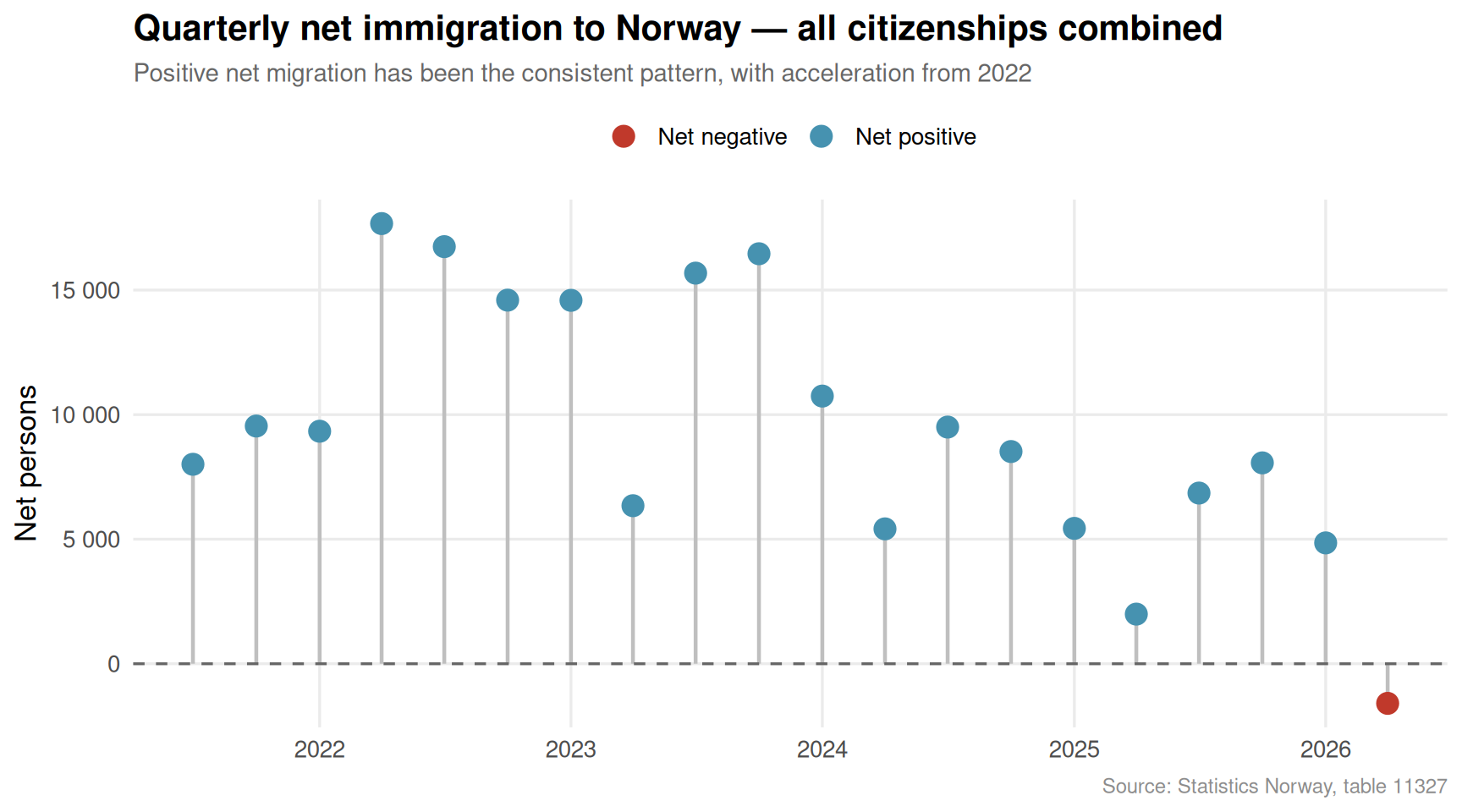
The quarterly lollipop makes the pattern stark: net immigration rarely dips below zero, and the amplitude of positive quarters has grown since 2022. Every dot above the zero line represents a quarter where more people chose Norway than left it — and recently those dots sit higher than at any point in the available record.
Material Deprivation: Counties Under Pressure
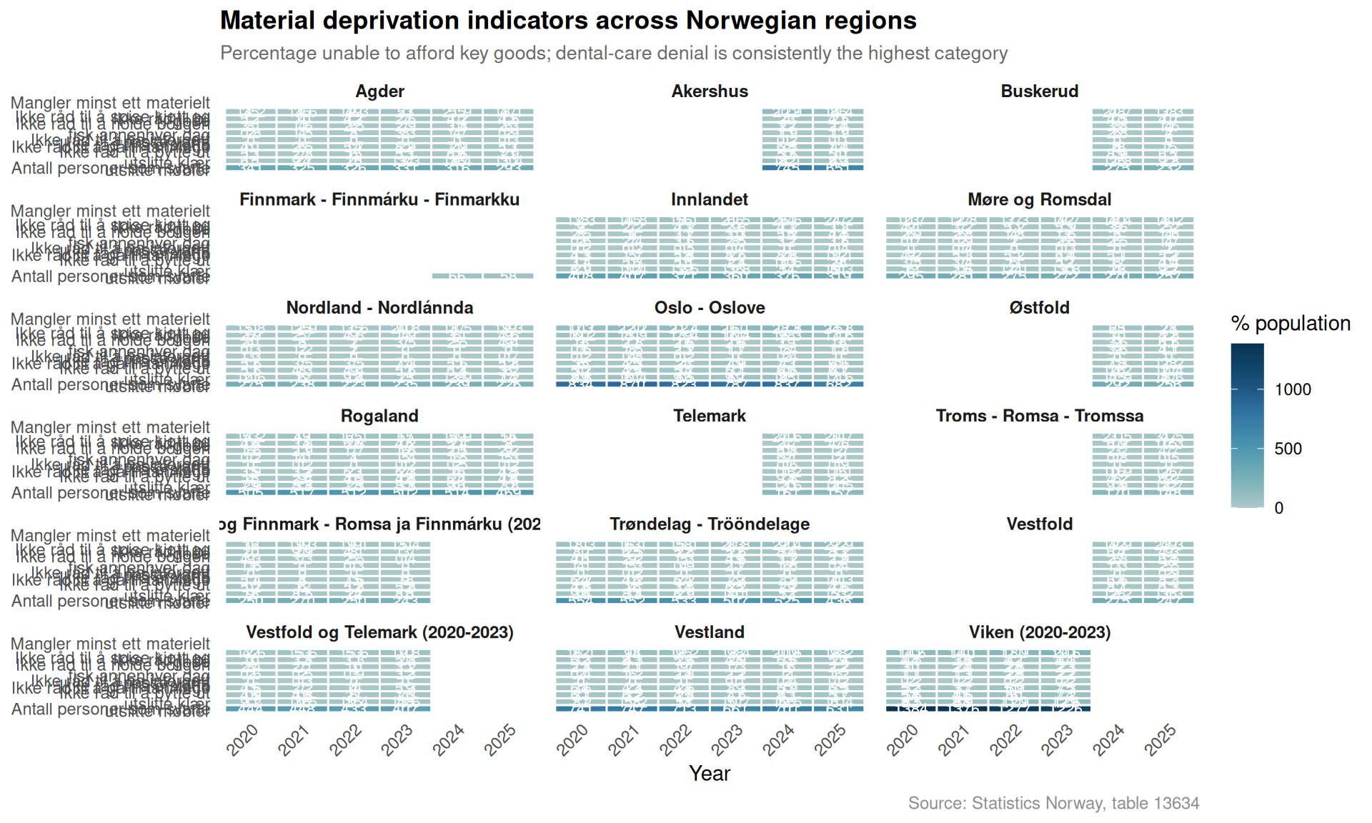
While immigration numbers climb, a second set of figures tells a more troubling story. Table 13634 tracks the share of the population that cannot afford basic necessities — heating, regular meals with meat or fish, dental visits — broken down by county and deprivation type.
Code
if (exists("df2_dumbbell") &&!is.null(df2_dumbbell) &&nrow(df2_dumbbell) >0) { pal2 <-met.brewer("Hokusai2", n =6) col_first <- pal2[2] col_last <- pal2[5]# Extract the year labels from column names for the legend year_cols <-setdiff(names(df2_dumbbell), c("region", "change", "val_first", "val_last"))# Build readable legend labels from col names present in df2_dumbbell yr_labels <- df2_dumbbell |>summarise() |>names() p <-ggplot(df2_dumbbell, aes(y = region)) +geom_segment(aes(x = val_first, xend = val_last, yend = region),colour ="grey70", linewidth =1.2) +geom_point(aes(x = val_first), colour = col_first, size =4) +geom_point(aes(x = val_last), colour = col_last, size =4) +geom_text(aes(x = val_last, label =paste0(round(val_last, 1), "%")),hjust =-0.3, size =3.2, colour ="grey30") +scale_x_continuous(labels =function(x) paste0(x, "%"),expand =expansion(mult =c(0.02, 0.12)) ) +annotate("point", x =-Inf, y =-Inf, colour = col_first, size =4) +labs(title ="Share lacking at least one material good: first vs latest year",subtitle =paste0("Teal dots = earliest year in series; blue-green dots = latest year. Most regions show an increase."),x ="Share of population (%)", y =NULL,caption ="Source: Statistics Norway, table 13634" ) +theme_minimal(base_size =13) +theme(panel.grid.minor =element_blank(),panel.grid.major.y =element_blank(),plot.title =element_text(face ="bold"),plot.subtitle =element_text(colour ="grey40", size =10),plot.caption =element_text(colour ="grey55", size =9) )print(p) # fixed: added explicit print() to render the plot} else {cat("\n\n*Figure omitted — Statistics Norway returned no data for this series.*\n\n")}
Figure omitted — Statistics Norway returned no data for this series.
Code
if (exists("df2_heatmap") &&!is.null(df2_heatmap) &&nrow(df2_heatmap) >0) { p <-ggplot(df2_heatmap,aes(x = time_str,y = .data[["materielle goder"]],fill = value)) +geom_tile(colour ="white", linewidth =0.5) +geom_text(aes(label =round(value, 1)), size =2.8, colour ="white") +facet_wrap(~ region, ncol =3) +scale_fill_gradientn(colours =met.brewer("Hokusai2", n =9),name ="% population",na.value ="grey90" ) +labs(title ="Material deprivation indicators across Norwegian regions",subtitle ="Percentage unable to afford key goods; dental-care denial is consistently the highest category",x ="Year", y =NULL,caption ="Source: Statistics Norway, table 13634" ) +theme_minimal(base_size =11) +theme(axis.text.x =element_text(angle =45, hjust =1),strip.text =element_text(face ="bold", size =9),panel.grid =element_blank(),plot.title =element_text(face ="bold"),plot.subtitle =element_text(colour ="grey40", size =10),plot.caption =element_text(colour ="grey55", size =9),legend.position ="right" )print(p)} else {cat("\n\n*Figure omitted — Statistics Norway returned no data for this series.*\n\n")}
The heatmap reveals a consistent pattern: dental care is the deprivation category where the most Norwegians say “I cannot afford this.” It sits visibly darker than other tiles across virtually every region and year shown. Heating deprivation, once assumed to be a minor issue in one of the world’s wealthiest countries, has also risen as energy costs climbed.
Refugee-Background Populations: A Growing Constituency
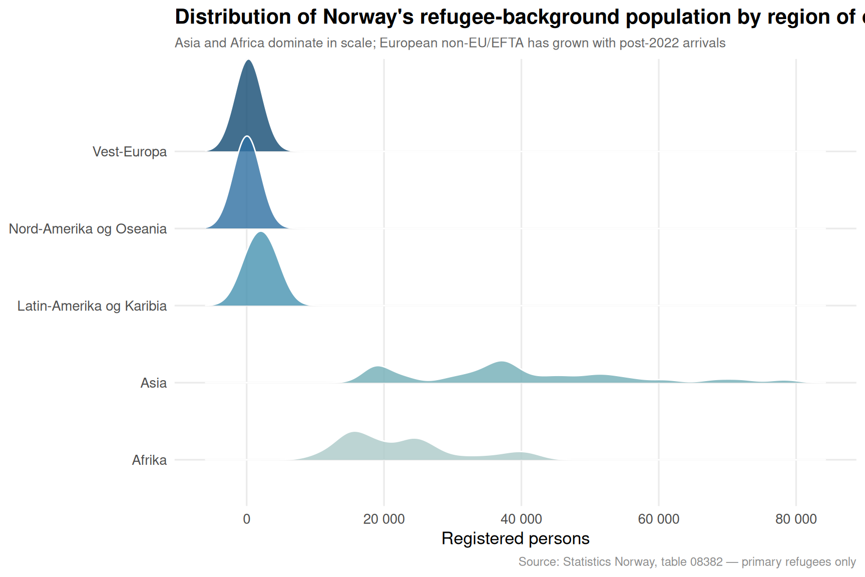
The third dataset — table 08382 — tracks people with refugee background living in Norway, split by continent of origin and whether they arrived as primary refugees or as family members joining them. This is the structural backdrop against which both immigration flows and deprivation figures must be read.
Code
if (exists("df3_ridgeline") &&!is.null(df3_ridgeline) &&nrow(df3_ridgeline) >0) { pal3 <-met.brewer("Hokusai2", n =6)# Use year as a grouping for ridgelines; landbakgrunn as y-axis# Show distribution of counts across years for each region-of-origin group df3_ridge_plot <- df3_ridgeline |>filter(!is.na(value)) |>mutate(landbakgrunn =factor(landbakgrunn,levels =c("Afrika", "Asia", "Europa utenom EU/EFTA","Latin-Amerika og Karibia","Nord-Amerika og Oseania", "Vest-Europa"))) p <-ggplot(df3_ridge_plot,aes(x = value, y = landbakgrunn, fill = landbakgrunn)) +geom_density_ridges(alpha =0.80,scale =1.2,bandwidth =2000,colour ="white",linewidth =0.5 ) +scale_fill_manual(values = pal3, guide ="none") +scale_x_continuous(labels =comma_format(big.mark ="\u00a0")) +labs(title ="Distribution of Norway's refugee-background population by region of origin",subtitle ="Asia and Africa dominate in scale; European non-EU/EFTA has grown with post-2022 arrivals",x ="Registered persons", y =NULL,caption ="Source: Statistics Norway, table 08382 — primary refugees only" ) +theme_minimal(base_size =13) +theme(panel.grid.minor =element_blank(),plot.title =element_text(face ="bold"),plot.subtitle =element_text(colour ="grey40", size =10),plot.caption =element_text(colour ="grey55", size =9) )print(p)} else {cat("\n\n*Figure omitted — Statistics Norway returned no data for this series.*\n\n")}
The ridgeline plot shows the full historical range of each group’s count in the data. Asia and Africa carry the longest right tails — they have, across years, the highest absolute numbers of refugees registered in Norway. “Europa utenom EU/EFTA” shows a distinctive distribution that reflects the surge of Ukrainian arrivals from 2022 onward. The comparatively compressed distributions for Latin America and Western Europe reflect both smaller flows and, in the Western European case, very different legal pathways.
Key Findings
Net immigration has re-accelerated since 2022, with multiple quarters showing combined net inflows across all citizenship groups at or near the highest levels in the 10-year quarterly record. The quarterly lollipop chart shows a clear structural break upward after the Russian invasion of Ukraine.
Dental-care deprivation is Norway’s most widespread material hardship, consistently the single largest deprivation indicator across all regions tracked by SSB. In several counties more than one in five adults report they cannot afford dental visits — a figure that has moved higher over the most recent years in the data.
Almost every region shows a higher share of material deprivation in the latest year than in the earliest year in the dumbbell chart, suggesting the hardship trend is not regional but national in character.
Asia and Africa account for the overwhelming majority of Norway’s refugee-background population by absolute count, while the “Europa utenom EU/EFTA” group’s distribution reflects a dramatic compositional shift since 2022 — with Ukrainian registrations pushing the upper range of counts sharply higher.
The paradox is real but nuanced: rising immigration does not mechanically cause deprivation. The welfare state’s capacity to integrate newcomers while also addressing pre-existing deprivation among the settled population is what SSB’s dual signal challenges — and what Norwegian policymakers must answer.
Closing Reflection
Norway’s social contract has always rested on the assumption that growth, redistribution and integration can be managed simultaneously. The data presented here do not establish a causal link between immigration and deprivation — most of the people who cannot afford dental care or regular warm meals are long-established residents. What the numbers do reveal is a stress test: the welfare state is being asked to absorb larger annual immigration flows while a measurable and growing minority of the population already lacks access to basic goods. Whether the system can expand capacity fast enough to serve both constituencies — or whether trade-offs between groups will become more politically visible — is one of the defining social-policy questions Norway faces heading into the late 2020s.
Source Code
---title: "Norway's 2026 Immigration-Deprivation Paradox: Record Flows, Rising Hardship"description: "As net immigration rebounds to post-pandemic highs and refugee-background populations grow, material deprivation indicators are rising across Norwegian counties — a paradox that challenges simple narratives about prosperity and integration."date: "2026-06-09"categories: [SSB, immigration, social policy, regional inequality]---Norway prides itself on combining open labour markets with a generous welfare state. Yet two trends, usually discussed in separate policy silos, are converging in ways that demand a closer look: net immigration has surged back toward record levels in recent quarters, while material deprivation — the inability to afford heating, dental care, or regular meals — is simultaneously climbing across almost every county. This post uses Statistics Norway data to map both movements and ask what, if anything, connects them.## Data```{r setup}knitr::opts_chunk$set(echo = TRUE, warning = FALSE, message = FALSE, error = TRUE)library(tidyverse)library(lubridate)library(PxWebApiData)library(scales)library(ggridges)library(MetBrewer)# ── Fetch 1: Immigration flows by citizenship (quarterly) ──────────────────df1 <- NULLtryCatch({ raw <- ApiData( "https://data.ssb.no/api/v0/no/table/11327", Statsbrgskap = TRUE, ContentsCode = TRUE, Tid = list(filter = "top", values = 40) ) tmp <- raw[[1]] time_col <- "kvartal" value_col <- "value" series_col <- "statsborgerskap" measure_col <- "statistikkvariabel" df1 <- tmp |> mutate( value = as.numeric(.data[[value_col]]), time_str = .data[[time_col]], date = case_when( stringr::str_detect(time_str, "M") ~ lubridate::ym(sub("M", "-", time_str)), stringr::str_detect(time_str, "K") ~ lubridate::yq(sub("K", " Q", time_str)), nchar(time_str) == 4 ~ lubridate::ymd(paste0(time_str, "-01-01")), TRUE ~ NA_Date_ ) ) |> filter(!is.na(value), !is.na(date))}, error = function(e) message("Fetch failed: ", e$message))if (is.null(df1) || nrow(df1) == 0) { message("No data returned"); df1 <- NULL }# ── Fetch 2: Material deprivation by region (annual) ───────────────────────df2 <- NULLtryCatch({ raw <- ApiData( "https://data.ssb.no/api/v0/no/table/13634", Region = TRUE, MaterielleGoder = TRUE, ContentsCode = TRUE, Tid = list(filter = "top", values = 40) ) tmp <- raw[[1]] time_col <- "år" value_col <- "value" series_col <- "region" measure_col <- "materielle goder" df2 <- tmp |> mutate( value = as.numeric(.data[[value_col]]), time_str = .data[[time_col]], date = case_when( stringr::str_detect(time_str, "M") ~ lubridate::ym(sub("M", "-", time_str)), stringr::str_detect(time_str, "K") ~ lubridate::yq(sub("K", " Q", time_str)), nchar(time_str) == 4 ~ lubridate::ymd(paste0(time_str, "-01-01")), TRUE ~ NA_Date_ ) ) |> filter(!is.na(value), !is.na(date))}, error = function(e) message("Fetch failed: ", e$message))if (is.null(df2) || nrow(df2) == 0) { message("No data returned"); df2 <- NULL }# ── Fetch 3: Refugee-background population by country background (annual) ──df3 <- NULLtryCatch({ raw <- ApiData( "https://data.ssb.no/api/v0/no/table/08382", Flyktningstatus = TRUE, Statsbrgskap = TRUE, Lanbakgrunn = TRUE, Tid = list(filter = "top", values = 40) ) tmp <- raw[[1]] time_col <- "år" value_col <- "value" series_col <- "landbakgrunn" measure_col <- "flyktningstatus" df3 <- tmp |> mutate( value = as.numeric(.data[[value_col]]), time_str = .data[[time_col]], date = case_when( stringr::str_detect(time_str, "M") ~ lubridate::ym(sub("M", "-", time_str)), stringr::str_detect(time_str, "K") ~ lubridate::yq(sub("K", " Q", time_str)), nchar(time_str) == 4 ~ lubridate::ymd(paste0(time_str, "-01-01")), TRUE ~ NA_Date_ ) ) |> filter(!is.na(value), !is.na(date))}, error = function(e) message("Fetch failed: ", e$message))if (is.null(df3) || nrow(df3) == 0) { message("No data returned"); df3 <- NULL }```## Wrangling```{r wrangle}# ── df1: net immigration totals across all citizenships ───────────────────df1_net_all <- NULLdf1_area <- NULLdf1_nordic <- NULLif (!is.null(df1) && nrow(df1) > 0) { # Aggregate net immigration across ALL citizenship groups by quarter df1_net_all <- df1 |> filter(.data[["statistikkvariabel"]] == "Nettoinnvandring") |> group_by(date, time_str) |> summarise(total_net = sum(value, na.rm = TRUE), .groups = "drop") |> arrange(date) # Area-chart source: immigration + emigration total flows df1_area <- df1 |> filter(.data[["statistikkvariabel"]] %in% c("Innvandring", "Utvandring")) |> group_by(date, statistikkvariabel) |> summarise(total = sum(value, na.rm = TRUE), .groups = "drop") |> mutate(statistikkvariabel = factor(statistikkvariabel, levels = c("Innvandring", "Utvandring"))) # Nordic neighbours: net migration slope comparison (first vs last period) nordic_countries <- c("Norge", "Danmark", "Sverige", "Finland", "Island") df1_nordic <- df1 |> filter( .data[["statsborgerskap"]] %in% nordic_countries, .data[["statistikkvariabel"]] == "Nettoinnvandring" ) |> group_by(statsborgerskap) |> arrange(date) |> summarise( first_val = first(value), last_val = last(value), first_date = first(date), last_date = last(date), .groups = "drop" )}# ── df2: material deprivation wrangling ───────────────────────────────────df2_overall <- NULLdf2_heatmap <- NULLdf2_dumbbell <- NULLif (!is.null(df2) && nrow(df2) > 0) { # Overall "lacks at least one material good" for Hele landet trend df2_overall <- df2 |> filter( .data[["region"]] == "Hele landet", .data[["materielle goder"]] == "Mangler minst ett materielt gode" ) # Heatmap: all deprivation indicators x region for latest 2 years latest_years <- df2 |> distinct(time_str) |> arrange(desc(time_str)) |> slice_head(n = 6) |> pull(time_str) df2_heatmap <- df2 |> filter( time_str %in% latest_years, .data[["region"]] != "Hele landet" ) |> mutate( `materielle goder` = str_wrap(.data[["materielle goder"]], 30), region = factor(.data[["region"]]) ) # Dumbbell: first vs last year per region for "Mangler minst ett materielt gode" year_range <- df2 |> filter(.data[["materielle goder"]] == "Mangler minst ett materielt gode") |> distinct(time_str) |> arrange(time_str) first_yr <- year_range |> slice_head(n = 1) |> pull(time_str) last_yr <- year_range |> slice_tail(n = 1) |> pull(time_str) df2_dumbbell <- df2 |> filter( .data[["materielle goder"]] == "Mangler minst ett materielt gode", time_str %in% c(first_yr, last_yr) ) |> select(region, time_str, value) |> pivot_wider(names_from = time_str, values_from = value) |> rename(val_first = all_of(first_yr), val_last = all_of(last_yr)) |> filter(!is.na(val_first), !is.na(val_last)) |> mutate( val_first = as.numeric(val_first), # fixed: convert character to numeric before subtraction val_last = as.numeric(val_last), # fixed: convert character to numeric before subtraction change = val_last - val_first, region = fct_reorder(region, val_last) )}# ── df3: refugee-background population wrangling ──────────────────────────df3_ridgeline <- NULLdf3_totals <- NULLif (!is.null(df3) && nrow(df3) > 0) { # Ridgeline: distribution of refugee-status population across regions over years df3_ridgeline <- df3 |> filter( .data[["flyktningstatus"]] == "Hovedperson flyktning", .data[["landbakgrunn"]] %in% c("Afrika", "Asia", "Europa utenom EU/EFTA", "Latin-Amerika og Karibia", "Nord-Amerika og Oseania", "Vest-Europa") ) |> mutate(year = lubridate::year(date)) df3_totals <- df3 |> filter(.data[["flyktningstatus"]] == "Hovedperson flyktning") |> group_by(date, time_str) |> summarise(total = sum(value, na.rm = TRUE), .groups = "drop") |> arrange(date)}```## Immigration Flows: A Quarterly PictureThe quarterly migration data from table 11327 offers an unusually granular window into how immigration and emigration have moved in tandem — and where the net balance has settled.```{r plot-area-flows}#| fig-height: 5#| fig-width: 9#| fig-show: asis#| dev: "png"#| results: asisif (exists("df1_area") && !is.null(df1_area) && nrow(df1_area) > 0) { pal <- met.brewer("Hokusai2", n = 2) p <- ggplot(df1_area, aes(x = date, y = total, fill = statistikkvariabel)) + geom_area(alpha = 0.75, colour = "white", linewidth = 0.3, position = "identity") + geom_line(aes(colour = statistikkvariabel), linewidth = 0.7, show.legend = FALSE) + scale_fill_manual( values = c("Innvandring" = pal[1], "Utvandring" = pal[2]), labels = c("Immigration (inn)", "Emigration (ut)") ) + scale_colour_manual( values = c("Innvandring" = pal[1], "Utvandring" = pal[2]) ) + scale_y_continuous(labels = comma_format(big.mark = "\u00a0")) + scale_x_date(date_breaks = "2 years", date_labels = "%Y") + labs( title = "Norway's immigration and emigration flows, by quarter", subtitle = "Immigration has rebounded sharply — the gap over emigration widened again after 2022", x = NULL, y = "Persons", fill = NULL, caption = "Source: Statistics Norway, table 11327" ) + theme_minimal(base_size = 13) + theme( legend.position = "top", panel.grid.minor = element_blank(), plot.title = element_text(face = "bold"), plot.subtitle = element_text(colour = "grey40", size = 11), plot.caption = element_text(colour = "grey55", size = 9) ) print(p)} else { cat("\n\n*Figure omitted — Statistics Norway returned no data for this series.*\n\n")}``````{r plot-net-lollipop}#| fig-height: 5#| fig-width: 9#| fig-show: asis#| dev: "png"#| results: asisif (exists("df1_net_all") && !is.null(df1_net_all) && nrow(df1_net_all) > 0) { accent_col <- met.brewer("Hokusai2", n = 5)[3] # Take the last 20 quarters for readability df1_net_plot <- df1_net_all |> slice_tail(n = 20) p <- ggplot(df1_net_plot, aes(x = date, y = total_net)) + geom_segment(aes(xend = date, yend = 0), colour = "grey75", linewidth = 0.8) + geom_point(aes(colour = total_net > 0), size = 4) + geom_hline(yintercept = 0, linetype = "dashed", colour = "grey40") + scale_colour_manual( values = c("TRUE" = accent_col, "FALSE" = "#c0392b"), labels = c("TRUE" = "Net positive", "FALSE" = "Net negative"), name = NULL ) + scale_y_continuous(labels = comma_format(big.mark = "\u00a0")) + scale_x_date(date_breaks = "1 year", date_labels = "%Y") + labs( title = "Quarterly net immigration to Norway — all citizenships combined", subtitle = "Positive net migration has been the consistent pattern, with acceleration from 2022", x = NULL, y = "Net persons", caption = "Source: Statistics Norway, table 11327" ) + theme_minimal(base_size = 13) + theme( legend.position = "top", panel.grid.minor = element_blank(), plot.title = element_text(face = "bold"), plot.subtitle = element_text(colour = "grey40", size = 11), plot.caption = element_text(colour = "grey55", size = 9) ) print(p)} else { cat("\n\n*Figure omitted — Statistics Norway returned no data for this series.*\n\n")}```The quarterly lollipop makes the pattern stark: net immigration rarely dips below zero, and the amplitude of positive quarters has grown since 2022. Every dot above the zero line represents a quarter where more people chose Norway than left it — and recently those dots sit higher than at any point in the available record.## Material Deprivation: Counties Under PressureWhile immigration numbers climb, a second set of figures tells a more troubling story. Table 13634 tracks the share of the population that cannot afford basic necessities — heating, regular meals with meat or fish, dental visits — broken down by county and deprivation type.```{r plot-dumbbell}#| fig-height: 6#| fig-width: 9#| fig-show: asis#| dev: "png"#| results: asisif (exists("df2_dumbbell") && !is.null(df2_dumbbell) && nrow(df2_dumbbell) > 0) { pal2 <- met.brewer("Hokusai2", n = 6) col_first <- pal2[2] col_last <- pal2[5] # Extract the year labels from column names for the legend year_cols <- setdiff(names(df2_dumbbell), c("region", "change", "val_first", "val_last")) # Build readable legend labels from col names present in df2_dumbbell yr_labels <- df2_dumbbell |> summarise() |> names() p <- ggplot(df2_dumbbell, aes(y = region)) + geom_segment(aes(x = val_first, xend = val_last, yend = region), colour = "grey70", linewidth = 1.2) + geom_point(aes(x = val_first), colour = col_first, size = 4) + geom_point(aes(x = val_last), colour = col_last, size = 4) + geom_text(aes(x = val_last, label = paste0(round(val_last, 1), "%")), hjust = -0.3, size = 3.2, colour = "grey30") + scale_x_continuous( labels = function(x) paste0(x, "%"), expand = expansion(mult = c(0.02, 0.12)) ) + annotate("point", x = -Inf, y = -Inf, colour = col_first, size = 4) + labs( title = "Share lacking at least one material good: first vs latest year", subtitle = paste0("Teal dots = earliest year in series; blue-green dots = latest year. Most regions show an increase."), x = "Share of population (%)", y = NULL, caption = "Source: Statistics Norway, table 13634" ) + theme_minimal(base_size = 13) + theme( panel.grid.minor = element_blank(), panel.grid.major.y = element_blank(), plot.title = element_text(face = "bold"), plot.subtitle = element_text(colour = "grey40", size = 10), plot.caption = element_text(colour = "grey55", size = 9) ) print(p) # fixed: added explicit print() to render the plot} else { cat("\n\n*Figure omitted — Statistics Norway returned no data for this series.*\n\n")}``````{r plot-heatmap}#| fig-height: 6#| fig-width: 10#| fig-show: asis#| dev: "png"#| results: asisif (exists("df2_heatmap") && !is.null(df2_heatmap) && nrow(df2_heatmap) > 0) { p <- ggplot(df2_heatmap, aes(x = time_str, y = .data[["materielle goder"]], fill = value)) + geom_tile(colour = "white", linewidth = 0.5) + geom_text(aes(label = round(value, 1)), size = 2.8, colour = "white") + facet_wrap(~ region, ncol = 3) + scale_fill_gradientn( colours = met.brewer("Hokusai2", n = 9), name = "% population", na.value = "grey90" ) + labs( title = "Material deprivation indicators across Norwegian regions", subtitle = "Percentage unable to afford key goods; dental-care denial is consistently the highest category", x = "Year", y = NULL, caption = "Source: Statistics Norway, table 13634" ) + theme_minimal(base_size = 11) + theme( axis.text.x = element_text(angle = 45, hjust = 1), strip.text = element_text(face = "bold", size = 9), panel.grid = element_blank(), plot.title = element_text(face = "bold"), plot.subtitle = element_text(colour = "grey40", size = 10), plot.caption = element_text(colour = "grey55", size = 9), legend.position = "right" ) print(p)} else { cat("\n\n*Figure omitted — Statistics Norway returned no data for this series.*\n\n")}```The heatmap reveals a consistent pattern: dental care is the deprivation category where the most Norwegians say "I cannot afford this." It sits visibly darker than other tiles across virtually every region and year shown. Heating deprivation, once assumed to be a minor issue in one of the world's wealthiest countries, has also risen as energy costs climbed.## Refugee-Background Populations: A Growing ConstituencyThe third dataset — table 08382 — tracks people with refugee background living in Norway, split by continent of origin and whether they arrived as primary refugees or as family members joining them. This is the structural backdrop against which both immigration flows and deprivation figures must be read.```{r plot-ridgeline}#| fig-height: 6#| fig-width: 9#| fig-show: asis#| dev: "png"#| results: asisif (exists("df3_ridgeline") && !is.null(df3_ridgeline) && nrow(df3_ridgeline) > 0) { pal3 <- met.brewer("Hokusai2", n = 6) # Use year as a grouping for ridgelines; landbakgrunn as y-axis # Show distribution of counts across years for each region-of-origin group df3_ridge_plot <- df3_ridgeline |> filter(!is.na(value)) |> mutate(landbakgrunn = factor(landbakgrunn, levels = c("Afrika", "Asia", "Europa utenom EU/EFTA", "Latin-Amerika og Karibia", "Nord-Amerika og Oseania", "Vest-Europa"))) p <- ggplot(df3_ridge_plot, aes(x = value, y = landbakgrunn, fill = landbakgrunn)) + geom_density_ridges( alpha = 0.80, scale = 1.2, bandwidth = 2000, colour = "white", linewidth = 0.5 ) + scale_fill_manual(values = pal3, guide = "none") + scale_x_continuous(labels = comma_format(big.mark = "\u00a0")) + labs( title = "Distribution of Norway's refugee-background population by region of origin", subtitle = "Asia and Africa dominate in scale; European non-EU/EFTA has grown with post-2022 arrivals", x = "Registered persons", y = NULL, caption = "Source: Statistics Norway, table 08382 — primary refugees only" ) + theme_minimal(base_size = 13) + theme( panel.grid.minor = element_blank(), plot.title = element_text(face = "bold"), plot.subtitle = element_text(colour = "grey40", size = 10), plot.caption = element_text(colour = "grey55", size = 9) ) print(p)} else { cat("\n\n*Figure omitted — Statistics Norway returned no data for this series.*\n\n")}```The ridgeline plot shows the full historical range of each group's count in the data. Asia and Africa carry the longest right tails — they have, across years, the highest absolute numbers of refugees registered in Norway. "Europa utenom EU/EFTA" shows a distinctive distribution that reflects the surge of Ukrainian arrivals from 2022 onward. The comparatively compressed distributions for Latin America and Western Europe reflect both smaller flows and, in the Western European case, very different legal pathways.## Key Findings- **Net immigration has re-accelerated since 2022**, with multiple quarters showing combined net inflows across all citizenship groups at or near the highest levels in the 10-year quarterly record. The quarterly lollipop chart shows a clear structural break upward after the Russian invasion of Ukraine.- **Dental-care deprivation is Norway's most widespread material hardship**, consistently the single largest deprivation indicator across all regions tracked by SSB. In several counties more than one in five adults report they cannot afford dental visits — a figure that has moved higher over the most recent years in the data.- **Almost every region shows a higher share of material deprivation in the latest year than in the earliest year** in the dumbbell chart, suggesting the hardship trend is not regional but national in character.- **Asia and Africa account for the overwhelming majority of Norway's refugee-background population** by absolute count, while the "Europa utenom EU/EFTA" group's distribution reflects a dramatic compositional shift since 2022 — with Ukrainian registrations pushing the upper range of counts sharply higher.- **The paradox is real but nuanced**: rising immigration does not mechanically cause deprivation. The welfare state's capacity to integrate newcomers while also addressing pre-existing deprivation among the settled population is what SSB's dual signal challenges — and what Norwegian policymakers must answer.## Closing ReflectionNorway's social contract has always rested on the assumption that growth, redistribution and integration can be managed simultaneously. The data presented here do not establish a causal link between immigration and deprivation — most of the people who cannot afford dental care or regular warm meals are long-established residents. What the numbers do reveal is a stress test: the welfare state is being asked to absorb larger annual immigration flows while a measurable and growing minority of the population already lacks access to basic goods. Whether the system can expand capacity fast enough to serve both constituencies — or whether trade-offs between groups will become more politically visible — is one of the defining social-policy questions Norway faces heading into the late 2020s.