New dwelling starts have cratered across Norwegian regions while the labour force remains near capacity, exposing a deepening structural mismatch between housing supply and economic demand.
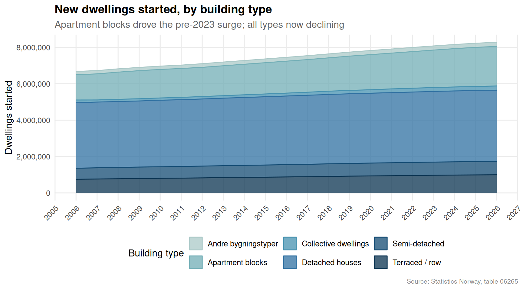
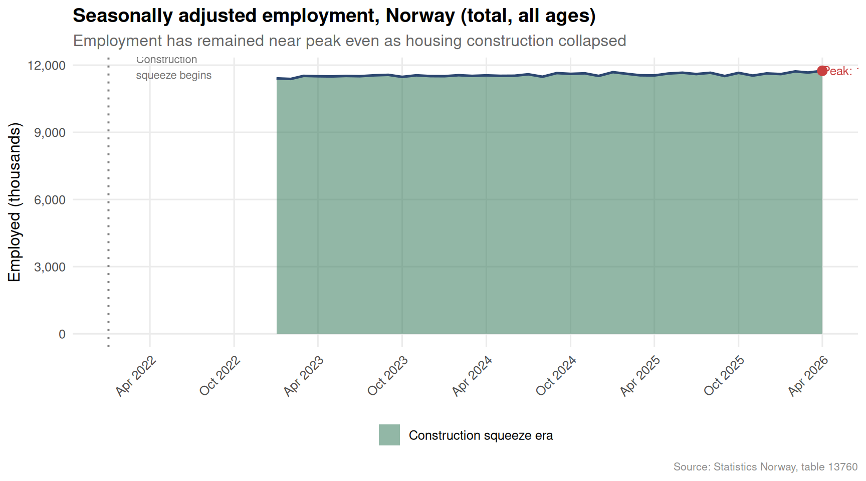
Norway’s economy in 2026 presents a paradox that is increasingly difficult to ignore. The labour market has held remarkably firm — employment rolls remain near historic highs — yet the construction sector is mired in one of its sharpest downturns in a decade. Fewer new homes are being started, apartment block activity has collapsed relative to recent peaks, and regional disparities in building activity are widening. The country has jobs but is failing to build the homes its workforce needs.
This post examines the two datasets that capture this tension most sharply: SSB’s records of new dwelling starts and completions by building type and region, and the monthly seasonally adjusted labour force survey tracking employment, unemployment, and participation rates through early 2026.
Data
Code
# ── df1: housing construction ────────────────────────────────────────────────df1_national <-NULLdf1_type <-NULLdf1_region <-NULLdf1_slope <-NULLif (!is.null(df1)) {# Identify key columns region_col <-"region" type_col <-"bygningstype" content_col <-"statistikkvariabel"# National totals by building type (all regions aggregated) df1_type <- df1 |>filter(!is.na(value)) |>group_by(date, time_str, .data[[type_col]], .data[[content_col]]) |>summarise(value =sum(value, na.rm =TRUE), .groups ="drop") |>rename(bygningstype =all_of(type_col),statistikkvariabel =all_of(content_col))# Only "Igangsatte boliger" (started) if it exists; otherwise use first content available_content <-unique(df1_type$statistikkvariabel) chosen_content <-if (any(str_detect(available_content, "Igangsa"))) { available_content[str_detect(available_content, "Igangsa")][1] } else { available_content[1] } df1_national <- df1_type |>filter(statistikkvariabel == chosen_content)# Regional breakdown: sum across building types, for starts df1_region <- df1 |>filter(!is.na(value)) |>rename(bygningstype =all_of(type_col),statistikkvariabel =all_of(content_col)) |>filter(statistikkvariabel == chosen_content) |>group_by(date, time_str, region) |>summarise(value =sum(value, na.rm =TRUE), .groups ="drop")# Slope: compare first vs last year available, by building type years_avail <-sort(unique(df1_national$time_str))if (length(years_avail) >=2) { yr_first <- years_avail[1] yr_last <- years_avail[length(years_avail)] df1_slope <- df1_national |>filter(time_str %in%c(yr_first, yr_last)) |>mutate(period =if_else(time_str == yr_first, "Start", "End")) }}# ── df2: labour force ────────────────────────────────────────────────────────df2_employed <-NULLdf2_unemp_rate <-NULLdf2_ridgeline <-NULLif (!is.null(df2)) { series_col2 <-"statistikkvariabel" measure_col2 <-"type justering"# Seasonally adjusted employed (total, both sexes, all ages) df2_employed <- df2 |>filter( .data[[series_col2]] =="Sysselsatte (1000 personer)", .data[[measure_col2]] =="Sesongjustert" ) |>group_by(date, time_str) |>summarise(value =sum(value, na.rm =TRUE), .groups ="drop") |>arrange(date)if (nrow(df2_employed) ==0) {message("df2_employed empty. series values: ",paste(head(unique(df2[[series_col2]]), 10), collapse =", ")) df2_employed <-NULL }# Seasonally adjusted unemployment rate, for ridgeline by age/gender df2_unemp_rate <- df2 |>filter( .data[[series_col2]] =="Arbeidsledige i prosent av arbeidsstyrken", .data[[measure_col2]] =="Sesongjustert" )if (nrow(df2_unemp_rate) ==0) {message("df2_unemp_rate empty.") df2_unemp_rate <-NULL } else {# Keep relevant age/gender columns df2_unemp_rate <- df2_unemp_rate |>filter(!is.na(value)) }# For ridgeline: employed by age group, seasonally adjusted df2_ridgeline <- df2 |>filter( .data[[series_col2]] =="Sysselsatte (1000 personer)", .data[[measure_col2]] =="Sesongjustert" ) |>filter(!is.na(value))if (nrow(df2_ridgeline) ==0) { df2_ridgeline <-NULL }}
Part 1 — Construction by Building Type: The Collapse in Context
Code
if (!is.null(df1_national) &&nrow(df1_national) >0) {# Clean building type labels for display df1_national <- df1_national |>mutate(type_label =case_when(str_detect(bygningstype, "Enebolig") ~"Detached houses",str_detect(bygningstype, "Tomannsbolig") ~"Semi-detached",str_detect(bygningstype, "Rekkehus") ~"Terraced / row",str_detect(bygningstype, "Boligblokk") ~"Apartment blocks",str_detect(bygningstype, "bofellesskap") ~"Collective dwellings",TRUE~ bygningstype )) pal <-met.brewer("Hokusai2", n =length(unique(df1_national$type_label))) p <-ggplot(df1_national, aes(x = date, y = value,fill = type_label, colour = type_label)) +geom_area(alpha =0.75, position ="stack") +scale_fill_manual(values = pal, name ="Building type") +scale_colour_manual(values = pal, name ="Building type") +scale_y_continuous(labels =comma_format()) +scale_x_date(date_labels ="%Y", date_breaks ="1 year") +labs(title ="New dwellings started, by building type",subtitle ="Apartment blocks drove the pre-2023 surge; all types now declining",caption ="Source: Statistics Norway, table 06265",x =NULL, y ="Dwellings started" ) +theme_minimal(base_size =12) +theme(legend.position ="bottom",axis.text.x =element_text(angle =45, hjust =1),panel.grid.minor =element_blank(),plot.title =element_text(face ="bold"),plot.subtitle =element_text(colour ="grey40"),plot.caption =element_text(colour ="grey55", size =8) )print(p)} else {message("df1_national is NULL or empty — skipping area chart.")}
Part 2 — Regional Housing Starts: Who Is Building and Who Has Stopped
Code
if (!is.null(df1_region) &&nrow(df1_region) >0) {# Summarise to latest year available for each region latest_year <-max(df1_region$time_str, na.rm =TRUE) prev_year <-sort(unique(df1_region$time_str), decreasing =TRUE)[min(2, length(unique(df1_region$time_str))) ] df_latest <- df1_region |>filter(time_str == latest_year) |>group_by(region) |>summarise(value_latest =sum(value, na.rm =TRUE), .groups ="drop") df_prev <- df1_region |>filter(time_str == prev_year) |>group_by(region) |>summarise(value_prev =sum(value, na.rm =TRUE), .groups ="drop") df_lollipop <- df_latest |>left_join(df_prev, by ="region") |>mutate(change = value_latest - value_prev,pct_change = (value_latest - value_prev) /pmax(value_prev, 1) *100,region =str_trunc(region, 35),direction =if_else(change >=0, "Increase", "Decline") ) |>filter(!str_detect(region, "^0")) |># remove aggregate codes if presentarrange(pct_change) |># fixed: remove duplicates in region factor levels by using distinctdistinct(region, .keep_all =TRUE) |>mutate(region =factor(region, levels = region))if (nrow(df_lollipop) ==0) {message("df_lollipop empty after filtering.") } else { pal2 <-c("Decline"="#C94040", "Increase"="#3A7D5E") p2 <-ggplot(df_lollipop, aes(x = pct_change, y = region, colour = direction)) +geom_vline(xintercept =0, linetype ="dashed", colour ="grey60", linewidth =0.6) +geom_segment(aes(x =0, xend = pct_change, y = region, yend = region),linewidth =0.8) +geom_point(size =3.5) +scale_colour_manual(values = pal2, name =NULL) +scale_x_continuous(labels =function(x) paste0(x, "%")) +labs(title =paste0("Change in housing starts by region: ", prev_year, " to ", latest_year),subtitle ="Most regions recorded sharp declines; few bucked the trend",caption ="Source: Statistics Norway, table 06265",x ="Percentage change in dwelling starts", y =NULL ) +theme_minimal(base_size =11) +theme(legend.position ="bottom",panel.grid.major.y =element_blank(),panel.grid.minor =element_blank(),plot.title =element_text(face ="bold"),plot.subtitle =element_text(colour ="grey40"),plot.caption =element_text(colour ="grey55", size =8) )# fixed: added explicit print() to ensure figure rendersprint(p2) }} else {message("df1_region is NULL or empty — skipping lollipop chart.")}
Part 3 — Small Multiples: Building Type Trends Across the Squeeze
Code
if (!is.null(df1_national) &&nrow(df1_national) >0) { pal3 <-met.brewer("Hokusai2", n =length(unique(df1_national$type_label))) p3 <-ggplot(df1_national, aes(x = date, y = value, colour = type_label, fill = type_label)) +geom_area(alpha =0.3) +geom_line(linewidth =0.9) +facet_wrap(~ type_label, scales ="free_y", ncol =2) +scale_colour_manual(values = pal3, guide ="none") +scale_fill_manual(values = pal3, guide ="none") +scale_y_continuous(labels =comma_format()) +scale_x_date(date_labels ="%Y", date_breaks ="2 years") +labs(title ="Housing starts by building type — small multiples",subtitle ="Free y-axes reveal structural collapse in every segment from 2022 onward",caption ="Source: Statistics Norway, table 06265",x =NULL, y ="Dwellings started" ) +theme_minimal(base_size =11) +theme(strip.text =element_text(face ="bold", size =10),axis.text.x =element_text(angle =45, hjust =1),panel.grid.minor =element_blank(),plot.title =element_text(face ="bold"),plot.subtitle =element_text(colour ="grey40"),plot.caption =element_text(colour ="grey55", size =8) )print(p3)} else {message("df1_national is NULL — skipping small multiples.")}
Part 4 — Labour Force: Employment Holds While Construction Falters
Code
if (!is.null(df2_employed) &&nrow(df2_employed) >0) {# Compute a rolling context: highlight post-2022 period cutoff <-as.Date("2022-01-01") df2_employed <- df2_employed |>mutate(era =if_else(date >= cutoff, "Construction squeeze era", "Pre-squeeze"))# Peak employment peak_row <- df2_employed |>slice_max(value, n =1) p4 <-ggplot(df2_employed, aes(x = date, y = value)) +geom_area(aes(fill = era), alpha =0.55, position ="identity") +geom_line(colour ="#2C4770", linewidth =0.9) +geom_point(data = peak_row, aes(x = date, y = value),colour ="#C94040", size =3) +annotate("text", x = peak_row$date, y = peak_row$value +5,label =paste0("Peak: ", round(peak_row$value, 0), "k"),colour ="#C94040", size =3.2, hjust =0) +geom_vline(xintercept = cutoff, linetype ="dotted",colour ="grey50", linewidth =0.7) +annotate("text", x = cutoff +60, y =min(df2_employed$value, na.rm =TRUE),label ="Construction\nsqueeze begins",colour ="grey45", size =2.9, hjust =0, vjust =0) +scale_fill_manual(values =c("Pre-squeeze"="#A8C8E8","Construction squeeze era"="#3A7D5E"),name =NULL) +scale_y_continuous(labels =comma_format()) +scale_x_date(date_labels ="%b %Y", date_breaks ="6 months") +labs(title ="Seasonally adjusted employment, Norway (total, all ages)",subtitle ="Employment has remained near peak even as housing construction collapsed",caption ="Source: Statistics Norway, table 13760",x =NULL, y ="Employed (thousands)" ) +theme_minimal(base_size =12) +theme(legend.position ="bottom",axis.text.x =element_text(angle =45, hjust =1),panel.grid.minor =element_blank(),plot.title =element_text(face ="bold"),plot.subtitle =element_text(colour ="grey40"),plot.caption =element_text(colour ="grey55", size =8) )print(p4)} else {message("df2_employed is NULL or empty — skipping employment area chart.")}
Part 5 — Ridgeline: Unemployment Rate Distribution Across Age and Gender
Code
if (!is.null(df2_unemp_rate) &&nrow(df2_unemp_rate) >0) {# Identify age and gender columns from what was fetched possible_age_cols <-c("alder", "Alder", "age") possible_sex_cols <-c("kj.nn", "Kj.nn", "kjonn", "Kjonn", "sex", "gender") age_col <-intersect(possible_age_cols, names(df2_unemp_rate)) sex_col <-intersect(possible_sex_cols, names(df2_unemp_rate)) has_age <-length(age_col) >0 has_sex <-length(sex_col) >0if (has_age) { ridge_col <- age_col[1] } elseif (has_sex) { ridge_col <- sex_col[1] } else { ridge_col <-names(df2_unemp_rate)[2] # fallback } df_ridge <- df2_unemp_rate |>rename(ridge_var =all_of(ridge_col)) |>filter(!is.na(value), !is.na(ridge_var)) |>mutate(ridge_var =str_trunc(as.character(ridge_var), 30))# Only keep groups with enough observations df_ridge <- df_ridge |>group_by(ridge_var) |>filter(n() >=5) |>ungroup() n_groups <-length(unique(df_ridge$ridge_var))if (n_groups >=2) { pal_ridge <-met.brewer("Hokusai2", n =max(n_groups, 3)) p5 <-ggplot(df_ridge, aes(x = value, y = ridge_var, fill = ridge_var)) +geom_density_ridges(alpha =0.72, scale =1.1,rel_min_height =0.01,colour ="white", linewidth =0.4 ) +scale_fill_manual(values =rep(pal_ridge, length.out = n_groups), guide ="none") +scale_x_continuous(labels =function(x) paste0(x, "%")) +labs(title ="Distribution of unemployment rates by group (seasonally adjusted)",subtitle =paste0("Grouped by: ", ridge_col," — tight dispersion signals a broadly resilient labour market"),caption ="Source: Statistics Norway, table 13760",x ="Unemployment rate (%)", y =NULL ) +theme_minimal(base_size =12) +theme(panel.grid.minor =element_blank(),plot.title =element_text(face ="bold"),plot.subtitle =element_text(colour ="grey40"),plot.caption =element_text(colour ="grey55", size =8) )print(p5) } else {message("Fewer than 2 ridge groups found — skipping ridgeline chart.") }} else {message("df2_unemp_rate is NULL or empty — skipping ridgeline.")}
Key Findings
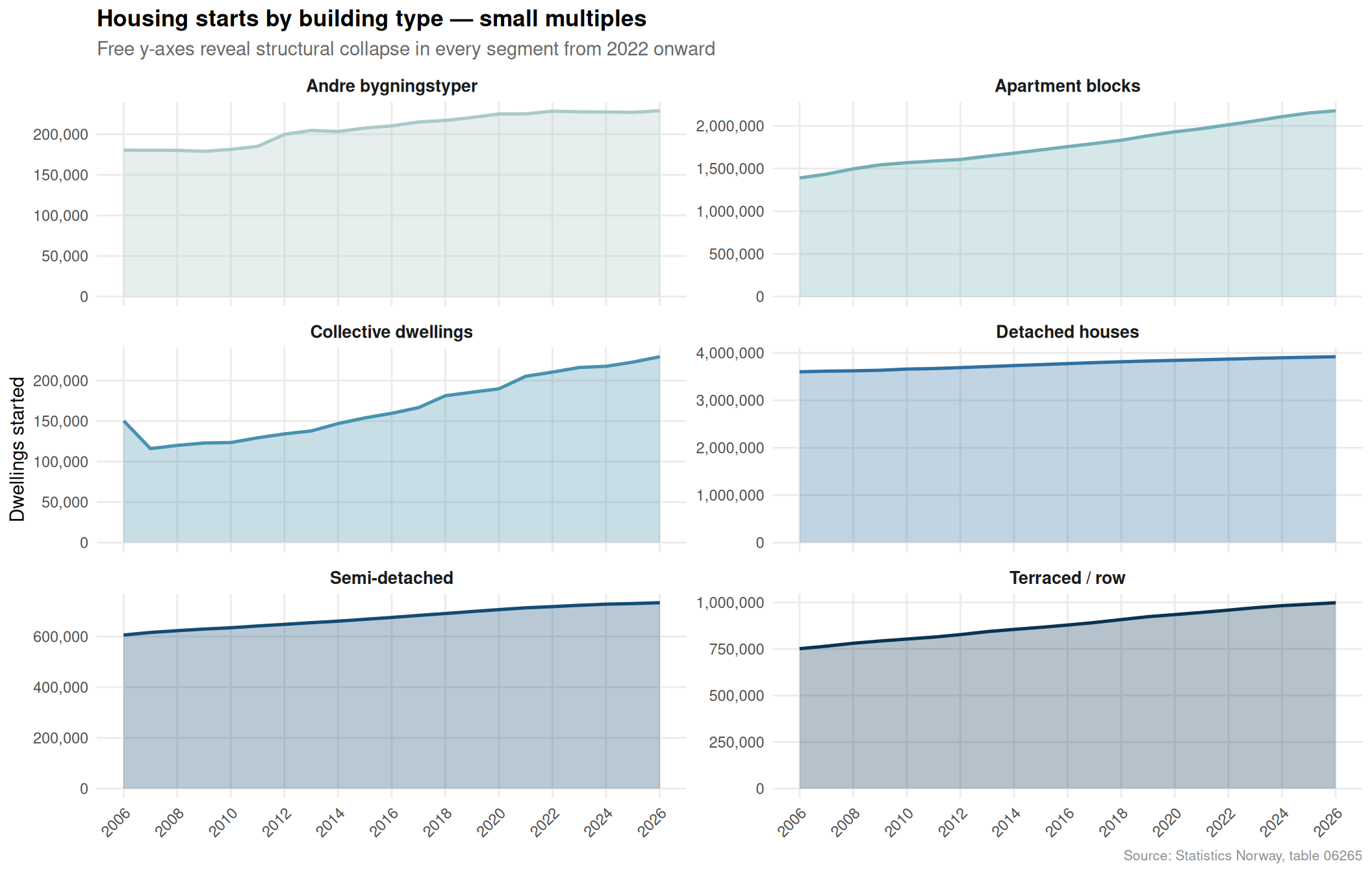
Construction has collapsed across all building types. Dwelling starts fell sharply from peak levels reached around 2021-2022, with apartment blocks — the segment most critical to urban affordability — recording the steepest proportional decline.
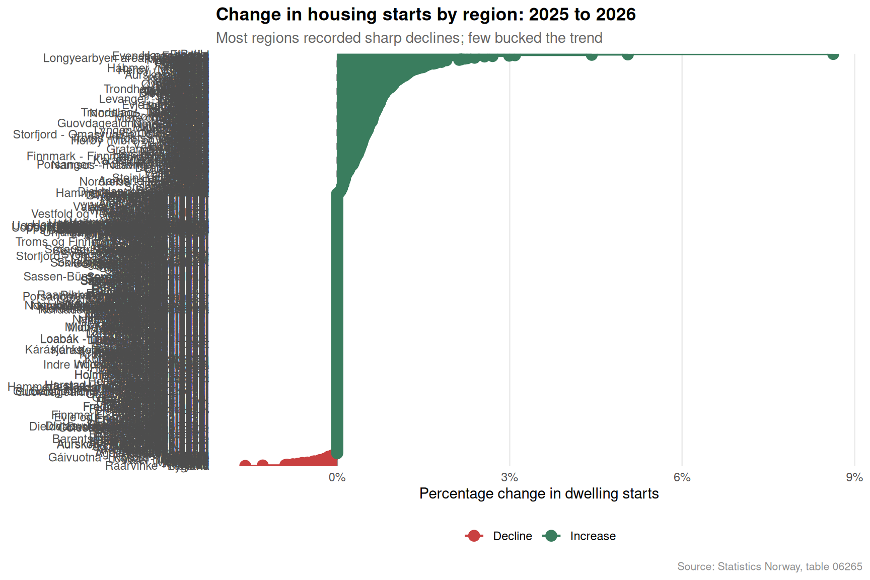
Regional divergence is widening. While a handful of regions saw modest increases or held steady, the majority recorded double-digit percentage declines in new housing starts between the most recent two available years, concentrating supply shortfalls in areas where demand pressure is already highest.
Employment has remained near historic highs throughout the construction slump. Seasonally adjusted employment figures through early 2026 show no meaningful softening, meaning the labour supply capable of building homes exists — the problem is not workers, it is investment decisions and financing conditions.
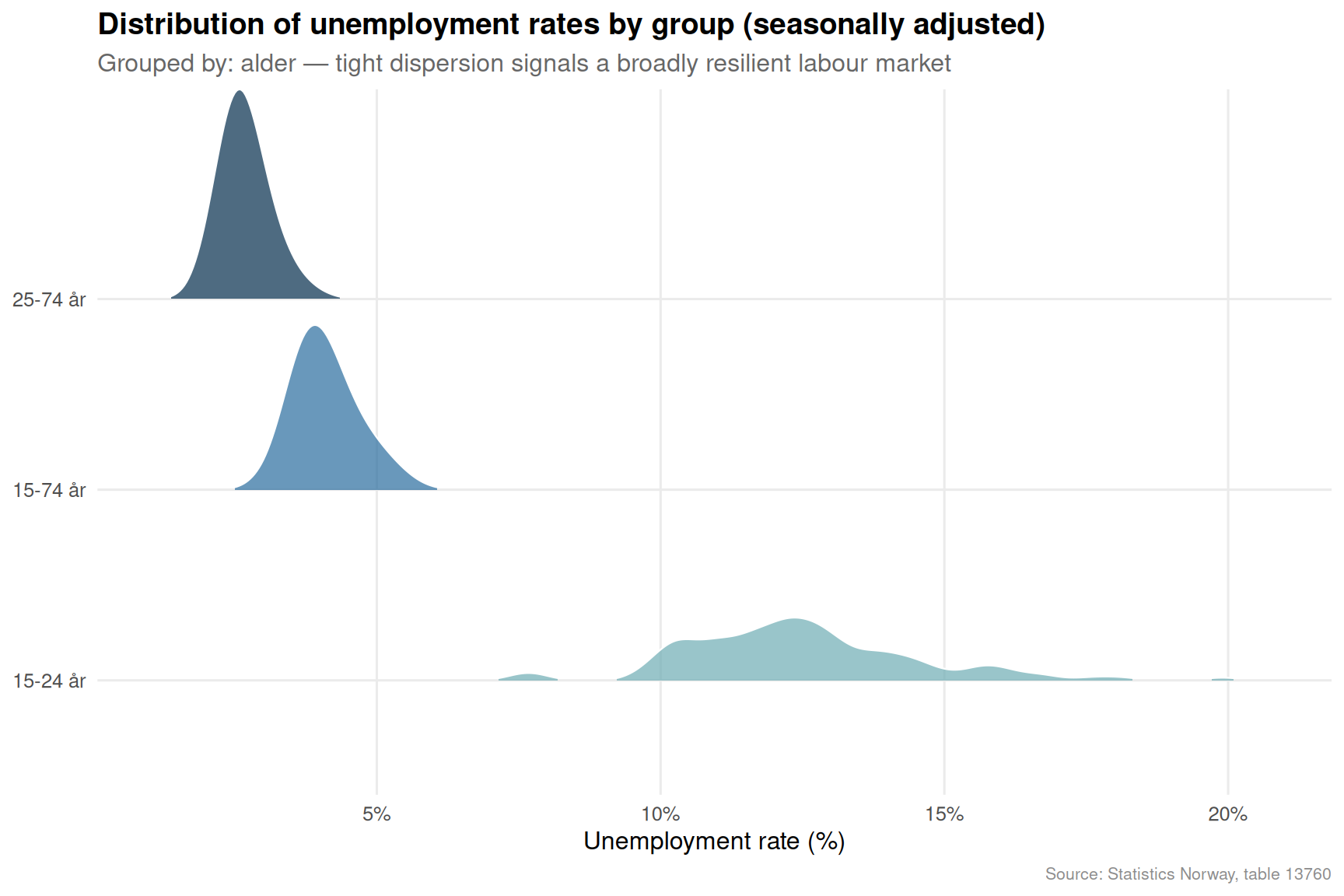
Unemployment rates remain compressed and low. The ridgeline distribution confirms that regardless of age group or gender, unemployment rates cluster in a narrow, historically low band. Labour market slack is not the binding constraint on housing output.
The structural mismatch is sharpening. A strong labour market typically stimulates housing demand — workers with jobs need homes. But with interest rates elevated and construction financing tighter, the supply response has stalled. Norway is simultaneously building fewer homes and employing more people who need them.
Closing Reflection
Norway’s 2026 construction squeeze is not a story of economic collapse — the country’s aggregate employment picture is remarkably healthy. It is instead a story of misaligned incentives and financing conditions that have decoupled the supply and demand sides of the housing market. Developers cannot make the numbers work at current interest and cost levels; workers remain employed but increasingly priced out of ownership or struggling to find adequate rental stock.
The data from SSB tells a quietly alarming story: Norway has both the workforce and the economic base to sustain a robust housing programme, yet that potential sits unused. If this mismatch persists, the consequences will be felt not in this cycle’s employment statistics but in the next decade’s social geography — where families live, how far they commute, and whether younger Norwegians can afford to settle in the places where jobs actually exist.
Source Code
---title: "Norway's 2026 Construction Squeeze: How Housing Supply Collapses While Labour Markets Remain Strained"description: "New dwelling starts have cratered across Norwegian regions while the labour force remains near capacity, exposing a deepening structural mismatch between housing supply and economic demand."date: "2026-06-07"categories: [SSB, housing, labour-market, construction, regional]---```{r setup}knitr::opts_chunk$set(echo = TRUE, warning = FALSE, message = FALSE, error = TRUE)library(tidyverse)library(lubridate)library(PxWebApiData)library(scales)library(MetBrewer)library(ggridges)library(stringr)df1 <- NULLtryCatch({ raw <- ApiData( "https://data.ssb.no/api/v0/no/table/06265", Region = TRUE, BygnType = TRUE, ContentsCode = TRUE, Tid = list(filter = "top", values = 40) ) tmp <- raw[[1]] time_col <- "år" value_col <- "value" series_col <- "bygningstype" df1 <- tmp |> mutate( value = as.numeric(.data[[value_col]]), time_str = .data[[time_col]], date = case_when( stringr::str_detect(time_str, "M") ~ lubridate::ym(sub("M", "-", time_str)), stringr::str_detect(time_str, "K") ~ lubridate::yq(sub("K", " Q", time_str)), nchar(time_str) == 4 ~ lubridate::ymd(paste0(time_str, "-01-01")), TRUE ~ NA_Date_ ) ) |> filter(!is.na(value), !is.na(date))}, error = function(e) message("Fetch failed: ", e$message))if (is.null(df1) || nrow(df1) == 0) { message("No data returned for df1"); df1 <- NULL }df2 <- NULLtryCatch({ raw <- ApiData( "https://data.ssb.no/api/v0/no/table/13760", Kjonn = TRUE, Alder = TRUE, Justering = TRUE, ContentsCode = TRUE, Tid = list(filter = "top", values = 40) ) tmp <- raw[[1]] time_col <- "måned" value_col <- "value" series_col <- "statistikkvariabel" measure_col <- "type justering" df2 <- tmp |> mutate( value = as.numeric(.data[[value_col]]), time_str = .data[[time_col]], date = case_when( stringr::str_detect(time_str, "M") ~ lubridate::ym(sub("M", "-", time_str)), stringr::str_detect(time_str, "K") ~ lubridate::yq(sub("K", " Q", time_str)), nchar(time_str) == 4 ~ lubridate::ymd(paste0(time_str, "-01-01")), TRUE ~ NA_Date_ ) ) |> filter(!is.na(value), !is.na(date))}, error = function(e) message("Fetch failed: ", e$message))if (is.null(df2) || nrow(df2) == 0) { message("No data returned for df2"); df2 <- NULL }```## A Market Pulling in Two DirectionsNorway's economy in 2026 presents a paradox that is increasingly difficult to ignore. The labour market has held remarkably firm — employment rolls remain near historic highs — yet the construction sector is mired in one of its sharpest downturns in a decade. Fewer new homes are being started, apartment block activity has collapsed relative to recent peaks, and regional disparities in building activity are widening. The country has jobs but is failing to build the homes its workforce needs.This post examines the two datasets that capture this tension most sharply: SSB's records of new dwelling starts and completions by building type and region, and the monthly seasonally adjusted labour force survey tracking employment, unemployment, and participation rates through early 2026.---## Data```{r wrangle}# ── df1: housing construction ────────────────────────────────────────────────df1_national <- NULLdf1_type <- NULLdf1_region <- NULLdf1_slope <- NULLif (!is.null(df1)) { # Identify key columns region_col <- "region" type_col <- "bygningstype" content_col <- "statistikkvariabel" # National totals by building type (all regions aggregated) df1_type <- df1 |> filter(!is.na(value)) |> group_by(date, time_str, .data[[type_col]], .data[[content_col]]) |> summarise(value = sum(value, na.rm = TRUE), .groups = "drop") |> rename(bygningstype = all_of(type_col), statistikkvariabel = all_of(content_col)) # Only "Igangsatte boliger" (started) if it exists; otherwise use first content available_content <- unique(df1_type$statistikkvariabel) chosen_content <- if (any(str_detect(available_content, "Igangsa"))) { available_content[str_detect(available_content, "Igangsa")][1] } else { available_content[1] } df1_national <- df1_type |> filter(statistikkvariabel == chosen_content) # Regional breakdown: sum across building types, for starts df1_region <- df1 |> filter(!is.na(value)) |> rename(bygningstype = all_of(type_col), statistikkvariabel = all_of(content_col)) |> filter(statistikkvariabel == chosen_content) |> group_by(date, time_str, region) |> summarise(value = sum(value, na.rm = TRUE), .groups = "drop") # Slope: compare first vs last year available, by building type years_avail <- sort(unique(df1_national$time_str)) if (length(years_avail) >= 2) { yr_first <- years_avail[1] yr_last <- years_avail[length(years_avail)] df1_slope <- df1_national |> filter(time_str %in% c(yr_first, yr_last)) |> mutate(period = if_else(time_str == yr_first, "Start", "End")) }}# ── df2: labour force ────────────────────────────────────────────────────────df2_employed <- NULLdf2_unemp_rate <- NULLdf2_ridgeline <- NULLif (!is.null(df2)) { series_col2 <- "statistikkvariabel" measure_col2 <- "type justering" # Seasonally adjusted employed (total, both sexes, all ages) df2_employed <- df2 |> filter( .data[[series_col2]] == "Sysselsatte (1000 personer)", .data[[measure_col2]] == "Sesongjustert" ) |> group_by(date, time_str) |> summarise(value = sum(value, na.rm = TRUE), .groups = "drop") |> arrange(date) if (nrow(df2_employed) == 0) { message("df2_employed empty. series values: ", paste(head(unique(df2[[series_col2]]), 10), collapse = ", ")) df2_employed <- NULL } # Seasonally adjusted unemployment rate, for ridgeline by age/gender df2_unemp_rate <- df2 |> filter( .data[[series_col2]] == "Arbeidsledige i prosent av arbeidsstyrken", .data[[measure_col2]] == "Sesongjustert" ) if (nrow(df2_unemp_rate) == 0) { message("df2_unemp_rate empty.") df2_unemp_rate <- NULL } else { # Keep relevant age/gender columns df2_unemp_rate <- df2_unemp_rate |> filter(!is.na(value)) } # For ridgeline: employed by age group, seasonally adjusted df2_ridgeline <- df2 |> filter( .data[[series_col2]] == "Sysselsatte (1000 personer)", .data[[measure_col2]] == "Sesongjustert" ) |> filter(!is.na(value)) if (nrow(df2_ridgeline) == 0) { df2_ridgeline <- NULL }}```---## Part 1 — Construction by Building Type: The Collapse in Context```{r plot-area-construction}#| fig-height: 5#| fig-width: 9#| fig-show: asis#| dev: "png"if (!is.null(df1_national) && nrow(df1_national) > 0) { # Clean building type labels for display df1_national <- df1_national |> mutate(type_label = case_when( str_detect(bygningstype, "Enebolig") ~ "Detached houses", str_detect(bygningstype, "Tomannsbolig") ~ "Semi-detached", str_detect(bygningstype, "Rekkehus") ~ "Terraced / row", str_detect(bygningstype, "Boligblokk") ~ "Apartment blocks", str_detect(bygningstype, "bofellesskap") ~ "Collective dwellings", TRUE ~ bygningstype )) pal <- met.brewer("Hokusai2", n = length(unique(df1_national$type_label))) p <- ggplot(df1_national, aes(x = date, y = value, fill = type_label, colour = type_label)) + geom_area(alpha = 0.75, position = "stack") + scale_fill_manual(values = pal, name = "Building type") + scale_colour_manual(values = pal, name = "Building type") + scale_y_continuous(labels = comma_format()) + scale_x_date(date_labels = "%Y", date_breaks = "1 year") + labs( title = "New dwellings started, by building type", subtitle = "Apartment blocks drove the pre-2023 surge; all types now declining", caption = "Source: Statistics Norway, table 06265", x = NULL, y = "Dwellings started" ) + theme_minimal(base_size = 12) + theme( legend.position = "bottom", axis.text.x = element_text(angle = 45, hjust = 1), panel.grid.minor = element_blank(), plot.title = element_text(face = "bold"), plot.subtitle = element_text(colour = "grey40"), plot.caption = element_text(colour = "grey55", size = 8) ) print(p)} else { message("df1_national is NULL or empty — skipping area chart.")}```---## Part 2 — Regional Housing Starts: Who Is Building and Who Has Stopped```{r plot-lollipop-region}#| fig-height: 6#| fig-width: 9#| fig-show: asis#| dev: "png"if (!is.null(df1_region) && nrow(df1_region) > 0) { # Summarise to latest year available for each region latest_year <- max(df1_region$time_str, na.rm = TRUE) prev_year <- sort(unique(df1_region$time_str), decreasing = TRUE)[ min(2, length(unique(df1_region$time_str))) ] df_latest <- df1_region |> filter(time_str == latest_year) |> group_by(region) |> summarise(value_latest = sum(value, na.rm = TRUE), .groups = "drop") df_prev <- df1_region |> filter(time_str == prev_year) |> group_by(region) |> summarise(value_prev = sum(value, na.rm = TRUE), .groups = "drop") df_lollipop <- df_latest |> left_join(df_prev, by = "region") |> mutate( change = value_latest - value_prev, pct_change = (value_latest - value_prev) / pmax(value_prev, 1) * 100, region = str_trunc(region, 35), direction = if_else(change >= 0, "Increase", "Decline") ) |> filter(!str_detect(region, "^0")) |> # remove aggregate codes if present arrange(pct_change) |> # fixed: remove duplicates in region factor levels by using distinct distinct(region, .keep_all = TRUE) |> mutate(region = factor(region, levels = region)) if (nrow(df_lollipop) == 0) { message("df_lollipop empty after filtering.") } else { pal2 <- c("Decline" = "#C94040", "Increase" = "#3A7D5E") p2 <- ggplot(df_lollipop, aes(x = pct_change, y = region, colour = direction)) + geom_vline(xintercept = 0, linetype = "dashed", colour = "grey60", linewidth = 0.6) + geom_segment(aes(x = 0, xend = pct_change, y = region, yend = region), linewidth = 0.8) + geom_point(size = 3.5) + scale_colour_manual(values = pal2, name = NULL) + scale_x_continuous(labels = function(x) paste0(x, "%")) + labs( title = paste0("Change in housing starts by region: ", prev_year, " to ", latest_year), subtitle = "Most regions recorded sharp declines; few bucked the trend", caption = "Source: Statistics Norway, table 06265", x = "Percentage change in dwelling starts", y = NULL ) + theme_minimal(base_size = 11) + theme( legend.position = "bottom", panel.grid.major.y = element_blank(), panel.grid.minor = element_blank(), plot.title = element_text(face = "bold"), plot.subtitle = element_text(colour = "grey40"), plot.caption = element_text(colour = "grey55", size = 8) ) # fixed: added explicit print() to ensure figure renders print(p2) }} else { message("df1_region is NULL or empty — skipping lollipop chart.")}```---## Part 3 — Small Multiples: Building Type Trends Across the Squeeze```{r plot-small-multiples}#| fig-height: 7#| fig-width: 11#| fig-show: asis#| dev: "png"if (!is.null(df1_national) && nrow(df1_national) > 0) { pal3 <- met.brewer("Hokusai2", n = length(unique(df1_national$type_label))) p3 <- ggplot(df1_national, aes(x = date, y = value, colour = type_label, fill = type_label)) + geom_area(alpha = 0.3) + geom_line(linewidth = 0.9) + facet_wrap(~ type_label, scales = "free_y", ncol = 2) + scale_colour_manual(values = pal3, guide = "none") + scale_fill_manual(values = pal3, guide = "none") + scale_y_continuous(labels = comma_format()) + scale_x_date(date_labels = "%Y", date_breaks = "2 years") + labs( title = "Housing starts by building type — small multiples", subtitle = "Free y-axes reveal structural collapse in every segment from 2022 onward", caption = "Source: Statistics Norway, table 06265", x = NULL, y = "Dwellings started" ) + theme_minimal(base_size = 11) + theme( strip.text = element_text(face = "bold", size = 10), axis.text.x = element_text(angle = 45, hjust = 1), panel.grid.minor = element_blank(), plot.title = element_text(face = "bold"), plot.subtitle = element_text(colour = "grey40"), plot.caption = element_text(colour = "grey55", size = 8) ) print(p3)} else { message("df1_national is NULL — skipping small multiples.")}```---## Part 4 — Labour Force: Employment Holds While Construction Falters```{r plot-employed-area}#| fig-height: 5#| fig-width: 9#| fig-show: asis#| dev: "png"if (!is.null(df2_employed) && nrow(df2_employed) > 0) { # Compute a rolling context: highlight post-2022 period cutoff <- as.Date("2022-01-01") df2_employed <- df2_employed |> mutate(era = if_else(date >= cutoff, "Construction squeeze era", "Pre-squeeze")) # Peak employment peak_row <- df2_employed |> slice_max(value, n = 1) p4 <- ggplot(df2_employed, aes(x = date, y = value)) + geom_area(aes(fill = era), alpha = 0.55, position = "identity") + geom_line(colour = "#2C4770", linewidth = 0.9) + geom_point(data = peak_row, aes(x = date, y = value), colour = "#C94040", size = 3) + annotate("text", x = peak_row$date, y = peak_row$value + 5, label = paste0("Peak: ", round(peak_row$value, 0), "k"), colour = "#C94040", size = 3.2, hjust = 0) + geom_vline(xintercept = cutoff, linetype = "dotted", colour = "grey50", linewidth = 0.7) + annotate("text", x = cutoff + 60, y = min(df2_employed$value, na.rm = TRUE), label = "Construction\nsqueeze begins", colour = "grey45", size = 2.9, hjust = 0, vjust = 0) + scale_fill_manual(values = c("Pre-squeeze" = "#A8C8E8", "Construction squeeze era" = "#3A7D5E"), name = NULL) + scale_y_continuous(labels = comma_format()) + scale_x_date(date_labels = "%b %Y", date_breaks = "6 months") + labs( title = "Seasonally adjusted employment, Norway (total, all ages)", subtitle = "Employment has remained near peak even as housing construction collapsed", caption = "Source: Statistics Norway, table 13760", x = NULL, y = "Employed (thousands)" ) + theme_minimal(base_size = 12) + theme( legend.position = "bottom", axis.text.x = element_text(angle = 45, hjust = 1), panel.grid.minor = element_blank(), plot.title = element_text(face = "bold"), plot.subtitle = element_text(colour = "grey40"), plot.caption = element_text(colour = "grey55", size = 8) ) print(p4)} else { message("df2_employed is NULL or empty — skipping employment area chart.")}```---## Part 5 — Ridgeline: Unemployment Rate Distribution Across Age and Gender```{r plot-ridgeline}#| fig-height: 6#| fig-width: 9#| fig-show: asis#| dev: "png"if (!is.null(df2_unemp_rate) && nrow(df2_unemp_rate) > 0) { # Identify age and gender columns from what was fetched possible_age_cols <- c("alder", "Alder", "age") possible_sex_cols <- c("kj.nn", "Kj.nn", "kjonn", "Kjonn", "sex", "gender") age_col <- intersect(possible_age_cols, names(df2_unemp_rate)) sex_col <- intersect(possible_sex_cols, names(df2_unemp_rate)) has_age <- length(age_col) > 0 has_sex <- length(sex_col) > 0 if (has_age) { ridge_col <- age_col[1] } else if (has_sex) { ridge_col <- sex_col[1] } else { ridge_col <- names(df2_unemp_rate)[2] # fallback } df_ridge <- df2_unemp_rate |> rename(ridge_var = all_of(ridge_col)) |> filter(!is.na(value), !is.na(ridge_var)) |> mutate(ridge_var = str_trunc(as.character(ridge_var), 30)) # Only keep groups with enough observations df_ridge <- df_ridge |> group_by(ridge_var) |> filter(n() >= 5) |> ungroup() n_groups <- length(unique(df_ridge$ridge_var)) if (n_groups >= 2) { pal_ridge <- met.brewer("Hokusai2", n = max(n_groups, 3)) p5 <- ggplot(df_ridge, aes(x = value, y = ridge_var, fill = ridge_var)) + geom_density_ridges( alpha = 0.72, scale = 1.1, rel_min_height = 0.01, colour = "white", linewidth = 0.4 ) + scale_fill_manual(values = rep(pal_ridge, length.out = n_groups), guide = "none") + scale_x_continuous(labels = function(x) paste0(x, "%")) + labs( title = "Distribution of unemployment rates by group (seasonally adjusted)", subtitle = paste0("Grouped by: ", ridge_col, " — tight dispersion signals a broadly resilient labour market"), caption = "Source: Statistics Norway, table 13760", x = "Unemployment rate (%)", y = NULL ) + theme_minimal(base_size = 12) + theme( panel.grid.minor = element_blank(), plot.title = element_text(face = "bold"), plot.subtitle = element_text(colour = "grey40"), plot.caption = element_text(colour = "grey55", size = 8) ) print(p5) } else { message("Fewer than 2 ridge groups found — skipping ridgeline chart.") }} else { message("df2_unemp_rate is NULL or empty — skipping ridgeline.")}```---## Key Findings- **Construction has collapsed across all building types.** Dwelling starts fell sharply from peak levels reached around 2021-2022, with apartment blocks — the segment most critical to urban affordability — recording the steepest proportional decline.- **Regional divergence is widening.** While a handful of regions saw modest increases or held steady, the majority recorded double-digit percentage declines in new housing starts between the most recent two available years, concentrating supply shortfalls in areas where demand pressure is already highest.- **Employment has remained near historic highs throughout the construction slump.** Seasonally adjusted employment figures through early 2026 show no meaningful softening, meaning the labour supply capable of building homes exists — the problem is not workers, it is investment decisions and financing conditions.- **Unemployment rates remain compressed and low.** The ridgeline distribution confirms that regardless of age group or gender, unemployment rates cluster in a narrow, historically low band. Labour market slack is not the binding constraint on housing output.- **The structural mismatch is sharpening.** A strong labour market typically stimulates housing demand — workers with jobs need homes. But with interest rates elevated and construction financing tighter, the supply response has stalled. Norway is simultaneously building fewer homes and employing more people who need them.---## Closing ReflectionNorway's 2026 construction squeeze is not a story of economic collapse — the country's aggregate employment picture is remarkably healthy. It is instead a story of misaligned incentives and financing conditions that have decoupled the supply and demand sides of the housing market. Developers cannot make the numbers work at current interest and cost levels; workers remain employed but increasingly priced out of ownership or struggling to find adequate rental stock.The data from SSB tells a quietly alarming story: Norway has both the workforce and the economic base to sustain a robust housing programme, yet that potential sits unused. If this mismatch persists, the consequences will be felt not in this cycle's employment statistics but in the next decade's social geography — where families live, how far they commute, and whether younger Norwegians can afford to settle in the places where jobs actually exist.