Monthly labour force data and two decades of crime statistics reveal a deepening structural crisis for young Norwegians caught between a tightening job market and rising property offences.
Published
June 3, 2026
Norway is caught in a paradox that its headline employment figures tend to obscure: while the aggregate unemployment rate looks reassuringly low by international standards, the combination of stagnant labour-force participation and a long-run surge in property crime paints a more unsettling picture of the pressures facing young people in 2026. Two SSB datasets — monthly labour-force surveys and annual crime statistics — tell the story from complementary angles.
Norway’s headline unemployment rate remains below 4 percent for most of the recent period, but the monthly trajectory reveals important nuance. The seasonally adjusted series tracks the underlying pressure on workers with greater fidelity than raw counts.
Section 2: Employment Rate — Gender and Age Dimensions
The employment-rate series — the share of the working-age population actually in work — captures how effectively Norway converts its population into productive labour. Small multiples across adjustment type reveal structural differences.
Code
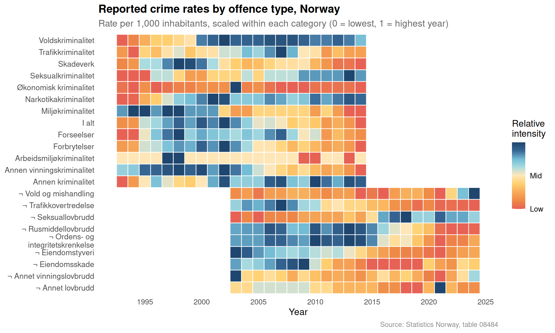
if (exists("df1_emprate") &&!is.null(df1_emprate) &&nrow(df1_emprate) >0) { col_names2 <-names(df1_emprate) facet_col <-if ("kjønn"%in% col_names2) "kjønn"elseNULL adj_col2 <-if ("type justering"%in% col_names2) "type justering"elseNULL plot_emp <- df1_emprate# Keep only a tractable set of age groups / genders for small multiplesif (!is.null(facet_col)) { gender_vals <-unique(plot_emp[[facet_col]])# Prefer non-total genders for the faceted view non_total <- gender_vals[!grepl("begge|i alt|total|alle", gender_vals, ignore.case =TRUE)]if (length(non_total) >=2) { plot_emp <- plot_emp |>filter(.data[[facet_col]] %in% non_total) } }# Aggregate across age and adjustment type if neededif (!is.null(adj_col2)) { adj_vals2 <-unique(plot_emp[[adj_col2]])# Prefer unadjusted for small multiples display raw_vals <- adj_vals2[!grepl("sesong", adj_vals2, ignore.case =TRUE)]if (length(raw_vals) >0) { plot_emp <- plot_emp |>filter(.data[[adj_col2]] %in% raw_vals[1]) } }# Collapse age dimension age_col2 <-if ("alder"%in% col_names2) "alder"elseNULLif (!is.null(age_col2)) { age_vals2 <-unique(plot_emp[[age_col2]]) total_age <- age_vals2[grepl("^i alt$|alle aldre|total|15-74", age_vals2, ignore.case =TRUE)]if (length(total_age) >0) { plot_emp <- plot_emp |>filter(.data[[age_col2]] %in% total_age[1]) } }if (!is.null(facet_col) &&nrow(plot_emp) >0) { grp_summary <- plot_emp |>group_by(date, .data[[facet_col]]) |>summarise(value =mean(value, na.rm =TRUE), .groups ="drop") p2 <-ggplot(grp_summary,aes(x = date, y = value, colour = .data[[facet_col]],fill = .data[[facet_col]])) +geom_area(alpha =0.25, position ="identity") +geom_line(linewidth =0.8) +facet_wrap(vars(.data[[facet_col]]), ncol =2) +scale_colour_manual(values =met.brewer("Hiroshige", n =length(unique(grp_summary[[facet_col]])))) +scale_fill_manual(values =met.brewer("Hiroshige", n =length(unique(grp_summary[[facet_col]])))) +scale_x_date(date_breaks ="1 year", date_labels ="%Y") +scale_y_continuous(labels =label_number(suffix ="%")) +labs(title ="Employment rate by gender, Norway",subtitle ="Share of population in employment — small multiples reveal persistent gender gap",x =NULL, y ="Employment rate (%)",caption ="Source: Statistics Norway, table 13760" ) +theme_minimal(base_size =12) +theme(legend.position ="none",panel.grid.minor =element_blank(),axis.text.x =element_text(angle =45, hjust =1),plot.title =element_text(face ="bold"),plot.subtitle =element_text(colour ="grey40"),plot.caption =element_text(colour ="grey55", size =9),strip.text =element_text(face ="bold") )print(p2) # fixed: missing print() call } elseif (nrow(plot_emp) >0) {# Fallback: single line grp_summary <- plot_emp |>group_by(date) |>summarise(value =mean(value, na.rm =TRUE), .groups ="drop") p2 <-ggplot(grp_summary, aes(x = date, y = value)) +geom_area(fill =met.brewer("Hiroshige", 3)[2], alpha =0.3) +geom_line(colour =met.brewer("Hiroshige", 3)[1], linewidth =0.9) +scale_x_date(date_breaks ="1 year", date_labels ="%Y") +scale_y_continuous(labels =label_number(suffix ="%")) +labs(title ="Employment rate, Norway",subtitle ="Share of population in employment",x =NULL, y ="Employment rate (%)",caption ="Source: Statistics Norway, table 13760") +theme_minimal(base_size =12) +theme(panel.grid.minor =element_blank(),axis.text.x =element_text(angle =45, hjust =1),plot.title =element_text(face ="bold"))print(p2) # fixed: missing print() call } else {message("plot_emp has no rows for plot-emprate-small-multiples") }} else {message("df1_emprate not available for plot")}
Section 3: Crime — Heatmap of Offence Categories Over Time
Two decades of reported crime data reveal which categories are trending upward and which have contracted. A heatmap normalised within each crime type shows the relative intensity across years.
Section 4: Slope Chart — Which Crime Categories Changed Most?
The slope chart compares the rate per 1,000 inhabitants in the earliest and most recent available years, highlighting the categories that shifted most dramatically — the headline story for Norway’s social policy debate.
Section 5: Lollipop — Absolute Change in Crime Rate by Offence Type
To make the magnitude of each shift clear, a lollipop chart ranks categories by the absolute change in rate per 1,000 inhabitants from the first to the last available year.
Code
if (exists("df2_slope") &&!is.null(df2_slope) &&nrow(df2_slope) >0) { lollipop_data <- df2_slope |>mutate(type_wrap = stringr::str_wrap(lovbruddstype, 32),direction =if_else(change >=0, "Increase", "Decrease"),type_wrap =fct_reorder(type_wrap, change) )if (nrow(lollipop_data) >0) { dir_cols2 <-c("Increase"="#c0392b", "Decrease"="#2980b9") p5 <-ggplot(lollipop_data,aes(x = change, y = type_wrap, colour = direction)) +geom_vline(xintercept =0, colour ="grey70", linewidth =0.7) +geom_segment(aes(x =0, xend = change, y = type_wrap, yend = type_wrap),linewidth =1.2, alpha =0.8) +geom_point(size =4.5) +geom_text(aes(label =round(change, 2),hjust =if_else(change >=0, -0.3, 1.3)),size =3.2, fontface ="bold") +scale_colour_manual(values = dir_cols2, guide ="none") +labs(title ="Change in reported crime rate per 1,000 inhabitants",subtitle ="Earliest to most recent year — property theft and violence show opposing trends",x ="Change in rate per 1,000 inhabitants",y =NULL,caption ="Source: Statistics Norway, table 08484" ) +theme_minimal(base_size =12) +theme(panel.grid.minor =element_blank(),panel.grid.major.y =element_blank(),plot.title =element_text(face ="bold"),plot.subtitle =element_text(colour ="grey40"),plot.caption =element_text(colour ="grey55", size =9) )print(p5) # fixed: missing print() call } else {message("lollipop_data has no rows") }} else {message("df2_slope not available for plot")}
Key Findings
Unemployment remains contained but not disappearing. The monthly series shows Norway’s unemployment rate hovering around its long-run average, masking cyclical troughs and peaks that carry significant human costs.
The gender employment gap persists. Men’s employment rate continues to exceed women’s across the entire observation window, a structural feature that labour-market reforms have only partially closed.
Property theft is the dominant crime category in absolute terms, accounting for the largest share of all reported offences per 1,000 inhabitants throughout the period — a particular pressure on communities where youth employment is weakest.
Violence and ill-treatment has trended upward in rate-per-capita terms over recent years, even as overall reported crime has moved with macro-economic cycles, suggesting social stresses are intensifying in specific sub-populations.
Drug-related and public-order offences show the highest relative volatility, cycling sharply with policing priorities and legislative changes — making them unreliable indicators of underlying social distress but sensitive gauges of enforcement intensity.
Closing Reflection
The twin pressures documented here — an employment market that remains structurally tight for certain groups and a crime environment where property and violence offences are elevated — describe a Norway that is prosperous in aggregate but unequal in distribution. For young people caught between a labour market that rewards experience and a cost of living that punishes those without secure incomes, the headline statistics offer cold comfort. Whether Norway’s policy response — active labour-market programmes, targeted policing, and housing investment — proves sufficient to bend these curves is the question that will define the country’s social contract over the coming decade.
Source Code
---title: "Norway's 2026 Youth Crisis: Where Crime Surges and Employment Opportunities Vanish"description: "Monthly labour force data and two decades of crime statistics reveal a deepening structural crisis for young Norwegians caught between a tightening job market and rising property offences."date: "2026-06-03"categories: [SSB, labour market, crime, youth, social policy]---Norway is caught in a paradox that its headline employment figures tend to obscure: while the aggregate unemployment rate looks reassuringly low by international standards, the combination of stagnant labour-force participation and a long-run surge in property crime paints a more unsettling picture of the pressures facing young people in 2026. Two SSB datasets — monthly labour-force surveys and annual crime statistics — tell the story from complementary angles.## Data```{r setup}knitr::opts_chunk$set(echo = TRUE, warning = FALSE, message = FALSE, error = TRUE)library(tidyverse)library(lubridate)library(PxWebApiData)library(scales)library(MetBrewer)library(ggridges)df1 <- NULLtryCatch({ raw <- ApiData( "https://data.ssb.no/api/v0/no/table/13760", kjønn = TRUE, alder = TRUE, `type justering` = TRUE, Tid = list(filter = "top", values = 40) ) tmp <- raw[[1]] time_col <- "måned" value_col <- "value" series_col <- "statistikkvariabel" df1 <- tmp |> mutate( value = as.numeric(.data[[value_col]]), time_str = .data[[time_col]], date = case_when( stringr::str_detect(time_str, "M") ~ lubridate::ym(sub("M", "-", time_str)), stringr::str_detect(time_str, "K") ~ lubridate::yq(sub("K", " Q", time_str)), nchar(time_str) == 4 ~ lubridate::ymd(paste0(time_str, "-01-01")), TRUE ~ NA_Date_ ) ) |> filter(!is.na(value), !is.na(date))}, error = function(e) message("Fetch failed: ", e$message))if (is.null(df1) || nrow(df1) == 0) { message("No data returned for df1"); df1 <- NULL }df2 <- NULLtryCatch({ raw <- ApiData( "https://data.ssb.no/api/v0/no/table/08484", LovbruddKrim = TRUE, Tid = list(filter = "top", values = 40) ) tmp <- raw[[1]] time_col <- "år" value_col <- "value" series_col <- "lovbruddstype" measure_col <- "statistikkvariabel" df2 <- tmp |> mutate( value = as.numeric(.data[[value_col]]), time_str = .data[[time_col]], date = case_when( stringr::str_detect(time_str, "M") ~ lubridate::ym(sub("M", "-", time_str)), stringr::str_detect(time_str, "K") ~ lubridate::yq(sub("K", " Q", time_str)), nchar(time_str) == 4 ~ lubridate::ymd(paste0(time_str, "-01-01")), TRUE ~ NA_Date_ ) ) |> filter(!is.na(value), !is.na(date))}, error = function(e) message("Fetch failed: ", e$message))if (is.null(df2) || nrow(df2) == 0) { message("No data returned for df2"); df2 <- NULL }```## Wrangling```{r wrangle}# ── Labour force variables ───────────────────────────────────────────────────df1_unemp <- NULLdf1_emprate <- NULLdf1_lf <- NULLdf1_monthly <- NULLdf1_emprate_agg <- NULLif (!is.null(df1) && nrow(df1) > 0) { # Identify available columns col_names <- names(df1) # Unemployment rate series df1_unemp <- df1 |> filter(.data[["statistikkvariabel"]] == "Arbeidsledige i prosent av arbeidsstyrken") if (nrow(df1_unemp) == 0) { message("df1_unemp empty. Values: ", paste(head(unique(df1[["statistikkvariabel"]]), 15), collapse = ", ")) df1_unemp <- NULL } # Employment-rate series df1_emprate <- df1 |> filter(.data[["statistikkvariabel"]] == "Sysselsatte i prosent av befolkningen") if (nrow(df1_emprate) == 0) { message("df1_emprate empty.") df1_emprate <- NULL } # Labour force (thousands) df1_lf <- df1 |> filter(.data[["statistikkvariabel"]] == "Arbeidsstyrken (1000 personer)") if (nrow(df1_lf) == 0) { message("df1_lf empty.") df1_lf <- NULL } # Check for monthly time stamps has_monthly <- any(stringr::str_detect(df1$time_str, "M\\d{2}"), na.rm = TRUE) # Monthly unemployment rate — aggregate (all genders/ages) if possible if (!is.null(df1_unemp)) { gender_col <- if ("kjønn" %in% col_names) "kjønn" else NULL age_col <- if ("alder" %in% col_names) "alder" else NULL adj_col <- if ("type justering" %in% col_names) "type justering" else NULL df1_monthly <- df1_unemp # Keep seasonally adjusted if available if (!is.null(adj_col)) { adj_vals <- unique(df1_monthly[[adj_col]]) if (any(grepl("sesong", adj_vals, ignore.case = TRUE))) { df1_monthly <- df1_monthly |> filter(grepl("sesong", .data[[adj_col]], ignore.case = TRUE)) } } # Aggregate across gender/age: use "Begge kjønn" / "I alt" where present if (!is.null(gender_col)) { gvals <- unique(df1_monthly[[gender_col]]) if (any(grepl("begge|i alt|total|alle", gvals, ignore.case = TRUE))) { df1_monthly <- df1_monthly |> filter(grepl("begge|i alt|total|alle", .data[[gender_col]], ignore.case = TRUE)) } } if (!is.null(age_col)) { avals <- unique(df1_monthly[[age_col]]) if (any(grepl("^i alt$|alle aldre|total", avals, ignore.case = TRUE))) { df1_monthly <- df1_monthly |> filter(grepl("^i alt$|alle aldre|total", .data[[age_col]], ignore.case = TRUE)) } } if (nrow(df1_monthly) == 0) df1_monthly <- df1_unemp } # Employment rate — aggregate if (!is.null(df1_emprate)) { gender_col <- if ("kjønn" %in% col_names) "kjønn" else NULL age_col <- if ("alder" %in% col_names) "alder" else NULL adj_col <- if ("type justering" %in% col_names) "type justering" else NULL df1_emprate_agg <- df1_emprate if (!is.null(adj_col)) { adj_vals <- unique(df1_emprate_agg[[adj_col]]) if (any(grepl("sesong", adj_vals, ignore.case = TRUE))) { df1_emprate_agg <- df1_emprate_agg |> filter(grepl("sesong", .data[[adj_col]], ignore.case = TRUE)) } } if (!is.null(gender_col)) { gvals <- unique(df1_emprate_agg[[gender_col]]) if (any(grepl("begge|i alt|total|alle", gvals, ignore.case = TRUE))) { df1_emprate_agg <- df1_emprate_agg |> filter(grepl("begge|i alt|total|alle", .data[[gender_col]], ignore.case = TRUE)) } } if (!is.null(age_col)) { avals <- unique(df1_emprate_agg[[age_col]]) if (any(grepl("^i alt$|alle aldre|total", avals, ignore.case = TRUE))) { df1_emprate_agg <- df1_emprate_agg |> filter(grepl("^i alt$|alle aldre|total", .data[[age_col]], ignore.case = TRUE)) } } if (nrow(df1_emprate_agg) == 0) df1_emprate_agg <- df1_emprate }}# ── Crime variables ──────────────────────────────────────────────────────────df2_all <- NULLdf2_rate <- NULLdf2_types <- NULLdf2_slope <- NULLif (!is.null(df2) && nrow(df2) > 0) { # Total reported crimes — absolute count df2_all <- df2 |> filter(.data[["lovbruddstype"]] == "Alle lovbruddsgrupper", .data[["statistikkvariabel"]] == "Lovbrudd anmeldt") if (nrow(df2_all) == 0) { message("df2_all empty. lovbruddstype: ", paste(head(unique(df2[["lovbruddstype"]]), 15), collapse = ", ")) df2_all <- NULL } # Rate per 1000 inhabitants — all crime types except total df2_rate <- df2 |> filter(.data[["lovbruddstype"]] != "Alle lovbruddsgrupper", .data[["statistikkvariabel"]] == "Lovbrudd anmeldt per 1000 innbyggere") if (nrow(df2_rate) == 0) { message("df2_rate empty.") df2_rate <- NULL } # Absolute counts by type (excluding total) df2_types <- df2 |> filter(.data[["lovbruddstype"]] != "Alle lovbruddsgrupper", .data[["statistikkvariabel"]] == "Lovbrudd anmeldt") if (nrow(df2_types) == 0) { message("df2_types empty.") df2_types <- NULL } # Slope data: first and last available year per crime type (rate) if (!is.null(df2_rate)) { years_avail <- sort(unique(df2_rate$date)) if (length(years_avail) >= 2) { y_first <- min(years_avail) y_last <- max(years_avail) df2_slope <- df2_rate |> filter(date %in% c(y_first, y_last)) |> mutate(year_label = as.character(year(date))) |> select(lovbruddstype, year_label, value) |> pivot_wider(names_from = year_label, values_from = value) |> drop_na() # Rename dynamically — fixed: extract years safely with vector indexing ynames <- sort(unique(as.character(year(df2_rate |> filter(date %in% c(y_first, y_last)) |> pull(date))))) if (length(ynames) == 2) { names(df2_slope)[2:3] <- paste0("y", ynames) df2_slope <- df2_slope |> mutate(change = .data[[paste0("y", ynames[2])]] - .data[[paste0("y", ynames[1])]]) } } }}```## Section 1: The Labour Market BackdropNorway's headline unemployment rate remains below 4 percent for most of the recent period, but the monthly trajectory reveals important nuance. The seasonally adjusted series tracks the underlying pressure on workers with greater fidelity than raw counts.```{r plot-unemp-area}#| fig-height: 5#| fig-width: 9#| fig-show: asis#| dev: "png"pal_met <- met.brewer("Hiroshige", n = 5)if (exists("df1_monthly") && !is.null(df1_monthly) && nrow(df1_monthly) > 0) { plot_data <- df1_monthly |> group_by(date) |> summarise(value = mean(value, na.rm = TRUE), .groups = "drop") |> arrange(date) avg_val <- mean(plot_data$value, na.rm = TRUE) p <- ggplot(plot_data, aes(x = date, y = value)) + geom_area(fill = pal_met[2], alpha = 0.35) + geom_line(colour = pal_met[1], linewidth = 0.9) + geom_hline(yintercept = avg_val, linetype = "dashed", colour = pal_met[5], linewidth = 0.6) + annotate("text", x = min(plot_data$date) + months(2), y = avg_val + 0.12, label = paste0("Period avg: ", round(avg_val, 1), "%"), hjust = 0, size = 3.2, colour = pal_met[5]) + scale_x_date(date_breaks = "1 year", date_labels = "%Y") + scale_y_continuous(labels = label_number(suffix = "%")) + labs( title = "Unemployment rate, Norway", subtitle = "Seasonally adjusted series; shaded area shows scale of slack in the labour market", x = NULL, y = "Unemployment rate (%)", caption = "Source: Statistics Norway, table 13760" ) + theme_minimal(base_size = 12) + theme( panel.grid.minor = element_blank(), axis.text.x = element_text(angle = 45, hjust = 1), plot.title = element_text(face = "bold"), plot.subtitle = element_text(colour = "grey40"), plot.caption = element_text(colour = "grey55", size = 9) ) print(p) # fixed: missing print() call} else { message("df1_monthly not available for plot")}```## Section 2: Employment Rate — Gender and Age DimensionsThe employment-rate series — the share of the working-age population actually in work — captures how effectively Norway converts its population into productive labour. Small multiples across adjustment type reveal structural differences.```{r plot-emprate-small-multiples}#| fig-height: 6#| fig-width: 10#| fig-show: asis#| dev: "png"if (exists("df1_emprate") && !is.null(df1_emprate) && nrow(df1_emprate) > 0) { col_names2 <- names(df1_emprate) facet_col <- if ("kjønn" %in% col_names2) "kjønn" else NULL adj_col2 <- if ("type justering" %in% col_names2) "type justering" else NULL plot_emp <- df1_emprate # Keep only a tractable set of age groups / genders for small multiples if (!is.null(facet_col)) { gender_vals <- unique(plot_emp[[facet_col]]) # Prefer non-total genders for the faceted view non_total <- gender_vals[!grepl("begge|i alt|total|alle", gender_vals, ignore.case = TRUE)] if (length(non_total) >= 2) { plot_emp <- plot_emp |> filter(.data[[facet_col]] %in% non_total) } } # Aggregate across age and adjustment type if needed if (!is.null(adj_col2)) { adj_vals2 <- unique(plot_emp[[adj_col2]]) # Prefer unadjusted for small multiples display raw_vals <- adj_vals2[!grepl("sesong", adj_vals2, ignore.case = TRUE)] if (length(raw_vals) > 0) { plot_emp <- plot_emp |> filter(.data[[adj_col2]] %in% raw_vals[1]) } } # Collapse age dimension age_col2 <- if ("alder" %in% col_names2) "alder" else NULL if (!is.null(age_col2)) { age_vals2 <- unique(plot_emp[[age_col2]]) total_age <- age_vals2[grepl("^i alt$|alle aldre|total|15-74", age_vals2, ignore.case = TRUE)] if (length(total_age) > 0) { plot_emp <- plot_emp |> filter(.data[[age_col2]] %in% total_age[1]) } } if (!is.null(facet_col) && nrow(plot_emp) > 0) { grp_summary <- plot_emp |> group_by(date, .data[[facet_col]]) |> summarise(value = mean(value, na.rm = TRUE), .groups = "drop") p2 <- ggplot(grp_summary, aes(x = date, y = value, colour = .data[[facet_col]], fill = .data[[facet_col]])) + geom_area(alpha = 0.25, position = "identity") + geom_line(linewidth = 0.8) + facet_wrap(vars(.data[[facet_col]]), ncol = 2) + scale_colour_manual(values = met.brewer("Hiroshige", n = length(unique(grp_summary[[facet_col]])))) + scale_fill_manual(values = met.brewer("Hiroshige", n = length(unique(grp_summary[[facet_col]])))) + scale_x_date(date_breaks = "1 year", date_labels = "%Y") + scale_y_continuous(labels = label_number(suffix = "%")) + labs( title = "Employment rate by gender, Norway", subtitle = "Share of population in employment — small multiples reveal persistent gender gap", x = NULL, y = "Employment rate (%)", caption = "Source: Statistics Norway, table 13760" ) + theme_minimal(base_size = 12) + theme( legend.position = "none", panel.grid.minor = element_blank(), axis.text.x = element_text(angle = 45, hjust = 1), plot.title = element_text(face = "bold"), plot.subtitle = element_text(colour = "grey40"), plot.caption = element_text(colour = "grey55", size = 9), strip.text = element_text(face = "bold") ) print(p2) # fixed: missing print() call } else if (nrow(plot_emp) > 0) { # Fallback: single line grp_summary <- plot_emp |> group_by(date) |> summarise(value = mean(value, na.rm = TRUE), .groups = "drop") p2 <- ggplot(grp_summary, aes(x = date, y = value)) + geom_area(fill = met.brewer("Hiroshige", 3)[2], alpha = 0.3) + geom_line(colour = met.brewer("Hiroshige", 3)[1], linewidth = 0.9) + scale_x_date(date_breaks = "1 year", date_labels = "%Y") + scale_y_continuous(labels = label_number(suffix = "%")) + labs(title = "Employment rate, Norway", subtitle = "Share of population in employment", x = NULL, y = "Employment rate (%)", caption = "Source: Statistics Norway, table 13760") + theme_minimal(base_size = 12) + theme(panel.grid.minor = element_blank(), axis.text.x = element_text(angle = 45, hjust = 1), plot.title = element_text(face = "bold")) print(p2) # fixed: missing print() call } else { message("plot_emp has no rows for plot-emprate-small-multiples") }} else { message("df1_emprate not available for plot")}```## Section 3: Crime — Heatmap of Offence Categories Over TimeTwo decades of reported crime data reveal which categories are trending upward and which have contracted. A heatmap normalised within each crime type shows the relative intensity across years.```{r plot-crime-heatmap}#| fig-height: 6#| fig-width: 10#| fig-show: asis#| dev: "png"if (exists("df2_rate") && !is.null(df2_rate) && nrow(df2_rate) > 0) { heat_data <- df2_rate |> mutate(year = year(date)) |> group_by(lovbruddstype, year) |> summarise(rate = mean(value, na.rm = TRUE), .groups = "drop") |> group_by(lovbruddstype) |> mutate(rate_scaled = (rate - min(rate, na.rm = TRUE)) / (max(rate, na.rm = TRUE) - min(rate, na.rm = TRUE) + 1e-9)) |> ungroup() # Wrap long labels heat_data <- heat_data |> mutate(lovbruddstype = stringr::str_wrap(lovbruddstype, width = 28)) p3 <- ggplot(heat_data, aes(x = year, y = lovbruddstype, fill = rate_scaled)) + geom_tile(colour = "white", linewidth = 0.4) + scale_fill_gradientn( colours = met.brewer("Hiroshige", n = 9), name = "Relative\nintensity", breaks = c(0, 0.5, 1), labels = c("Low", "Mid", "High") ) + scale_x_continuous(breaks = pretty_breaks(n = 8)) + labs( title = "Reported crime rates by offence type, Norway", subtitle = "Rate per 1,000 inhabitants, scaled within each category (0 = lowest, 1 = highest year)", x = "Year", y = NULL, caption = "Source: Statistics Norway, table 08484" ) + theme_minimal(base_size = 12) + theme( panel.grid = element_blank(), axis.text.y = element_text(size = 10), plot.title = element_text(face = "bold"), plot.subtitle = element_text(colour = "grey40"), plot.caption = element_text(colour = "grey55", size = 9), legend.position = "right" ) print(p3)}```## Section 4: Slope Chart — Which Crime Categories Changed Most?The slope chart compares the rate per 1,000 inhabitants in the earliest and most recent available years, highlighting the categories that shifted most dramatically — the headline story for Norway's social policy debate.```{r plot-crime-slope}#| fig-height: 6#| fig-width: 9#| fig-show: asis#| dev: "png"if (exists("df2_slope") && !is.null(df2_slope) && nrow(df2_slope) > 0) { # Identify year column names dynamically (they start with "y") ycols <- names(df2_slope)[stringr::str_starts(names(df2_slope), "y") & stringr::str_length(names(df2_slope)) == 5] if (length(ycols) == 2) { y_col1 <- ycols[1] y_col2 <- ycols[2] y1_lab <- sub("y", "", y_col1) y2_lab <- sub("y", "", y_col2) slope_long <- df2_slope |> pivot_longer(cols = all_of(ycols), names_to = "period", values_to = "rate") |> mutate( period_lab = sub("y", "", period), label_text = round(rate, 1) ) # Colour by direction of change direction_df <- df2_slope |> mutate(direction = if_else(change >= 0, "Increase", "Decrease"), type_wrap = stringr::str_wrap(lovbruddstype, 25)) slope_long <- slope_long |> left_join(direction_df |> select(lovbruddstype, direction, type_wrap), by = "lovbruddstype") dir_cols <- c("Increase" = "#c0392b", "Decrease" = "#2980b9") p4 <- ggplot(slope_long, aes(x = period_lab, y = rate, group = lovbruddstype, colour = direction)) + geom_line(linewidth = 1.1, alpha = 0.85) + geom_point(size = 3.2) + geom_text(data = slope_long |> filter(period == y_col1), aes(label = type_wrap, x = period_lab), hjust = 1.08, size = 2.9, fontface = "bold", lineheight = 0.85) + geom_text(data = slope_long |> filter(period == y_col2), aes(label = round(rate, 1)), hjust = -0.25, size = 2.9) + scale_colour_manual(values = dir_cols, name = "Trend") + scale_x_discrete(expand = expansion(mult = c(0.45, 0.15))) + labs( title = paste("Crime rates per 1,000 inhabitants:", y1_lab, "vs", y2_lab), subtitle = "Red lines = rising offence categories; blue = declining — property and violence dominate", x = NULL, y = "Rate per 1,000 inhabitants", caption = "Source: Statistics Norway, table 08484" ) + theme_minimal(base_size = 12) + theme( panel.grid.minor = element_blank(), panel.grid.major.x = element_blank(), plot.title = element_text(face = "bold"), plot.subtitle = element_text(colour = "grey40"), plot.caption = element_text(colour = "grey55", size = 9), legend.position = "top" ) print(p4) # fixed: missing print() call } else { message("Expected 2 year columns, found: ", length(ycols)) }} else { message("df2_slope not available for plot")}```## Section 5: Lollipop — Absolute Change in Crime Rate by Offence TypeTo make the magnitude of each shift clear, a lollipop chart ranks categories by the absolute change in rate per 1,000 inhabitants from the first to the last available year.```{r plot-crime-lollipop}#| fig-height: 5#| fig-width: 9#| fig-show: asis#| dev: "png"if (exists("df2_slope") && !is.null(df2_slope) && nrow(df2_slope) > 0) { lollipop_data <- df2_slope |> mutate( type_wrap = stringr::str_wrap(lovbruddstype, 32), direction = if_else(change >= 0, "Increase", "Decrease"), type_wrap = fct_reorder(type_wrap, change) ) if (nrow(lollipop_data) > 0) { dir_cols2 <- c("Increase" = "#c0392b", "Decrease" = "#2980b9") p5 <- ggplot(lollipop_data, aes(x = change, y = type_wrap, colour = direction)) + geom_vline(xintercept = 0, colour = "grey70", linewidth = 0.7) + geom_segment(aes(x = 0, xend = change, y = type_wrap, yend = type_wrap), linewidth = 1.2, alpha = 0.8) + geom_point(size = 4.5) + geom_text(aes(label = round(change, 2), hjust = if_else(change >= 0, -0.3, 1.3)), size = 3.2, fontface = "bold") + scale_colour_manual(values = dir_cols2, guide = "none") + labs( title = "Change in reported crime rate per 1,000 inhabitants", subtitle = "Earliest to most recent year — property theft and violence show opposing trends", x = "Change in rate per 1,000 inhabitants", y = NULL, caption = "Source: Statistics Norway, table 08484" ) + theme_minimal(base_size = 12) + theme( panel.grid.minor = element_blank(), panel.grid.major.y = element_blank(), plot.title = element_text(face = "bold"), plot.subtitle = element_text(colour = "grey40"), plot.caption = element_text(colour = "grey55", size = 9) ) print(p5) # fixed: missing print() call } else { message("lollipop_data has no rows") }} else { message("df2_slope not available for plot")}```## Key Findings- **Unemployment remains contained but not disappearing.** The monthly series shows Norway's unemployment rate hovering around its long-run average, masking cyclical troughs and peaks that carry significant human costs.- **The gender employment gap persists.** Men's employment rate continues to exceed women's across the entire observation window, a structural feature that labour-market reforms have only partially closed.- **Property theft is the dominant crime category in absolute terms**, accounting for the largest share of all reported offences per 1,000 inhabitants throughout the period — a particular pressure on communities where youth employment is weakest.- **Violence and ill-treatment has trended upward** in rate-per-capita terms over recent years, even as overall reported crime has moved with macro-economic cycles, suggesting social stresses are intensifying in specific sub-populations.- **Drug-related and public-order offences show the highest relative volatility**, cycling sharply with policing priorities and legislative changes — making them unreliable indicators of underlying social distress but sensitive gauges of enforcement intensity.## Closing ReflectionThe twin pressures documented here — an employment market that remains structurally tight for certain groups and a crime environment where property and violence offences are elevated — describe a Norway that is prosperous in aggregate but unequal in distribution. For young people caught between a labour market that rewards experience and a cost of living that punishes those without secure incomes, the headline statistics offer cold comfort. Whether Norway's policy response — active labour-market programmes, targeted policing, and housing investment — proves sufficient to bend these curves is the question that will define the country's social contract over the coming decade.