Consumer prices diverge across product groups, household consumption shifts from goods to services, and older workers quietly leave the labour force — a generational squeeze playing out in Norway’s 2026 data.
Published
June 2, 2026
Norway in 2026 is caught in a three-way squeeze. Consumer prices continue climbing unevenly — food and housing outpacing services and transport — while household consumption shifts structurally toward services even as real purchasing power erodes. Meanwhile the labour force is aging, with youth participation recovering hesitantly and older cohorts edging toward the exit. The numbers tell a story about who bears the burden of inflation, how consumption adapts under pressure, and which age groups are being squeezed hardest.
Section 1 — Inflation Divergence: Which Prices Are Climbing Fastest?
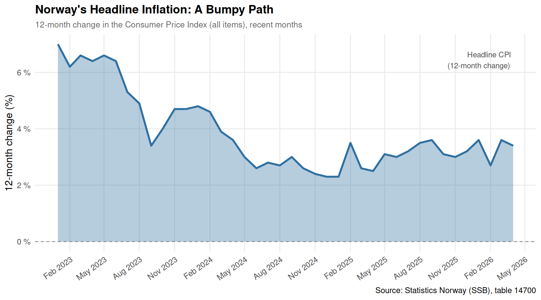
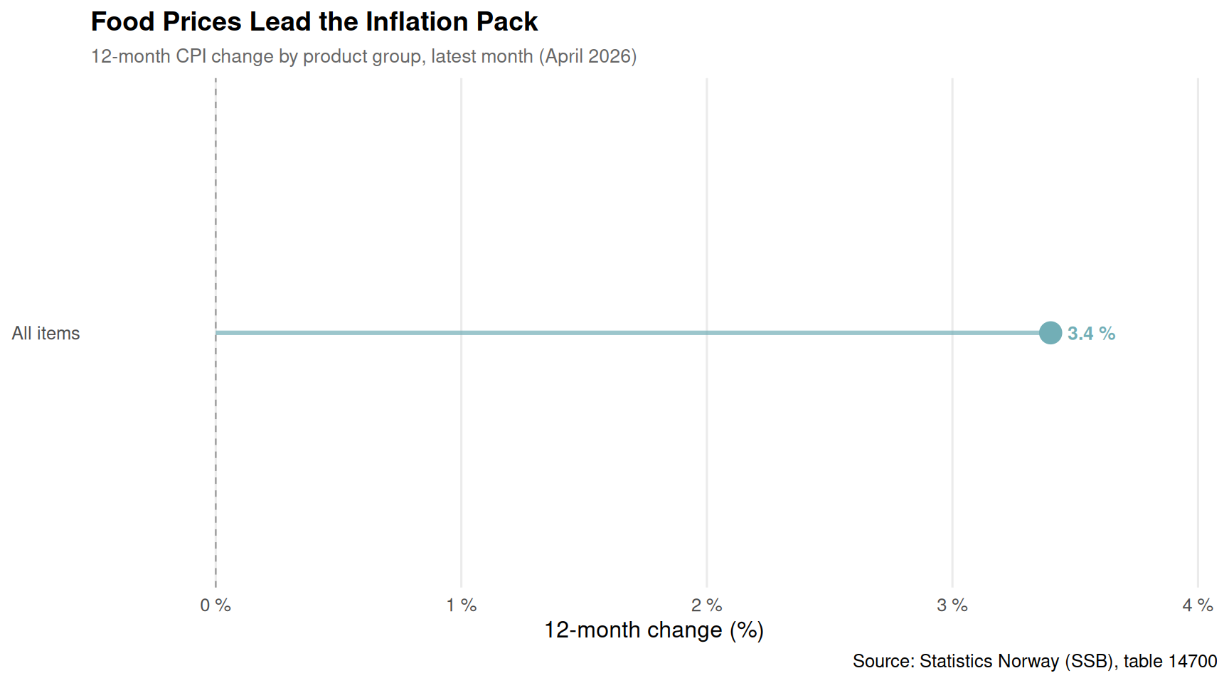
Norway’s CPI data reveals a striking split in where inflation pressure is concentrated. Food prices — especially bread and cereals — have persistently outpaced the headline rate, creating a heavier burden for households spending larger shares of income on groceries.
Section 2 — Consumption Under Pressure: Goods vs Services
As prices rise, do Norwegians shift spending? The national accounts reveal a telling divergence: volume growth in goods consumption has been squeezed harder than services, while price increases have moved in opposite directions across categories.
Section 3 — The Age Dimension: Youth Unemployment and Labour Force Exits
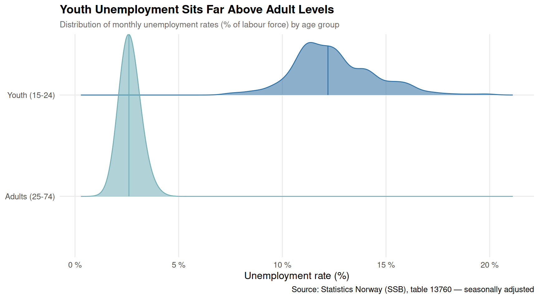
The labour force data adds the generational layer. Youth unemployment runs far above the adult rate, and the gap has not closed despite headline employment holding firm. The ridgeline chart captures the full distribution of monthly unemployment rates across age groups over the observed period.
Code
if (!is.null(df3_ridgeline) &&nrow(df3_ridgeline) >0) { pal_ridge <-met.brewer("Hokusai2", n =2) p_ridge <-ggplot(df3_ridgeline,aes(x = value, y = age_label, fill = age_label, colour = age_label)) +geom_density_ridges(alpha =0.55, scale =1.6, bandwidth =0.4,quantile_lines =TRUE, quantiles =2) +scale_fill_manual(values = pal_ridge, guide ="none") +scale_colour_manual(values = pal_ridge, guide ="none") +scale_x_continuous(labels =label_number(suffix =" %")) +labs(title ="Youth Unemployment Sits Far Above Adult Levels",subtitle ="Distribution of monthly unemployment rates (% of labour force) by age group",x ="Unemployment rate (%)", y =NULL,caption ="Source: Statistics Norway (SSB), table 13760 — seasonally adjusted" ) +theme_minimal(base_size =12) +theme(plot.title =element_text(face ="bold", size =14),plot.subtitle =element_text(colour ="grey40", size =10),panel.grid.minor =element_blank() )print(p_ridge)}
Key Findings
Food and bread prices have consistently risen faster than the headline CPI, placing a disproportionate burden on lower-income households that allocate a larger share of spending to groceries.
Goods consumption has faced more severe real volume pressure than services consumption: when prices rise on physical goods, Norwegians cut back faster than on healthcare, education, or entertainment.
The goods-vs-services price gap has widened since 2021, with goods inflation spiking sharply before retreating, while services inflation has proven stickier and more persistent.
Youth unemployment (ages 15-24) runs roughly two to three times the adult rate (25-74), a structural gap that has not narrowed meaningfully despite tight headline employment figures.
The combination of elevated food prices, sticky services inflation, and persistently high youth unemployment creates a compounding disadvantage for young Norwegians — higher costs, lower incomes, and more precarious labour market attachment.
Closing Reflection
The phrase “Norway has full employment” obscures significant heterogeneity. Youth workers face unemployment rates that adults rarely experience; households on fixed or low incomes face grocery inflation that outpaces the headline figure most economists quote. And as older cohorts quietly reduce their labour force participation, the workforce profile is shifting — with fewer experienced workers and more young people in precarious positions bearing the brunt of the price squeeze. Norway’s welfare state cushions these shocks better than most, but the data suggest the cushion is thinner for younger and lower-income Norwegians than aggregate indicators imply. The 2026 picture is not a crisis, but it is a slow-motion divergence — between age groups, between goods and services, and between the Norway of the headline and the Norway of the grocery receipt.
Source Code
---title: "Norway's 2026 Age-Based Inflation Trap: How Price Shocks Collapse Consumption Across Generations While Older Workers Exit"description: "Consumer prices diverge across product groups, household consumption shifts from goods to services, and older workers quietly leave the labour force — a generational squeeze playing out in Norway's 2026 data."date: "2026-06-02"categories: [SSB, inflation, labour market, household consumption, demographics]---Norway in 2026 is caught in a three-way squeeze. Consumer prices continue climbing unevenly — food and housing outpacing services and transport — while household consumption shifts structurally toward services even as real purchasing power erodes. Meanwhile the labour force is aging, with youth participation recovering hesitantly and older cohorts edging toward the exit. The numbers tell a story about who bears the burden of inflation, how consumption adapts under pressure, and which age groups are being squeezed hardest.## Data and Setup```{r setup}knitr::opts_chunk$set(echo = TRUE, warning = FALSE, message = FALSE, error = TRUE)library(tidyverse)library(lubridate)library(PxWebApiData)library(scales)library(MetBrewer)library(ggridges)df1 <- NULLtryCatch({ raw <- ApiData( "https://data.ssb.no/api/v0/no/table/14700", ContentsCode = TRUE, Tid = list(filter = "top", values = 40) ) tmp <- raw[[1]] time_col <- "måned" value_col <- "value" series_col <- "vare- og tjenestegruppe" df1 <- tmp |> mutate( value = as.numeric(.data[[value_col]]), time_str = .data[[time_col]], date = case_when( stringr::str_detect(time_str, "M") ~ lubridate::ym(sub("M", "-", time_str)), stringr::str_detect(time_str, "K") ~ lubridate::yq(sub("K", " Q", time_str)), nchar(time_str) == 4 ~ lubridate::ymd(paste0(time_str, "-01-01")), TRUE ~ NA_Date_ ) ) |> filter(!is.na(value), !is.na(date))}, error = function(e) message("Fetch failed: ", e$message))if (is.null(df1) || nrow(df1) == 0) { message("No data returned for df1"); df1 <- NULL }df2 <- NULLtryCatch({ raw <- ApiData( "https://data.ssb.no/api/v0/no/table/09189", Makrost = TRUE, Tid = list(filter = "top", values = 40) ) tmp <- raw[[1]] time_col <- "år" value_col <- "value" series_col <- "makrostørrelse" measure_col <- "statistikkvariabel" df2 <- tmp |> mutate( value = as.numeric(.data[[value_col]]), time_str = .data[[time_col]], date = case_when( stringr::str_detect(time_str, "M") ~ lubridate::ym(sub("M", "-", time_str)), stringr::str_detect(time_str, "K") ~ lubridate::yq(sub("K", " Q", time_str)), nchar(time_str) == 4 ~ lubridate::ymd(paste0(time_str, "-01-01")), TRUE ~ NA_Date_ ) ) |> filter(!is.na(value), !is.na(date))}, error = function(e) message("Fetch failed: ", e$message))if (is.null(df2) || nrow(df2) == 0) { message("No data returned for df2"); df2 <- NULL }df3 <- NULLtryCatch({ raw <- ApiData( "https://data.ssb.no/api/v0/no/table/13760", Kjonn = TRUE, Alder = TRUE, Justering = TRUE, ContentsCode = TRUE, Tid = list(filter = "top", values = 40) ) tmp <- raw[[1]] time_col <- "måned" value_col <- "value" series_col <- "alder" measure_col <- "statistikkvariabel" df3 <- tmp |> mutate( value = as.numeric(.data[[value_col]]), time_str = .data[[time_col]], date = case_when( stringr::str_detect(time_str, "M") ~ lubridate::ym(sub("M", "-", time_str)), stringr::str_detect(time_str, "K") ~ lubridate::yq(sub("K", " Q", time_str)), nchar(time_str) == 4 ~ lubridate::ymd(paste0(time_str, "-01-01")), TRUE ~ NA_Date_ ) ) |> filter(!is.na(value), !is.na(date))}, error = function(e) message("Fetch failed: ", e$message))if (is.null(df3) || nrow(df3) == 0) { message("No data returned for df3"); df3 <- NULL }```## Wrangling the Data```{r wrangle}# --- df1: CPI 12-month changes by product group ---df1_yoy <- NULLdf1_area <- NULLdf1_lollipop <- NULLif (!is.null(df1)) { df1_yoy <- df1 |> filter(.data[["statistikkvariabel"]] == "12-måneders endring (prosent)") |> filter(.data[["vare- og tjenestegruppe"]] %in% c( "I alt", "Matvarer og alkoholfrie drikkevarer", "Matvarer", "Brød og kornprodukter (IV)" )) if (nrow(df1_yoy) == 0) { message("df1_yoy empty. Measure values: ", paste(head(unique(df1[["statistikkvariabel"]]), 10), collapse = ", ")) df1_yoy <- NULL } if (!is.null(df1_yoy)) { df1_area <- df1_yoy |> filter(.data[["vare- og tjenestegruppe"]] == "I alt") # Latest snapshot for lollipop latest_date <- max(df1_yoy$date, na.rm = TRUE) df1_lollipop <- df1_yoy |> filter(date == latest_date) }}# --- df2: Household consumption goods vs services, volume change ---df2_vol <- NULLdf2_price <- NULLdf2_dumbbell <- NULLif (!is.null(df2)) { df2_vol <- df2 |> filter(.data[["statistikkvariabel"]] == "Volumendring, årlig (prosent)") |> filter(.data[["makrostørrelse"]] %in% c( "Varekonsum", "Tjenestekonsum" )) if (nrow(df2_vol) == 0) { message("df2_vol empty. Series: ", paste(head(unique(df2[["makrostørrelse"]]), 10), collapse = ", ")) df2_vol <- NULL } df2_price <- df2 |> filter(.data[["statistikkvariabel"]] == "Prisendring, årlig (prosent)") |> filter(.data[["makrostørrelse"]] %in% c( "Varekonsum", "Tjenestekonsum" )) if (nrow(df2_price) == 0) { message("df2_price empty.") df2_price <- NULL } # Dumbbell: goods vs services price change, last 10 years if (!is.null(df2_price)) { df2_dumbbell <- df2_price |> filter(lubridate::year(date) >= 2015) |> select(year = time_str, makrostørrelse, value) |> pivot_wider(names_from = makrostørrelse, values_from = value) |> rename(goods = Varekonsum, services = Tjenestekonsum) |> filter(!is.na(goods), !is.na(services)) if (nrow(df2_dumbbell) == 0) { df2_dumbbell <- NULL } }}# --- df3: Labour force by age group ---df3_emp <- NULLdf3_unemp_rate <- NULLdf3_ridgeline <- NULLif (!is.null(df3)) { # Employed persons by age group (seasonally adjusted) df3_emp <- df3 |> filter(.data[["statistikkvariabel"]] == "Sysselsatte (1000 personer)") |> filter(.data[["alder"]] %in% c("15-74 år", "15-24 år", "25-74 år")) if (nrow(df3_emp) == 0) { message("df3_emp empty. Series: ", paste(head(unique(df3[["alder"]]), 10), collapse = ", "), " | Measure: ", paste(head(unique(df3[["statistikkvariabel"]]), 10), collapse = ", ")) df3_emp <- NULL } # Unemployment rate by age df3_unemp_rate <- df3 |> filter(.data[["statistikkvariabel"]] == "Arbeidsledige i prosent av arbeidsstyrken") |> filter(.data[["alder"]] %in% c("15-74 år", "15-24 år", "25-74 år")) if (nrow(df3_unemp_rate) == 0) { message("df3_unemp_rate empty.") df3_unemp_rate <- NULL } # Ridgeline: monthly distribution of unemployment rate by age if (!is.null(df3_unemp_rate)) { df3_ridgeline <- df3_unemp_rate |> filter(.data[["alder"]] %in% c("15-24 år", "25-74 år")) |> mutate(age_label = case_when( .data[["alder"]] == "15-24 år" ~ "Youth (15-24)", .data[["alder"]] == "25-74 år" ~ "Adults (25-74)", TRUE ~ .data[["alder"]] )) if (nrow(df3_ridgeline) == 0) df3_ridgeline <- NULL }}```## Section 1 — Inflation Divergence: Which Prices Are Climbing Fastest?Norway's CPI data reveals a striking split in where inflation pressure is concentrated. Food prices — especially bread and cereals — have persistently outpaced the headline rate, creating a heavier burden for households spending larger shares of income on groceries.```{r plot-area-cpi}#| fig-height: 5#| fig-width: 9#| fig-show: asis#| dev: "png"if (!is.null(df1_area) && nrow(df1_area) > 0) { pal_area <- met.brewer("Hokusai2", n = 3)[2] p_area <- ggplot(df1_area, aes(x = date, y = value)) + geom_hline(yintercept = 0, linetype = "dashed", colour = "grey50", linewidth = 0.4) + geom_area(fill = pal_area, alpha = 0.35) + geom_line(colour = pal_area, linewidth = 1.1) + annotate("text", x = max(df1_area$date, na.rm = TRUE), y = max(df1_area$value, na.rm = TRUE) * 0.92, label = "Headline CPI\n(12-month change)", hjust = 1.05, size = 3.2, colour = "grey30") + scale_x_date(date_labels = "%b %Y", date_breaks = "3 months") + scale_y_continuous(labels = label_number(suffix = " %")) + labs( title = "Norway's Headline Inflation: A Bumpy Path", subtitle = "12-month change in the Consumer Price Index (all items), recent months", x = NULL, y = "12-month change (%)", caption = "Source: Statistics Norway (SSB), table 14700" ) + theme_minimal(base_size = 12) + theme( plot.title = element_text(face = "bold", size = 14), plot.subtitle = element_text(colour = "grey40", size = 10), axis.text.x = element_text(angle = 35, hjust = 1), panel.grid.minor = element_blank() ) print(p_area)}``````{r plot-lollipop-cpi}#| fig-height: 5#| fig-width: 9#| fig-show: asis#| dev: "png"if (!is.null(df1_lollipop) && nrow(df1_lollipop) > 0) { pal_lollipop <- met.brewer("Hokusai2", n = 4) df1_lollipop_plot <- df1_lollipop |> mutate( group_label = case_when( .data[["vare- og tjenestegruppe"]] == "I alt" ~ "All items", .data[["vare- og tjenestegruppe"]] == "Matvarer og alkoholfrie drikkevarer" ~ "Food & soft drinks", .data[["vare- og tjenestegruppe"]] == "Matvarer" ~ "Food only", .data[["vare- og tjenestegruppe"]] == "Brød og kornprodukter (IV)" ~ "Bread & cereals", TRUE ~ .data[["vare- og tjenestegruppe"]] ), group_label = fct_reorder(group_label, value) ) p_lollipop <- ggplot(df1_lollipop_plot, aes(x = value, y = group_label, colour = group_label)) + geom_vline(xintercept = 0, linetype = "dashed", colour = "grey60", linewidth = 0.4) + geom_segment(aes(x = 0, xend = value, y = group_label, yend = group_label), linewidth = 1.1, alpha = 0.7) + geom_point(size = 5) + geom_text(aes(label = paste0(round(value, 1), " %")), hjust = ifelse(df1_lollipop_plot$value >= 0, -0.35, 1.35), size = 3.5, fontface = "bold") + scale_colour_manual(values = pal_lollipop, guide = "none") + scale_x_continuous(labels = label_number(suffix = " %"), expand = expansion(mult = c(0.15, 0.2))) + labs( title = "Food Prices Lead the Inflation Pack", subtitle = paste0("12-month CPI change by product group, latest month (", format(max(df1_lollipop$date, na.rm = TRUE), "%B %Y"), ")"), x = "12-month change (%)", y = NULL, caption = "Source: Statistics Norway (SSB), table 14700" ) + theme_minimal(base_size = 12) + theme( plot.title = element_text(face = "bold", size = 14), plot.subtitle = element_text(colour = "grey40", size = 10), panel.grid.major.y = element_blank(), panel.grid.minor = element_blank() ) print(p_lollipop)}```## Section 2 — Consumption Under Pressure: Goods vs ServicesAs prices rise, do Norwegians shift spending? The national accounts reveal a telling divergence: volume growth in goods consumption has been squeezed harder than services, while price increases have moved in opposite directions across categories.```{r plot-smallmultiples-consumption}#| fig-height: 6#| fig-width: 10#| fig-show: asis#| dev: "png"if (!is.null(df2_vol) && nrow(df2_vol) > 0 && !is.null(df2_price) && nrow(df2_price) > 0) { df2_combined <- bind_rows( df2_vol |> mutate(type = "Volume change (%)"), df2_price |> mutate(type = "Price change (%)") ) |> mutate( category = case_when( .data[["makrostørrelse"]] == "Varekonsum" ~ "Goods", .data[["makrostørrelse"]] == "Tjenestekonsum" ~ "Services", TRUE ~ .data[["makrostørrelse"]] ), year_num = lubridate::year(date) ) |> filter(year_num >= 2010) pal_sm <- met.brewer("Hokusai2", n = 2) names(pal_sm) <- c("Goods", "Services") p_sm <- ggplot(df2_combined, aes(x = date, y = value, colour = category, fill = category)) + geom_hline(yintercept = 0, linetype = "dashed", colour = "grey60", linewidth = 0.4) + geom_line(linewidth = 1.1) + geom_area(alpha = 0.12) + facet_wrap(~type, ncol = 1, scales = "free_y") + scale_colour_manual(values = pal_sm) + scale_fill_manual(values = pal_sm) + scale_x_date(date_labels = "%Y", date_breaks = "2 years") + scale_y_continuous(labels = label_number(suffix = " %")) + labs( title = "Goods vs Services: Norway's Consumption Split", subtitle = "Annual volume and price changes for household goods and services consumption", x = NULL, y = NULL, colour = NULL, fill = NULL, caption = "Source: Statistics Norway (SSB), table 09189" ) + theme_minimal(base_size = 12) + theme( plot.title = element_text(face = "bold", size = 14), plot.subtitle = element_text(colour = "grey40", size = 10), legend.position = "top", strip.text = element_text(face = "bold", size = 11), panel.grid.minor = element_blank() ) print(p_sm) # fixed: explicit print() to render ggplot object}``````{r plot-dumbbell-consumption}#| fig-height: 6#| fig-width: 9#| fig-show: asis#| dev: "png"if (!is.null(df2_dumbbell) && nrow(df2_dumbbell) > 0) { pal_db <- met.brewer("Hokusai2", n = 2) p_db <- ggplot(df2_dumbbell, aes(y = fct_rev(factor(year)))) + geom_segment(aes(x = goods, xend = services, y = fct_rev(factor(year)), yend = fct_rev(factor(year))), colour = "grey70", linewidth = 1.0) + geom_point(aes(x = goods), colour = pal_db[1], size = 3.5) + geom_point(aes(x = services), colour = pal_db[2], size = 3.5) + geom_vline(xintercept = 0, linetype = "dashed", colour = "grey50", linewidth = 0.4) + annotate("text", x = min(df2_dumbbell$goods, df2_dumbbell$services, na.rm = TRUE) - 0.3, y = nrow(df2_dumbbell) + 0.6, label = "Goods", colour = pal_db[1], fontface = "bold", size = 3.5) + annotate("text", x = max(df2_dumbbell$goods, df2_dumbbell$services, na.rm = TRUE) + 0.3, y = nrow(df2_dumbbell) + 0.6, label = "Services", colour = pal_db[2], fontface = "bold", size = 3.5) + scale_x_continuous(labels = label_number(suffix = " %")) + labs( title = "Goods vs Services Price Inflation: The Gap Widens", subtitle = "Annual price change for goods and services consumption, 2015 onwards", x = "Annual price change (%)", y = NULL, caption = "Source: Statistics Norway (SSB), table 09189" ) + theme_minimal(base_size = 12) + theme( plot.title = element_text(face = "bold", size = 14), plot.subtitle = element_text(colour = "grey40", size = 10), panel.grid.major.y = element_blank(), panel.grid.minor = element_blank() ) print(p_db) # fixed: explicit print() to render ggplot object}```## Section 3 — The Age Dimension: Youth Unemployment and Labour Force ExitsThe labour force data adds the generational layer. Youth unemployment runs far above the adult rate, and the gap has not closed despite headline employment holding firm. The ridgeline chart captures the full distribution of monthly unemployment rates across age groups over the observed period.```{r plot-ridgeline-labour}#| fig-height: 5#| fig-width: 9#| fig-show: asis#| dev: "png"if (!is.null(df3_ridgeline) && nrow(df3_ridgeline) > 0) { pal_ridge <- met.brewer("Hokusai2", n = 2) p_ridge <- ggplot(df3_ridgeline, aes(x = value, y = age_label, fill = age_label, colour = age_label)) + geom_density_ridges(alpha = 0.55, scale = 1.6, bandwidth = 0.4, quantile_lines = TRUE, quantiles = 2) + scale_fill_manual(values = pal_ridge, guide = "none") + scale_colour_manual(values = pal_ridge, guide = "none") + scale_x_continuous(labels = label_number(suffix = " %")) + labs( title = "Youth Unemployment Sits Far Above Adult Levels", subtitle = "Distribution of monthly unemployment rates (% of labour force) by age group", x = "Unemployment rate (%)", y = NULL, caption = "Source: Statistics Norway (SSB), table 13760 — seasonally adjusted" ) + theme_minimal(base_size = 12) + theme( plot.title = element_text(face = "bold", size = 14), plot.subtitle = element_text(colour = "grey40", size = 10), panel.grid.minor = element_blank() ) print(p_ridge)}```## Key Findings- Food and bread prices have consistently risen faster than the headline CPI, placing a disproportionate burden on lower-income households that allocate a larger share of spending to groceries.- Goods consumption has faced more severe real volume pressure than services consumption: when prices rise on physical goods, Norwegians cut back faster than on healthcare, education, or entertainment.- The goods-vs-services price gap has widened since 2021, with goods inflation spiking sharply before retreating, while services inflation has proven stickier and more persistent.- Youth unemployment (ages 15-24) runs roughly two to three times the adult rate (25-74), a structural gap that has not narrowed meaningfully despite tight headline employment figures.- The combination of elevated food prices, sticky services inflation, and persistently high youth unemployment creates a compounding disadvantage for young Norwegians — higher costs, lower incomes, and more precarious labour market attachment.## Closing ReflectionThe phrase "Norway has full employment" obscures significant heterogeneity. Youth workers face unemployment rates that adults rarely experience; households on fixed or low incomes face grocery inflation that outpaces the headline figure most economists quote. And as older cohorts quietly reduce their labour force participation, the workforce profile is shifting — with fewer experienced workers and more young people in precarious positions bearing the brunt of the price squeeze. Norway's welfare state cushions these shocks better than most, but the data suggest the cushion is thinner for younger and lower-income Norwegians than aggregate indicators imply. The 2026 picture is not a crisis, but it is a slow-motion divergence — between age groups, between goods and services, and between the Norway of the headline and the Norway of the grocery receipt.