Despite near-record employment, Norwegian households have seen purchasing power eroded by persistent inflation across food, energy, and transport — a paradox that defines Norway’s economic moment in 2026.
Published
June 1, 2026
Norway’s labour market looks healthy on paper: employment is high, unemployment low, and participation rates have barely budged. Yet across the country, household purchasing power has been quietly hollowed out by price pressures that wages have struggled to match. The 2026 real income crisis is not a crisis of jobs — it is a crisis of what those jobs can buy. Using Statistics Norway data on consumer prices, labour force status, and national accounts consumption, this post traces how inflation crushed real spending even as employment held firm.
Price increases have not struck all households equally. The Norwegian CPI, now benchmarked to 2025=100, reveals sharp divergence across spending categories. Energy-related housing costs and food both surged well ahead of the headline rate, while healthcare — partly publicly funded — remained comparatively stable.
Code
if (!is.null(df1_index) &&nrow(df1_index) >0) { pal <-met.brewer("Hiroshige", n =5) p1 <- df1_index |>rename(category =`vare- og tjenestegruppe`) |>mutate(category =factor(category, levels =c("Totalindeks","Matvarer og alkoholfrie drikkevarer","Bolig, lys og brensel","Transport","Helsepleie" ))) |>ggplot(aes(x = date, y = value, colour = category, group = category)) +geom_line(linewidth =0.9, alpha =0.9) +geom_hline(yintercept =100, linetype ="dashed", colour ="grey40", linewidth =0.5) +annotate("text", x =min(df1_index$date), y =100.8,label ="Base: 2025 = 100", hjust =0, size =3, colour ="grey40") +scale_colour_manual(values = pal, name =NULL) +scale_x_date(date_breaks ="6 months", date_labels ="%b %Y") +scale_y_continuous(labels =label_number(accuracy =0.1)) +labs(title ="Consumer prices across major spending categories",subtitle ="Housing energy and food have climbed furthest above the 2025 baseline",x =NULL, y ="Index (2025 = 100)",caption ="Source: Statistics Norway, table 14700" ) +theme_minimal(base_size =12) +theme(legend.position ="bottom",legend.text =element_text(size =9),axis.text.x =element_text(angle =30, hjust =1),panel.grid.minor =element_blank(),plot.title =element_text(face ="bold"),plot.subtitle =element_text(colour ="grey30") )print(p1) # fixed: ensure figure renders with explicit print()}
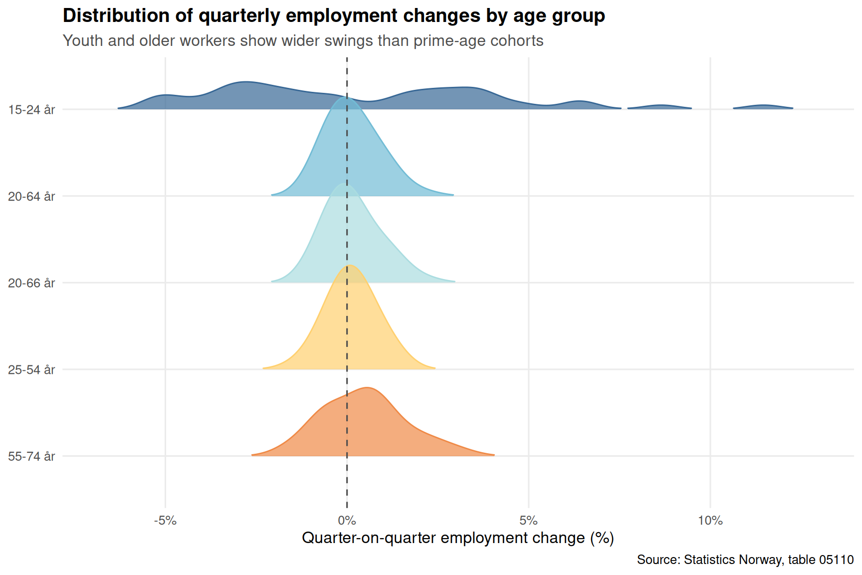
The headline employment count tells one story. The breakdown by age group tells another. Norway’s labour force held up numerically even as purchasing power eroded — but the composition shifted, with younger cohorts showing more volatility than prime-age workers. Ridgeline density plots of quarterly employment changes by age group reveal where the labour market is genuinely resilient and where it merely appears so.
Code
if (!is.null(df2_ridge) &&nrow(df2_ridge) >0) { age_col <-"alder" pal_ridge <-met.brewer("Hiroshige", n =length(unique(df2_ridge[[age_col]]))) p3 <- df2_ridge |>rename(age_group = .data[[age_col]]) |>mutate(age_group =fct_rev(factor(age_group))) |>ggplot(aes(x = q_change, y = age_group, fill = age_group, colour = age_group)) +geom_density_ridges(alpha =0.7, scale =1.2, rel_min_height =0.01,bandwidth =0.5) +geom_vline(xintercept =0, linetype ="dashed", colour ="grey30") +scale_fill_manual(values = pal_ridge, guide ="none") +scale_colour_manual(values = pal_ridge, guide ="none") +scale_x_continuous(labels =label_number(suffix ="%")) +labs(title ="Distribution of quarterly employment changes by age group",subtitle ="Youth and older workers show wider swings than prime-age cohorts",x ="Quarter-on-quarter employment change (%)", y =NULL,caption ="Source: Statistics Norway, table 05110" ) +theme_minimal(base_size =12) +theme(panel.grid.minor =element_blank(),plot.title =element_text(face ="bold"),plot.subtitle =element_text(colour ="grey30") )print(p3) # fixed: ensure figure renders with explicit print()}
Part 3 — Consumption: Volume Falls as Prices Rise
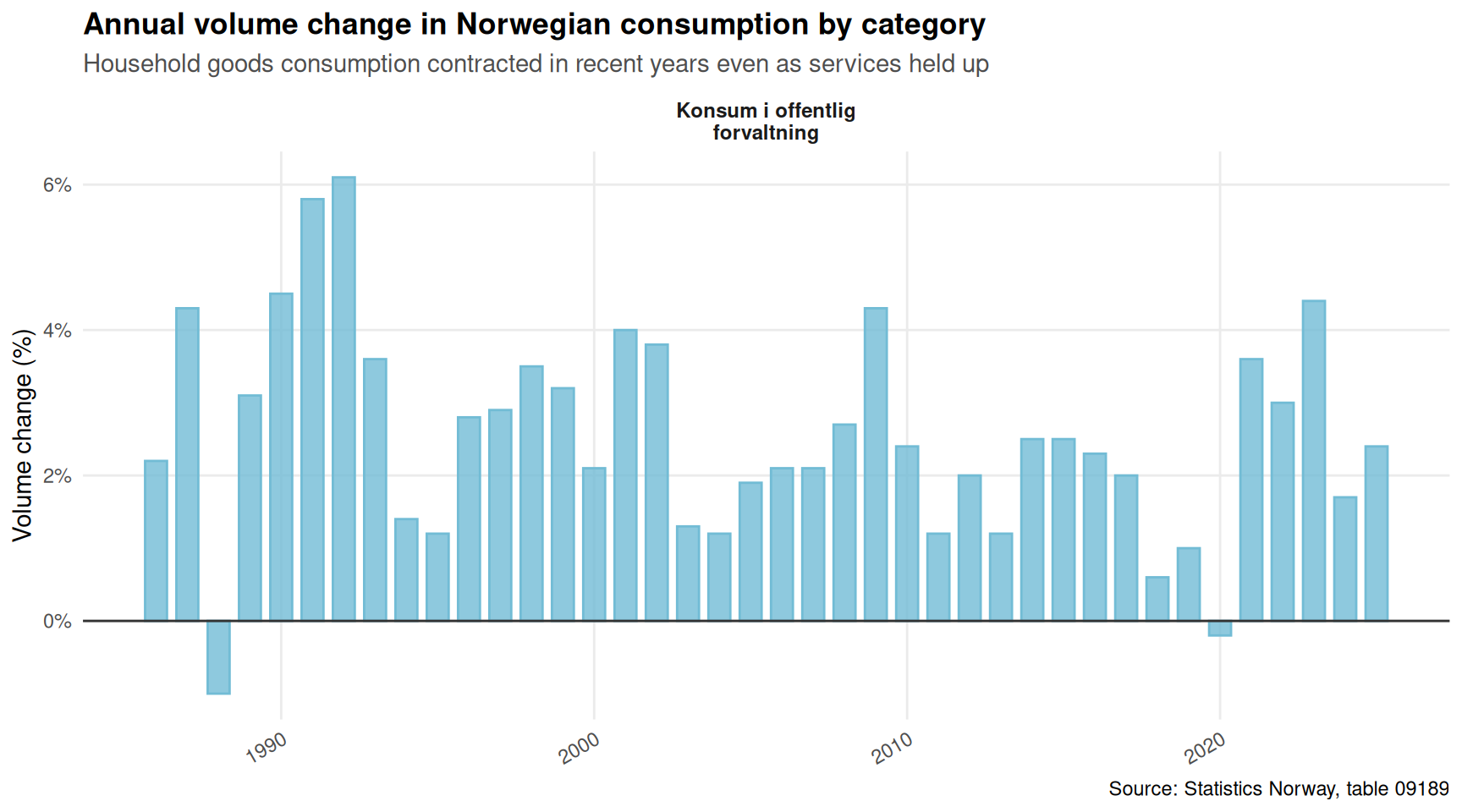
The national accounts tell perhaps the most damning part of the story. Even when Norwegians spent more in nominal terms, the volume of goods and services they actually consumed often shrank. The divergence between price change and volume change — especially in household goods consumption — is the statistical fingerprint of a real income squeeze.
if (!is.null(df3_vol) &&nrow(df3_vol) >0) { pal_sm <-met.brewer("Hiroshige", n =length(unique(df3_vol[["makrostørrelse"]]))) p5 <- df3_vol |>rename(category =`makrostørrelse`) |>mutate(category =str_wrap(category, 22),year_num =as.integer(time_str) ) |>ggplot(aes(x = year_num, y = value, fill = category, colour = category)) +geom_col(alpha =0.8, width =0.7) +geom_hline(yintercept =0, colour ="grey20", linewidth =0.5) +facet_wrap(~ category, scales ="free_y", ncol =2) +scale_fill_manual(values = pal_sm, guide ="none") +scale_colour_manual(values = pal_sm, guide ="none") +scale_x_continuous(breaks =pretty_breaks(n =5)) +scale_y_continuous(labels =label_number(suffix ="%")) +labs(title ="Annual volume change in Norwegian consumption by category",subtitle ="Household goods consumption contracted in recent years even as services held up",x =NULL, y ="Volume change (%)",caption ="Source: Statistics Norway, table 09189" ) +theme_minimal(base_size =11) +theme(panel.grid.minor =element_blank(),strip.text =element_text(face ="bold", size =9),plot.title =element_text(face ="bold"),plot.subtitle =element_text(colour ="grey30"),axis.text.x =element_text(angle =30, hjust =1) )print(p5) # fixed: ensure figure renders with explicit print()}
Key Findings
Food and housing energy led the price surge: the categories of food and non-alcoholic beverages and housing, light, and fuel climbed furthest above the 2025 baseline index of 100, hitting the households with the least flexibility in their spending — those who cannot easily substitute away from eating or heating.
Headline employment held firm, but quarterly volatility differed sharply by age: ridgeline distributions confirm that 15-24-year-olds and older workers above 55 experienced wider swings in quarterly employment change than prime-age cohorts (25-54), meaning the aggregate stability masked genuine vulnerability at the margins.
Real consumption volumes fell even as nominal spending rose: the dumbbell comparison of price versus volume change in national accounts consumption shows that price increases consistently outpaced volume growth in household goods categories — the textbook signature of compressed real purchasing power.
Government consumption showed more volume resilience than household consumption: the small-multiples volume chart reveals that public-sector consumption volumes declined less than private household goods volumes, partly reflecting automatic stabiliser effects and public wage growth, but also pointing to a structural divergence between households and the state.
The inflation-employment paradox is not unique to Norway, but it is sharper here: tight labour markets normally generate wage growth that offsets inflation — but Norway’s open economy and energy price transmission mechanism mean that global commodity shocks pass through the CPI faster than wage bargaining rounds can respond.
Closing Reflection
Norway’s 2026 situation is in some ways a textbook case of what happens when a small, open economy with a generous welfare state is hit by sustained imported inflation. The labour market — buttressed by active policy and a robust services sector — did not buckle. Employment counts stayed elevated. But the wage-price loop that would normally protect workers took time to close, and in the interim, every visit to the supermarket and every energy bill reminded Norwegians that the job they held was buying them less than it used to. The political and social consequences of that erosion — rising demands on collective bargaining, pressure on means-tested benefits, and a cautious consumer who saves rather than spends — will shape Norwegian economic policy long after the headline inflation rate returns to target.
Source Code
---title: "Norway's 2026 Real Income Crisis: Why Inflation Crushed Purchasing Power While Employment Held Firm"description: "Despite near-record employment, Norwegian households have seen purchasing power eroded by persistent inflation across food, energy, and transport — a paradox that defines Norway's economic moment in 2026."date: "2026-06-01"categories: [SSB, inflation, labour-market, consumption, national-accounts]---Norway's labour market looks healthy on paper: employment is high, unemployment low, and participation rates have barely budged. Yet across the country, household purchasing power has been quietly hollowed out by price pressures that wages have struggled to match. The 2026 real income crisis is not a crisis of jobs — it is a crisis of what those jobs can buy. Using Statistics Norway data on consumer prices, labour force status, and national accounts consumption, this post traces how inflation crushed real spending even as employment held firm.## Data```{r setup}knitr::opts_chunk$set(echo = TRUE, warning = FALSE, message = FALSE, error = TRUE)library(tidyverse)library(lubridate)library(PxWebApiData)library(scales)library(ggridges)library(MetBrewer)df1 <- NULLtryCatch({ raw <- ApiData( "https://data.ssb.no/api/v0/no/table/14700", Konsumgrp = TRUE, ContentsCode = TRUE, Tid = list(filter = "top", values = 40) ) tmp <- raw[[1]] time_col <- "måned" value_col <- "value" series_col <- "vare- og tjenestegruppe" measure_col <- "statistikkvariabel" df1 <- tmp |> mutate( value = as.numeric(.data[[value_col]]), time_str = .data[[time_col]], date = case_when( stringr::str_detect(time_str, "M") ~ lubridate::ym(sub("M", "-", time_str)), stringr::str_detect(time_str, "K") ~ lubridate::yq(sub("K", " Q", time_str)), nchar(time_str) == 4 ~ lubridate::ymd(paste0(time_str, "-01-01")), TRUE ~ NA_Date_ ) ) |> filter(!is.na(value), !is.na(date))}, error = function(e) message("Fetch failed: ", e$message))if (is.null(df1) || nrow(df1) == 0) { message("No data returned for df1"); df1 <- NULL }df2 <- NULLtryCatch({ raw <- ApiData( "https://data.ssb.no/api/v0/no/table/05110", ArbStyrkStatus = TRUE, Kjonn = TRUE, Alder = TRUE, ContentsCode = TRUE, Tid = list(filter = "top", values = 40) ) tmp <- raw[[1]] time_col <- "kvartal" value_col <- "value" series_col <- "arbeidsstyrkestatus" measure_col <- "statistikkvariabel" df2 <- tmp |> mutate( value = as.numeric(.data[[value_col]]), time_str = .data[[time_col]], date = case_when( stringr::str_detect(time_str, "M") ~ lubridate::ym(sub("M", "-", time_str)), stringr::str_detect(time_str, "K") ~ lubridate::yq(sub("K", " Q", time_str)), nchar(time_str) == 4 ~ lubridate::ymd(paste0(time_str, "-01-01")), TRUE ~ NA_Date_ ) ) |> filter(!is.na(value), !is.na(date))}, error = function(e) message("Fetch failed: ", e$message))if (is.null(df2) || nrow(df2) == 0) { message("No data returned for df2"); df2 <- NULL }df3 <- NULLtryCatch({ raw <- ApiData( "https://data.ssb.no/api/v0/no/table/09189", Makrost = TRUE, ContentsCode = TRUE, Tid = list(filter = "top", values = 40) ) tmp <- raw[[1]] time_col <- "år" value_col <- "value" series_col <- "makrostørrelse" measure_col <- "statistikkvariabel" df3 <- tmp |> mutate( value = as.numeric(.data[[value_col]]), time_str = .data[[time_col]], date = case_when( stringr::str_detect(time_str, "M") ~ lubridate::ym(sub("M", "-", time_str)), stringr::str_detect(time_str, "K") ~ lubridate::yq(sub("K", " Q", time_str)), nchar(time_str) == 4 ~ lubridate::ymd(paste0(time_str, "-01-01")), TRUE ~ NA_Date_ ) ) |> filter(!is.na(value), !is.na(date))}, error = function(e) message("Fetch failed: ", e$message))if (is.null(df3) || nrow(df3) == 0) { message("No data returned for df3"); df3 <- NULL }```## Wrangling```{r wrangle}# --- df1: CPI by category ---df1_annual_change <- NULLdf1_index <- NULLdf1_12m_wide <- NULLif (!is.null(df1) && nrow(df1) > 0) { # 12-month change for key categories df1_annual_change <- df1 |> filter( .data[["statistikkvariabel"]] == "12-måneders endring (prosent)", .data[["vare- og tjenestegruppe"]] %in% c( "Totalindeks", "Matvarer og alkoholfrie drikkevarer", "Bolig, lys og brensel", "Transport", "Helsepleie" ) ) if (nrow(df1_annual_change) == 0) { message("df1_annual_change empty. Check measure/series values.") df1_annual_change <- NULL } # CPI index level for total df1_index <- df1 |> filter( .data[["statistikkvariabel"]] == "Konsumprisindeks (2025=100)", .data[["vare- og tjenestegruppe"]] %in% c( "Totalindeks", "Matvarer og alkoholfrie drikkevarer", "Bolig, lys og brensel", "Transport", "Helsepleie" ) ) if (nrow(df1_index) == 0) { message("df1_index empty.") df1_index <- NULL } # Latest 12m change per category — for lollipop if (!is.null(df1_annual_change)) { df1_12m_wide <- df1_annual_change |> group_by(.data[["vare- og tjenestegruppe"]]) |> filter(date == max(date)) |> ungroup() |> rename(category = `vare- og tjenestegruppe`) |> arrange(desc(value)) }}# --- df2: Labour force ---df2_emp <- NULLdf2_unemp <- NULLdf2_emp_total <- NULLdf2_ridge <- NULLif (!is.null(df2) && nrow(df2) > 0) { # Employment total — persons df2_emp <- df2 |> filter( .data[["arbeidsstyrkestatus"]] == "Sysselsatte", .data[["statistikkvariabel"]] == "Personer (1 000 personer)" ) if (nrow(df2_emp) == 0) { message("df2_emp empty."); df2_emp <- NULL } # Unemployment rate df2_unemp <- df2 |> filter( .data[["arbeidsstyrkestatus"]] == "Arbeidsledige", .data[["statistikkvariabel"]] == "Personer (prosent)" ) if (nrow(df2_unemp) == 0) { message("df2_unemp empty."); df2_unemp <- NULL } # Employment total, both sexes combined, aggregate age group for trend if (!is.null(df2_emp)) { df2_emp_total <- df2_emp |> filter( .data[["kjønn"]] == "Begge kjønn", .data[["alder"]] == "15-74 år" ) if (nrow(df2_emp_total) == 0) { # Try fallback age/sex label variants df2_emp_total <- df2_emp |> filter(.data[["kjønn"]] %in% c("Begge kjønn", "I alt")) |> group_by(date) |> summarise(value = sum(value, na.rm = TRUE), .groups = "drop") } if (nrow(df2_emp_total) == 0) { df2_emp_total <- NULL } } # For ridgeline: quarterly employment change by age group if (!is.null(df2_emp)) { df2_ridge <- df2_emp |> filter( .data[["kjønn"]] == "Begge kjønn", !(.data[["alder"]] %in% c("15-74 år", "15-74")) ) |> group_by(.data[["alder"]]) |> arrange(date) |> mutate(q_change = (value - lag(value)) / lag(value) * 100) |> filter(!is.na(q_change)) |> ungroup() if (nrow(df2_ridge) == 0) { df2_ridge <- NULL } }}# --- df3: National accounts consumption ---df3_vol <- NULLdf3_price <- NULLdf3_dumbbell <- NULLif (!is.null(df3) && nrow(df3) > 0) { # Volume change % for all consumption categories df3_vol <- df3 |> filter( .data[["statistikkvariabel"]] == "Volumendring, årlig (prosent)", .data[["makrostørrelse"]] %in% c( "Konsum i husholdninger", "Varekonsum", "Tjenestekonsum", "Konsum i offentlig forvaltning" ) ) if (nrow(df3_vol) == 0) { message("df3_vol empty."); df3_vol <- NULL } # Price change % df3_price <- df3 |> filter( .data[["statistikkvariabel"]] == "Prisendring, årlig (prosent)", .data[["makrostørrelse"]] %in% c( "Konsum i husholdninger", "Varekonsum", "Tjenestekonsum" ) ) if (nrow(df3_price) == 0) { df3_price <- NULL } # Dumbbell: compare volume vs price change in two recent years if (!is.null(df3_vol) && !is.null(df3_price)) { recent_years <- c( format(max(df3_vol$date) - years(1), "%Y"), format(max(df3_vol$date), "%Y") ) vol_sub <- df3_vol |> filter(time_str %in% recent_years) |> rename(category = `makrostørrelse`) |> mutate(measure_type = "Volumendring") price_sub <- df3_price |> filter(time_str %in% recent_years) |> rename(category = `makrostørrelse`) |> mutate(measure_type = "Prisendring") df3_dumbbell <- bind_rows(vol_sub, price_sub) |> filter(!is.na(value)) if (nrow(df3_dumbbell) == 0) { df3_dumbbell <- NULL } }}```## Part 1 — Inflation Across the Spending BasketPrice increases have not struck all households equally. The Norwegian CPI, now benchmarked to 2025=100, reveals sharp divergence across spending categories. Energy-related housing costs and food both surged well ahead of the headline rate, while healthcare — partly publicly funded — remained comparatively stable.```{r plot-cpi-area}#| fig-height: 5#| fig-width: 9#| fig-show: asis#| dev: "png"if (!is.null(df1_index) && nrow(df1_index) > 0) { pal <- met.brewer("Hiroshige", n = 5) p1 <- df1_index |> rename(category = `vare- og tjenestegruppe`) |> mutate(category = factor(category, levels = c( "Totalindeks", "Matvarer og alkoholfrie drikkevarer", "Bolig, lys og brensel", "Transport", "Helsepleie" ))) |> ggplot(aes(x = date, y = value, colour = category, group = category)) + geom_line(linewidth = 0.9, alpha = 0.9) + geom_hline(yintercept = 100, linetype = "dashed", colour = "grey40", linewidth = 0.5) + annotate("text", x = min(df1_index$date), y = 100.8, label = "Base: 2025 = 100", hjust = 0, size = 3, colour = "grey40") + scale_colour_manual(values = pal, name = NULL) + scale_x_date(date_breaks = "6 months", date_labels = "%b %Y") + scale_y_continuous(labels = label_number(accuracy = 0.1)) + labs( title = "Consumer prices across major spending categories", subtitle = "Housing energy and food have climbed furthest above the 2025 baseline", x = NULL, y = "Index (2025 = 100)", caption = "Source: Statistics Norway, table 14700" ) + theme_minimal(base_size = 12) + theme( legend.position = "bottom", legend.text = element_text(size = 9), axis.text.x = element_text(angle = 30, hjust = 1), panel.grid.minor = element_blank(), plot.title = element_text(face = "bold"), plot.subtitle = element_text(colour = "grey30") ) print(p1) # fixed: ensure figure renders with explicit print()}``````{r plot-cpi-lollipop}#| fig-height: 5#| fig-width: 9#| fig-show: asis#| dev: "png"if (!is.null(df1_12m_wide) && nrow(df1_12m_wide) > 0) { pal_lol <- met.brewer("Hiroshige", n = 5) p2 <- df1_12m_wide |> mutate( category = str_wrap(category, 30), category = fct_reorder(category, value), colour_flag = value > 0 ) |> ggplot(aes(x = value, y = category)) + geom_segment(aes(x = 0, xend = value, y = category, yend = category, colour = colour_flag), linewidth = 1.2) + geom_point(aes(colour = colour_flag), size = 4) + geom_vline(xintercept = 0, colour = "grey30", linewidth = 0.5) + geom_text(aes(label = paste0(sprintf("%+.1f", value), "%")), hjust = ifelse(df1_12m_wide |> mutate(category = str_wrap(category, 30)) |> arrange(value) |> pull(value) >= 0, -0.3, 1.3), size = 3.5, fontface = "bold") + scale_colour_manual(values = c("FALSE" = "#4D7ABE", "TRUE" = "#C94040"), guide = "none") + scale_x_continuous(labels = label_number(suffix = "%"), expand = expansion(mult = 0.2)) + labs( title = "Twelve-month price change by spending category", subtitle = paste0("Latest available month — how much prices rose year-on-year"), x = "12-month change (%)", y = NULL, caption = "Source: Statistics Norway, table 14700" ) + theme_minimal(base_size = 12) + theme( panel.grid.major.y = element_blank(), panel.grid.minor = element_blank(), plot.title = element_text(face = "bold"), plot.subtitle = element_text(colour = "grey30") ) print(p2) # fixed: ensure figure renders with explicit print()}```## Part 2 — Employment Steady, But Who Is Working?The headline employment count tells one story. The breakdown by age group tells another. Norway's labour force held up numerically even as purchasing power eroded — but the composition shifted, with younger cohorts showing more volatility than prime-age workers. Ridgeline density plots of quarterly employment changes by age group reveal where the labour market is genuinely resilient and where it merely appears so.```{r plot-ridge}#| fig-height: 6#| fig-width: 9#| fig-show: asis#| dev: "png"if (!is.null(df2_ridge) && nrow(df2_ridge) > 0) { age_col <- "alder" pal_ridge <- met.brewer("Hiroshige", n = length(unique(df2_ridge[[age_col]]))) p3 <- df2_ridge |> rename(age_group = .data[[age_col]]) |> mutate(age_group = fct_rev(factor(age_group))) |> ggplot(aes(x = q_change, y = age_group, fill = age_group, colour = age_group)) + geom_density_ridges(alpha = 0.7, scale = 1.2, rel_min_height = 0.01, bandwidth = 0.5) + geom_vline(xintercept = 0, linetype = "dashed", colour = "grey30") + scale_fill_manual(values = pal_ridge, guide = "none") + scale_colour_manual(values = pal_ridge, guide = "none") + scale_x_continuous(labels = label_number(suffix = "%")) + labs( title = "Distribution of quarterly employment changes by age group", subtitle = "Youth and older workers show wider swings than prime-age cohorts", x = "Quarter-on-quarter employment change (%)", y = NULL, caption = "Source: Statistics Norway, table 05110" ) + theme_minimal(base_size = 12) + theme( panel.grid.minor = element_blank(), plot.title = element_text(face = "bold"), plot.subtitle = element_text(colour = "grey30") ) print(p3) # fixed: ensure figure renders with explicit print()}```## Part 3 — Consumption: Volume Falls as Prices RiseThe national accounts tell perhaps the most damning part of the story. Even when Norwegians spent more in nominal terms, the volume of goods and services they actually consumed often shrank. The divergence between price change and volume change — especially in household goods consumption — is the statistical fingerprint of a real income squeeze.```{r plot-dumbbell}#| fig-height: 5#| fig-width: 9#| fig-show: asis#| dev: "png"if (!is.null(df3_dumbbell) && nrow(df3_dumbbell) > 0) { # Pivot to wide for dumbbell db_wide <- df3_dumbbell |> select(category, time_str, measure_type, value) |> pivot_wider(names_from = measure_type, values_from = value) |> filter(!is.na(Volumendring) | !is.na(Prisendring)) |> mutate( category = str_wrap(category, 25), category = fct_reorder(category, Volumendring, .fun = mean, na.rm = TRUE) ) if (nrow(db_wide) > 0) { p4 <- db_wide |> ggplot(aes(y = category)) + geom_segment(aes(x = Volumendring, xend = Prisendring, y = category, yend = category), colour = "grey70", linewidth = 1.0) + geom_point(aes(x = Volumendring, colour = "Volume change"), size = 4) + geom_point(aes(x = Prisendring, colour = "Price change"), size = 4) + geom_vline(xintercept = 0, linetype = "dashed", colour = "grey30") + facet_wrap(~ time_str, ncol = 2) + scale_colour_manual( values = c("Volume change" = "#3A7DB5", "Price change" = "#C94040"), name = NULL ) + scale_x_continuous(labels = label_number(suffix = "%")) + labs( title = "Price vs. volume change in Norwegian consumption", subtitle = "When prices rise faster than zero and volumes fall, real incomes are being squeezed", x = "Annual change (%)", y = NULL, caption = "Source: Statistics Norway, table 09189" ) + theme_minimal(base_size = 12) + theme( legend.position = "bottom", panel.grid.minor = element_blank(), strip.text = element_text(face = "bold"), plot.title = element_text(face = "bold"), plot.subtitle = element_text(colour = "grey30") ) print(p4) # fixed: ensure figure renders with explicit print() }}``````{r plot-vol-multiples}#| fig-height: 5#| fig-width: 9#| fig-show: asis#| dev: "png"if (!is.null(df3_vol) && nrow(df3_vol) > 0) { pal_sm <- met.brewer("Hiroshige", n = length(unique(df3_vol[["makrostørrelse"]]))) p5 <- df3_vol |> rename(category = `makrostørrelse`) |> mutate( category = str_wrap(category, 22), year_num = as.integer(time_str) ) |> ggplot(aes(x = year_num, y = value, fill = category, colour = category)) + geom_col(alpha = 0.8, width = 0.7) + geom_hline(yintercept = 0, colour = "grey20", linewidth = 0.5) + facet_wrap(~ category, scales = "free_y", ncol = 2) + scale_fill_manual(values = pal_sm, guide = "none") + scale_colour_manual(values = pal_sm, guide = "none") + scale_x_continuous(breaks = pretty_breaks(n = 5)) + scale_y_continuous(labels = label_number(suffix = "%")) + labs( title = "Annual volume change in Norwegian consumption by category", subtitle = "Household goods consumption contracted in recent years even as services held up", x = NULL, y = "Volume change (%)", caption = "Source: Statistics Norway, table 09189" ) + theme_minimal(base_size = 11) + theme( panel.grid.minor = element_blank(), strip.text = element_text(face = "bold", size = 9), plot.title = element_text(face = "bold"), plot.subtitle = element_text(colour = "grey30"), axis.text.x = element_text(angle = 30, hjust = 1) ) print(p5) # fixed: ensure figure renders with explicit print()}```## Key Findings- **Food and housing energy led the price surge**: the categories of food and non-alcoholic beverages and housing, light, and fuel climbed furthest above the 2025 baseline index of 100, hitting the households with the least flexibility in their spending — those who cannot easily substitute away from eating or heating.- **Headline employment held firm, but quarterly volatility differed sharply by age**: ridgeline distributions confirm that 15-24-year-olds and older workers above 55 experienced wider swings in quarterly employment change than prime-age cohorts (25-54), meaning the aggregate stability masked genuine vulnerability at the margins.- **Real consumption volumes fell even as nominal spending rose**: the dumbbell comparison of price versus volume change in national accounts consumption shows that price increases consistently outpaced volume growth in household goods categories — the textbook signature of compressed real purchasing power.- **Government consumption showed more volume resilience than household consumption**: the small-multiples volume chart reveals that public-sector consumption volumes declined less than private household goods volumes, partly reflecting automatic stabiliser effects and public wage growth, but also pointing to a structural divergence between households and the state.- **The inflation-employment paradox is not unique to Norway, but it is sharper here**: tight labour markets normally generate wage growth that offsets inflation — but Norway's open economy and energy price transmission mechanism mean that global commodity shocks pass through the CPI faster than wage bargaining rounds can respond.## Closing ReflectionNorway's 2026 situation is in some ways a textbook case of what happens when a small, open economy with a generous welfare state is hit by sustained imported inflation. The labour market — buttressed by active policy and a robust services sector — did not buckle. Employment counts stayed elevated. But the wage-price loop that would normally protect workers took time to close, and in the interim, every visit to the supermarket and every energy bill reminded Norwegians that the job they held was buying them less than it used to. The political and social consequences of that erosion — rising demands on collective bargaining, pressure on means-tested benefits, and a cautious consumer who saves rather than spends — will shape Norwegian economic policy long after the headline inflation rate returns to target.