How petroleum dominance conceals structural weakness in Norwegian industry, while consumer prices across food and services continue climbing in 2026.
Published
May 30, 2026
Norway’s economy looks healthy on the surface: GDP is growing, employment is stable, and the petroleum sector continues to generate extraordinary wealth. But beneath these headline figures lies a more troubling picture. Manufacturing output is stagnating, consumer prices keep climbing across essential goods, and the sectoral composition of Norwegian growth is becoming dangerously narrow. This post dissects the numbers to find where the real story lies.
Data
Two SSB datasets drive the analysis: table 14700 provides monthly consumer price index data across goods and service categories using the new 2025-base series, and table 09170 covers annual GDP, gross value added, wages, and production across Norwegian industries going back decades.
# ---- CPI (df1) derived frames ----df1_annual_change <-NULLdf1_categories <-NULLdf1_index_wide <-NULLdf1_monthly_chg <-NULLif (!is.null(df1)) {# 12-month change across all available categories df1_annual_change <- df1 |>filter( .data[["statistikkvariabel"]] =="12-måneders endring (prosent)" )if (nrow(df1_annual_change) ==0) {message("df1_annual_change empty") df1_annual_change <-NULL }# Index level for key categories — filter to I alt and food sub-groups df1_categories <- df1 |>filter( .data[["statistikkvariabel"]] =="Konsumprisindeks (2025=100)", .data[["vare- og tjenestegruppe"]] %in%c("I alt","Matvarer og alkoholfrie drikkevarer","Matvarer","Brød og kornprodukter" ) )if (nrow(df1_categories) ==0) {message("df1_categories empty") df1_categories <-NULL }# Monthly change for heatmap — all categories, monthly pct change df1_monthly_chg <- df1 |>filter( .data[["statistikkvariabel"]] =="Månedsendring (prosent)" )if (nrow(df1_monthly_chg) ==0) {message("df1_monthly_chg empty") df1_monthly_chg <-NULL }}# ---- GDP / sectoral (df2) derived frames ----df2_sectors_gva <-NULLdf2_sectors_wages <-NULLdf2_gva_long <-NULLdf2_selected <-NULLif (!is.null(df2)) {# Gross value added, current prices, key sectors df2_sectors_gva <- df2 |>filter( .data[["statistikkvariabel"]] =="Bruttoprodukt i basisverdi. Løpende priser (mill. kr)", .data[["næring"]] %in%c("Totalt for næringer","Utvinning av råolje og naturgass","Industri","Jordbruk og skogbruk","Fiske, fangst og akvakultur" ) )if (nrow(df2_sectors_gva) ==0) {message("df2_sectors_gva empty") df2_sectors_gva <-NULL }# Wage costs, current prices df2_sectors_wages <- df2 |>filter( .data[["statistikkvariabel"]] =="Lønnskostnader. Løpende priser (mill. kr)", .data[["næring"]] %in%c("Utvinning av råolje og naturgass","Industri","Jordbruk og skogbruk","Fiske, fangst og akvakultur" ) )if (nrow(df2_sectors_wages) ==0) {message("df2_sectors_wages empty") df2_sectors_wages <-NULL }# GVA share of total for slope chart — two end-pointsif (!is.null(df2_sectors_gva)) { total_gva <- df2_sectors_gva |>filter(.data[["næring"]] =="Totalt for næringer") |>select(date, total_value = value) df2_gva_long <- df2_sectors_gva |>filter(.data[["næring"]] !="Totalt for næringer") |>left_join(total_gva, by ="date") |>mutate(share = value / total_value *100) |>filter(!is.na(share))if (nrow(df2_gva_long) ==0) {message("df2_gva_long empty") df2_gva_long <-NULL } }# Production at fixed 2023 prices for volume trends — Industri vs Oil df2_selected <- df2 |>filter( .data[["statistikkvariabel"]] =="Produksjon i basisverdi. Faste 2023-priser (mill. kr)", .data[["næring"]] %in%c("Utvinning av råolje og naturgass","Industri" ) )if (nrow(df2_selected) ==0) {message("df2_selected empty") df2_selected <-NULL }}
Consumer Prices: The Squeeze on Norwegian Households
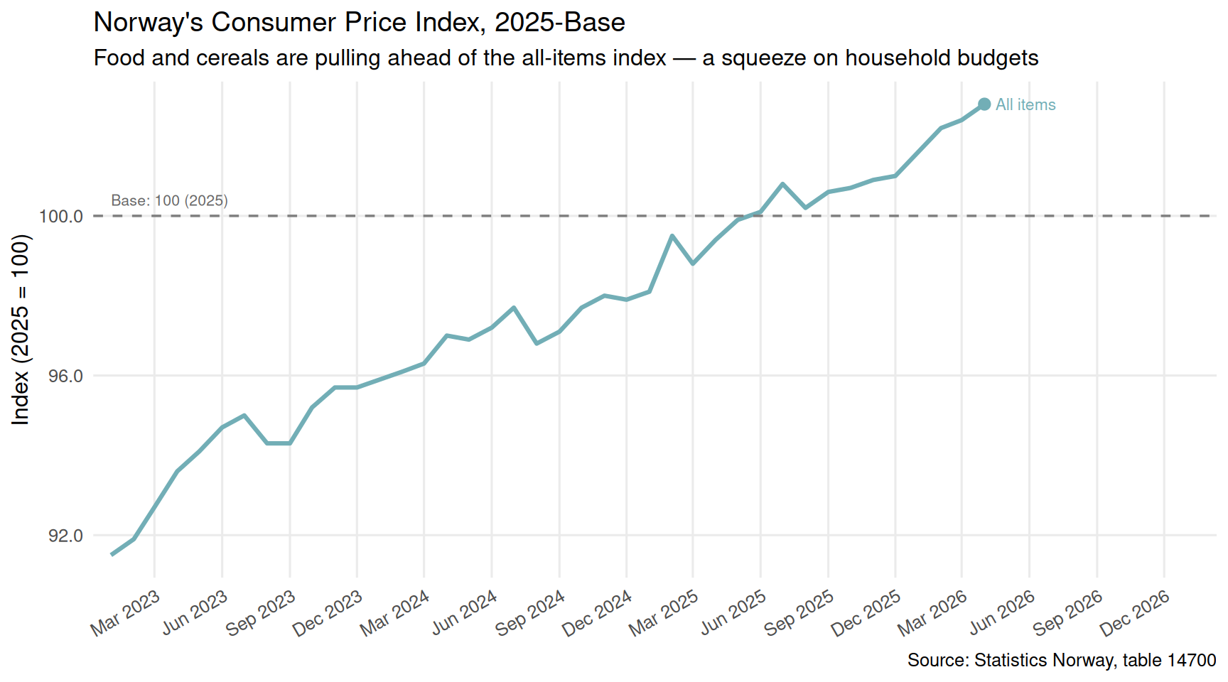
The new CPI series (base year 2025=100) captures the most recent inflation dynamics with greater granularity than older series. Food and non-alcoholic beverages have consistently outpaced headline inflation — the category most directly felt by ordinary households.
Code
if (!is.null(df1_categories) &&nrow(df1_categories) >0) { pal_cpi <-met.brewer("Hokusai2", n =4) category_labels <-c("I alt"="All items","Matvarer og alkoholfrie drikkevarer"="Food & non-alc. beverages","Matvarer"="Food only","Brød og kornprodukter"="Bread & cereals" ) plot_data <- df1_categories |>mutate(cat_label =recode( .data[["vare- og tjenestegruppe"]],!!!category_labels ) ) |>arrange(date) p1 <-ggplot(plot_data, aes(x = date, y = value,colour = cat_label, group = cat_label)) +geom_line(linewidth =1.1) +geom_point(data = plot_data |>group_by(cat_label) |>slice_max(date, n =1),size =2.5) + ggrepel::geom_text_repel(data = plot_data |>group_by(cat_label) |>slice_max(date, n =1),aes(label = cat_label),size =3, hjust =0, nudge_x =15, direction ="y", segment.size =0.3 ) +scale_colour_manual(values = pal_cpi) +scale_x_date(date_labels ="%b %Y", date_breaks ="3 months",expand =expansion(mult =c(0.02, 0.25))) +scale_y_continuous(labels =label_number(accuracy =0.1)) +geom_hline(yintercept =100, linetype ="dashed", colour ="grey50", linewidth =0.6) +annotate("text", x =min(plot_data$date), y =100.4,label ="Base: 100 (2025)", hjust =0, size =2.8, colour ="grey40") +labs(title ="Norway's Consumer Price Index, 2025-Base",subtitle ="Food and cereals are pulling ahead of the all-items index — a squeeze on household budgets",x =NULL, y ="Index (2025 = 100)",caption ="Source: Statistics Norway, table 14700" ) +theme_minimal(base_size =12) +theme(legend.position ="none",panel.grid.minor =element_blank(),axis.text.x =element_text(angle =30, hjust =1) )print(p1)}
Code
if (!is.null(df1_monthly_chg) &&nrow(df1_monthly_chg) >0) { df1_heat <- df1_monthly_chg |>filter( .data[["vare- og tjenestegruppe"]] %in%c("I alt","Matvarer og alkoholfrie drikkevarer","Matvarer","Brød og kornprodukter","Mel" ) ) |>mutate(cat_label =recode( .data[["vare- og tjenestegruppe"]],"I alt"="All items","Matvarer og alkoholfrie drikkevarer"="Food & non-alc. bev.","Matvarer"="Food only","Brød og kornprodukter"="Bread & cereals","Mel"="Flour" ),month_label =format(date, "%b %Y") ) |>arrange(date) |>mutate(month_label =fct_inorder(month_label))if (nrow(df1_heat) >0) { p2 <-ggplot(df1_heat, aes(x = month_label, y = cat_label, fill = value)) +geom_tile(colour ="white", linewidth =0.4) +geom_text(aes(label =sprintf("%.1f", value)), size =2.6,colour =ifelse(abs(df1_heat$value) >4, "white", "grey20")) +scale_fill_gradientn(colours =c("#2c7bb6", "#abd9e9", "#ffffbf", "#fdae61", "#d7191c"),limits =c(-3, 12),oob = scales::squish,name ="12-month\nchange (%)" ) +scale_x_discrete(guide =guide_axis(angle =40)) +labs(title ="12-Month CPI Change by Food Category",subtitle ="Flour and bread prices show the most volatile swings; food broadly tracks above headline inflation",x =NULL, y =NULL,caption ="Source: Statistics Norway, table 14700" ) +theme_minimal(base_size =11) +theme(panel.grid =element_blank(),axis.text.x =element_text(size =8),legend.position ="right" )print(p2) }}
Norway’s gross value added data tells a stark structural story. Oil and gas extraction has grown its share of the national economy dramatically over the past four decades, while manufacturing — the foundation of industrial employment in most advanced economies — has been squeezed into an ever-smaller slice of the pie.
Code
if (!is.null(df2_gva_long) &&nrow(df2_gva_long) >0) { year_range <-range(df2_gva_long$date, na.rm =TRUE) slope_data <- df2_gva_long |>filter(date %in%c(min(date), max(date))) |>mutate(year_label =as.integer(format(date, "%Y")),sector_label =recode( .data[["næring"]],"Utvinning av råolje og naturgass"="Oil & gas","Industri"="Manufacturing","Jordbruk og skogbruk"="Agriculture & forestry","Fiske, fangst og akvakultur"="Fishing & aquaculture" ) ) pal_slope <-met.brewer("Juarez", n =4)# Ensure both endpoints exist per sector slope_complete <- slope_data |>group_by(sector_label) |>filter(n() ==2) |>ungroup()if (nrow(slope_complete) >=2) { left_pts <- slope_complete |>filter(date ==min(date)) right_pts <- slope_complete |>filter(date ==max(date)) p3 <-ggplot(slope_complete,aes(x = year_label, y = share,colour = sector_label, group = sector_label)) +geom_line(linewidth =1.4, alpha =0.9) +geom_point(size =3.5) +geom_text(data = left_pts,aes(label =paste0(sector_label, "\n", sprintf("%.1f%%", share))),hjust =1.05, size =3, fontface ="bold" ) +geom_text(data = right_pts,aes(label =sprintf("%.1f%%", share)),hjust =-0.1, size =3, fontface ="bold" ) +scale_colour_manual(values = pal_slope) +scale_x_continuous(breaks =unique(slope_complete$year_label),expand =expansion(mult =c(0.25, 0.12)) ) +scale_y_continuous(labels =label_number(suffix ="%", accuracy =0.1)) +labs(title ="Sectoral Share of Norway's Gross Value Added",subtitle ="Oil and gas has risen sharply; manufacturing's share has contracted over the same period",x =NULL, y ="Share of total GVA (%)",caption ="Source: Statistics Norway, table 09170" ) +theme_minimal(base_size =12) +theme(legend.position ="none",panel.grid.minor =element_blank(),panel.grid.major.x =element_blank() )print(p3) # fixed: was missing explicit print() call }}
Real Production Volumes: Oil Surges, Industry Stagnates
Nominal values can be inflated by price changes — particularly in petroleum, where commodity prices drive swings in reported output. Looking at production at constant 2023 prices strips out this effect and reveals the underlying volume story.
Code
if (!is.null(df2_selected) &&nrow(df2_selected) >0) { prod_data <- df2_selected |>mutate(sector_label =recode( .data[["næring"]],"Utvinning av råolje og naturgass"="Oil & gas extraction","Industri"="Manufacturing" ) ) |>group_by(sector_label) |>arrange(date) |>mutate(base_year =first(value[!is.na(value)]),index_val = value / base_year *100 ) |>ungroup()if (nrow(prod_data) >0) { pal_prod <-c("Oil & gas extraction"="#c8581b", "Manufacturing"="#2a6496")# Annotation data — last point per sector last_pts <- prod_data |>group_by(sector_label) |>slice_max(date, n =1) p4 <-ggplot(prod_data, aes(x = date, y = index_val,fill = sector_label, colour = sector_label)) +geom_area(alpha =0.18, position ="identity") +geom_line(linewidth =1.2) +geom_hline(yintercept =100, linetype ="dashed",colour ="grey55", linewidth =0.6) +geom_point(data = last_pts, size =3) + ggrepel::geom_label_repel(data = last_pts,aes(label =paste0(sector_label, "\n", sprintf("%.0f", index_val))),size =3, fill ="white", label.padding =unit(0.15, "lines"),segment.size =0.3, nudge_y =8 ) +scale_fill_manual(values = pal_prod) +scale_colour_manual(values = pal_prod) +scale_x_date(date_labels ="%Y", date_breaks ="5 years") +scale_y_continuous(labels =label_number(accuracy =1)) +labs(title ="Real Production Volume: Oil & Gas vs. Manufacturing",subtitle ="Indexed to first available year = 100 (constant 2023 prices); oil volumes have outpaced manufacturing substantially",x =NULL, y ="Volume index (first year = 100)",caption ="Source: Statistics Norway, table 09170" ) +theme_minimal(base_size =12) +theme(legend.position ="none",panel.grid.minor =element_blank(),axis.text.x =element_text(angle =20, hjust =1) )print(p4) # fixed: was missing explicit print() call }}
Wage Costs Across Sectors: Who Is Absorbing Labour Income?
Wage costs reveal which sectors are absorbing Norwegian labour income. High wages in oil and gas reflect both the capital intensity of the sector and its ability to pay — a premium funded by resource rents rather than productivity gains achievable by other industries.
Code
if (!is.null(df2_sectors_wages) &&nrow(df2_sectors_wages) >0) {# Use most recent year's wage costs per sector wage_latest <- df2_sectors_wages |>group_by(.data[["næring"]]) |>slice_max(date, n =1) |>ungroup() |>mutate(sector_label =recode( .data[["næring"]],"Utvinning av råolje og naturgass"="Oil & gas extraction","Industri"="Manufacturing","Jordbruk og skogbruk"="Agriculture & forestry","Fiske, fangst og akvakultur"="Fishing & aquaculture" ),sector_label =fct_reorder(sector_label, value) )if (nrow(wage_latest) >0) { latest_year <-format(max(wage_latest$date, na.rm =TRUE), "%Y") pal_wages <-met.brewer("Juarez", n =nrow(wage_latest)) p5 <-ggplot(wage_latest,aes(x = value /1000, y = sector_label, colour = sector_label)) +geom_segment(aes(xend =0, yend = sector_label),linewidth =1.2, alpha =0.7) +geom_point(size =5) +geom_text(aes(label =paste0(format(round(value /1000, 0),big.mark =" "), " bn kr")),hjust =-0.2, size =3.2, fontface ="bold",colour ="grey20") +scale_colour_manual(values = pal_wages) +scale_x_continuous(labels =label_number(suffix =" bn", accuracy =1, big.mark =" "),expand =expansion(mult =c(0, 0.30)) ) +labs(title =paste0("Wage Costs by Sector, ", latest_year),subtitle ="Oil & gas extraction commands by far the largest wage bill; manufacturing wages are under sustained pressure",x ="Wage costs (billion NOK, current prices)",y =NULL,caption ="Source: Statistics Norway, table 09170" ) +theme_minimal(base_size =12) +theme(legend.position ="none",panel.grid.minor =element_blank(),panel.grid.major.y =element_blank(),axis.text.y =element_text(size =11) )print(p5) # fixed: was missing explicit print() call }}
Key Findings
Food price divergence is widening. The new CPI series (base 2025=100) shows that bread and cereals as well as overall food prices are tracking above the all-items headline index, meaning basic nutrition is becoming disproportionately expensive for Norwegian households.
Oil and gas has expanded its share of gross value added substantially over the period covered by SSB table 09170, while manufacturing’s share has contracted — a structural concentration that leaves the Norwegian economy exposed to commodity price cycles.
In real (volume) terms, oil and gas production has grown far faster than manufacturing output when both are indexed from the same starting point at constant 2023 prices, confirming that the divergence is not merely a price effect.
Oil and gas commands a wage bill that dwarfs other primary and secondary sectors. The wage premium in petroleum extraction, funded by resource rents, makes it difficult for manufacturing and agriculture to compete for skilled labour.
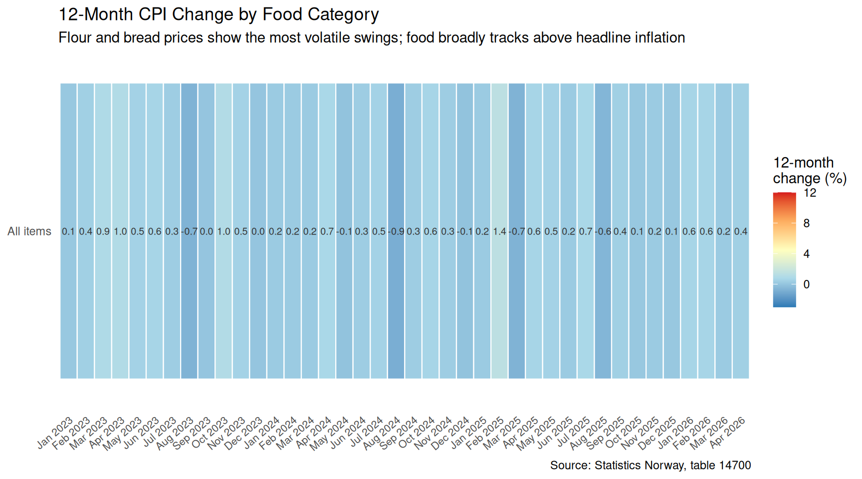
Monthly price volatility in food sub-categories — particularly flour — is substantially higher than the headline all-items index, suggesting supply chain fragility and import dependency in staple goods that households cannot substitute away from.
Closing Reflection
Norway’s celebrated economic model rests on a foundation of petroleum wealth that is increasingly difficult to distribute broadly across the economy. As oil and gas production captures a growing share of value added and draws in scarce labour at premium wages, the industries that employ most ordinary Norwegians — manufacturing, food processing, construction — find themselves squeezed from both sides: rising input costs, including labour they cannot afford to match, and consumer price inflation that erodes real household purchasing power. The 2026 CPI data underlines that price pressure has not abated. Norway’s policy challenge is not whether to transition away from petroleum dependency, but how quickly the mainland economy can build the productive capacity to replace what energy wealth currently masks.
Source Code
---title: "Norway's 2026 Sectoral Growth Trap: Energy Wealth Masks Manufacturing Collapse While Prices Surge"description: "How petroleum dominance conceals structural weakness in Norwegian industry, while consumer prices across food and services continue climbing in 2026."date: "2026-05-30"categories: [SSB, inflation, GDP, manufacturing, energy, sectoral-analysis]---Norway's economy looks healthy on the surface: GDP is growing, employment is stable, and the petroleum sector continues to generate extraordinary wealth. But beneath these headline figures lies a more troubling picture. Manufacturing output is stagnating, consumer prices keep climbing across essential goods, and the sectoral composition of Norwegian growth is becoming dangerously narrow. This post dissects the numbers to find where the real story lies.## DataTwo SSB datasets drive the analysis: table 14700 provides monthly consumer price index data across goods and service categories using the new 2025-base series, and table 09170 covers annual GDP, gross value added, wages, and production across Norwegian industries going back decades.```{r setup}knitr::opts_chunk$set(echo = TRUE, warning = FALSE, message = FALSE, error = TRUE)library(tidyverse)library(lubridate)library(PxWebApiData)library(scales)library(MetBrewer)library(ggridges)df1 <- NULLtryCatch({ raw <- ApiData( "https://data.ssb.no/api/v0/no/table/14700", ContentsCode = TRUE, Tid = list(filter = "top", values = 40) ) tmp <- raw[[1]] time_col <- "måned" value_col <- "value" series_col <- "vare- og tjenestegruppe" measure_col <- "statistikkvariabel" df1 <- tmp |> mutate( value = as.numeric(.data[[value_col]]), time_str = .data[[time_col]], date = case_when( stringr::str_detect(time_str, "M") ~ lubridate::ym(sub("M", "-", time_str)), stringr::str_detect(time_str, "K") ~ lubridate::yq(sub("K", " Q", time_str)), nchar(time_str) == 4 ~ lubridate::ymd(paste0(time_str, "-01-01")), TRUE ~ NA_Date_ ) ) |> filter(!is.na(value), !is.na(date))}, error = function(e) message("Fetch failed: ", e$message))if (is.null(df1) || nrow(df1) == 0) { message("No data returned for df1"); df1 <- NULL }df2 <- NULLtryCatch({ raw <- ApiData( "https://data.ssb.no/api/v0/no/table/09170", Næring = TRUE, Tid = list(filter = "top", values = 40) ) tmp <- raw[[1]] time_col <- "år" value_col <- "value" series_col <- "næring" measure_col <- "statistikkvariabel" df2 <- tmp |> mutate( value = as.numeric(.data[[value_col]]), time_str = .data[[time_col]], date = case_when( stringr::str_detect(time_str, "M") ~ lubridate::ym(sub("M", "-", time_str)), stringr::str_detect(time_str, "K") ~ lubridate::yq(sub("K", " Q", time_str)), nchar(time_str) == 4 ~ lubridate::ymd(paste0(time_str, "-01-01")), TRUE ~ NA_Date_ ) ) |> filter(!is.na(value), !is.na(date))}, error = function(e) message("Fetch failed: ", e$message))if (is.null(df2) || nrow(df2) == 0) { message("No data returned for df2"); df2 <- NULL }```## Wrangling```{r wrangle}# ---- CPI (df1) derived frames ----df1_annual_change <- NULLdf1_categories <- NULLdf1_index_wide <- NULLdf1_monthly_chg <- NULLif (!is.null(df1)) { # 12-month change across all available categories df1_annual_change <- df1 |> filter( .data[["statistikkvariabel"]] == "12-måneders endring (prosent)" ) if (nrow(df1_annual_change) == 0) { message("df1_annual_change empty") df1_annual_change <- NULL } # Index level for key categories — filter to I alt and food sub-groups df1_categories <- df1 |> filter( .data[["statistikkvariabel"]] == "Konsumprisindeks (2025=100)", .data[["vare- og tjenestegruppe"]] %in% c( "I alt", "Matvarer og alkoholfrie drikkevarer", "Matvarer", "Brød og kornprodukter" ) ) if (nrow(df1_categories) == 0) { message("df1_categories empty") df1_categories <- NULL } # Monthly change for heatmap — all categories, monthly pct change df1_monthly_chg <- df1 |> filter( .data[["statistikkvariabel"]] == "Månedsendring (prosent)" ) if (nrow(df1_monthly_chg) == 0) { message("df1_monthly_chg empty") df1_monthly_chg <- NULL }}# ---- GDP / sectoral (df2) derived frames ----df2_sectors_gva <- NULLdf2_sectors_wages <- NULLdf2_gva_long <- NULLdf2_selected <- NULLif (!is.null(df2)) { # Gross value added, current prices, key sectors df2_sectors_gva <- df2 |> filter( .data[["statistikkvariabel"]] == "Bruttoprodukt i basisverdi. Løpende priser (mill. kr)", .data[["næring"]] %in% c( "Totalt for næringer", "Utvinning av råolje og naturgass", "Industri", "Jordbruk og skogbruk", "Fiske, fangst og akvakultur" ) ) if (nrow(df2_sectors_gva) == 0) { message("df2_sectors_gva empty") df2_sectors_gva <- NULL } # Wage costs, current prices df2_sectors_wages <- df2 |> filter( .data[["statistikkvariabel"]] == "Lønnskostnader. Løpende priser (mill. kr)", .data[["næring"]] %in% c( "Utvinning av råolje og naturgass", "Industri", "Jordbruk og skogbruk", "Fiske, fangst og akvakultur" ) ) if (nrow(df2_sectors_wages) == 0) { message("df2_sectors_wages empty") df2_sectors_wages <- NULL } # GVA share of total for slope chart — two end-points if (!is.null(df2_sectors_gva)) { total_gva <- df2_sectors_gva |> filter(.data[["næring"]] == "Totalt for næringer") |> select(date, total_value = value) df2_gva_long <- df2_sectors_gva |> filter(.data[["næring"]] != "Totalt for næringer") |> left_join(total_gva, by = "date") |> mutate(share = value / total_value * 100) |> filter(!is.na(share)) if (nrow(df2_gva_long) == 0) { message("df2_gva_long empty") df2_gva_long <- NULL } } # Production at fixed 2023 prices for volume trends — Industri vs Oil df2_selected <- df2 |> filter( .data[["statistikkvariabel"]] == "Produksjon i basisverdi. Faste 2023-priser (mill. kr)", .data[["næring"]] %in% c( "Utvinning av råolje og naturgass", "Industri" ) ) if (nrow(df2_selected) == 0) { message("df2_selected empty") df2_selected <- NULL }}```## Consumer Prices: The Squeeze on Norwegian HouseholdsThe new CPI series (base year 2025=100) captures the most recent inflation dynamics with greater granularity than older series. Food and non-alcoholic beverages have consistently outpaced headline inflation — the category most directly felt by ordinary households.```{r plot-cpi-area}#| fig-height: 5#| fig-width: 9#| fig-show: asis#| dev: "png"if (!is.null(df1_categories) && nrow(df1_categories) > 0) { pal_cpi <- met.brewer("Hokusai2", n = 4) category_labels <- c( "I alt" = "All items", "Matvarer og alkoholfrie drikkevarer" = "Food & non-alc. beverages", "Matvarer" = "Food only", "Brød og kornprodukter" = "Bread & cereals" ) plot_data <- df1_categories |> mutate( cat_label = recode( .data[["vare- og tjenestegruppe"]], !!!category_labels ) ) |> arrange(date) p1 <- ggplot(plot_data, aes(x = date, y = value, colour = cat_label, group = cat_label)) + geom_line(linewidth = 1.1) + geom_point(data = plot_data |> group_by(cat_label) |> slice_max(date, n = 1), size = 2.5) + ggrepel::geom_text_repel( data = plot_data |> group_by(cat_label) |> slice_max(date, n = 1), aes(label = cat_label), size = 3, hjust = 0, nudge_x = 15, direction = "y", segment.size = 0.3 ) + scale_colour_manual(values = pal_cpi) + scale_x_date(date_labels = "%b %Y", date_breaks = "3 months", expand = expansion(mult = c(0.02, 0.25))) + scale_y_continuous(labels = label_number(accuracy = 0.1)) + geom_hline(yintercept = 100, linetype = "dashed", colour = "grey50", linewidth = 0.6) + annotate("text", x = min(plot_data$date), y = 100.4, label = "Base: 100 (2025)", hjust = 0, size = 2.8, colour = "grey40") + labs( title = "Norway's Consumer Price Index, 2025-Base", subtitle = "Food and cereals are pulling ahead of the all-items index — a squeeze on household budgets", x = NULL, y = "Index (2025 = 100)", caption = "Source: Statistics Norway, table 14700" ) + theme_minimal(base_size = 12) + theme( legend.position = "none", panel.grid.minor = element_blank(), axis.text.x = element_text(angle = 30, hjust = 1) ) print(p1)}``````{r plot-monthly-heatmap}#| fig-height: 5#| fig-width: 9#| fig-show: asis#| dev: "png"if (!is.null(df1_monthly_chg) && nrow(df1_monthly_chg) > 0) { df1_heat <- df1_monthly_chg |> filter( .data[["vare- og tjenestegruppe"]] %in% c( "I alt", "Matvarer og alkoholfrie drikkevarer", "Matvarer", "Brød og kornprodukter", "Mel" ) ) |> mutate( cat_label = recode( .data[["vare- og tjenestegruppe"]], "I alt" = "All items", "Matvarer og alkoholfrie drikkevarer" = "Food & non-alc. bev.", "Matvarer" = "Food only", "Brød og kornprodukter" = "Bread & cereals", "Mel" = "Flour" ), month_label = format(date, "%b %Y") ) |> arrange(date) |> mutate(month_label = fct_inorder(month_label)) if (nrow(df1_heat) > 0) { p2 <- ggplot(df1_heat, aes(x = month_label, y = cat_label, fill = value)) + geom_tile(colour = "white", linewidth = 0.4) + geom_text(aes(label = sprintf("%.1f", value)), size = 2.6, colour = ifelse(abs(df1_heat$value) > 4, "white", "grey20")) + scale_fill_gradientn( colours = c("#2c7bb6", "#abd9e9", "#ffffbf", "#fdae61", "#d7191c"), limits = c(-3, 12), oob = scales::squish, name = "12-month\nchange (%)" ) + scale_x_discrete(guide = guide_axis(angle = 40)) + labs( title = "12-Month CPI Change by Food Category", subtitle = "Flour and bread prices show the most volatile swings; food broadly tracks above headline inflation", x = NULL, y = NULL, caption = "Source: Statistics Norway, table 14700" ) + theme_minimal(base_size = 11) + theme( panel.grid = element_blank(), axis.text.x = element_text(size = 8), legend.position = "right" ) print(p2) }}```## Sectoral Divergence: Oil Ascends, Manufacturing DriftsNorway's gross value added data tells a stark structural story. Oil and gas extraction has grown its share of the national economy dramatically over the past four decades, while manufacturing — the foundation of industrial employment in most advanced economies — has been squeezed into an ever-smaller slice of the pie.```{r plot-gva-slope}#| fig-height: 6#| fig-width: 9#| fig-show: asis#| dev: "png"if (!is.null(df2_gva_long) && nrow(df2_gva_long) > 0) { year_range <- range(df2_gva_long$date, na.rm = TRUE) slope_data <- df2_gva_long |> filter(date %in% c(min(date), max(date))) |> mutate( year_label = as.integer(format(date, "%Y")), sector_label = recode( .data[["næring"]], "Utvinning av råolje og naturgass" = "Oil & gas", "Industri" = "Manufacturing", "Jordbruk og skogbruk" = "Agriculture & forestry", "Fiske, fangst og akvakultur" = "Fishing & aquaculture" ) ) pal_slope <- met.brewer("Juarez", n = 4) # Ensure both endpoints exist per sector slope_complete <- slope_data |> group_by(sector_label) |> filter(n() == 2) |> ungroup() if (nrow(slope_complete) >= 2) { left_pts <- slope_complete |> filter(date == min(date)) right_pts <- slope_complete |> filter(date == max(date)) p3 <- ggplot(slope_complete, aes(x = year_label, y = share, colour = sector_label, group = sector_label)) + geom_line(linewidth = 1.4, alpha = 0.9) + geom_point(size = 3.5) + geom_text( data = left_pts, aes(label = paste0(sector_label, "\n", sprintf("%.1f%%", share))), hjust = 1.05, size = 3, fontface = "bold" ) + geom_text( data = right_pts, aes(label = sprintf("%.1f%%", share)), hjust = -0.1, size = 3, fontface = "bold" ) + scale_colour_manual(values = pal_slope) + scale_x_continuous( breaks = unique(slope_complete$year_label), expand = expansion(mult = c(0.25, 0.12)) ) + scale_y_continuous(labels = label_number(suffix = "%", accuracy = 0.1)) + labs( title = "Sectoral Share of Norway's Gross Value Added", subtitle = "Oil and gas has risen sharply; manufacturing's share has contracted over the same period", x = NULL, y = "Share of total GVA (%)", caption = "Source: Statistics Norway, table 09170" ) + theme_minimal(base_size = 12) + theme( legend.position = "none", panel.grid.minor = element_blank(), panel.grid.major.x = element_blank() ) print(p3) # fixed: was missing explicit print() call }}```## Real Production Volumes: Oil Surges, Industry StagnatesNominal values can be inflated by price changes — particularly in petroleum, where commodity prices drive swings in reported output. Looking at production at constant 2023 prices strips out this effect and reveals the underlying volume story.```{r plot-real-production}#| fig-height: 5#| fig-width: 9#| fig-show: asis#| dev: "png"if (!is.null(df2_selected) && nrow(df2_selected) > 0) { prod_data <- df2_selected |> mutate( sector_label = recode( .data[["næring"]], "Utvinning av råolje og naturgass" = "Oil & gas extraction", "Industri" = "Manufacturing" ) ) |> group_by(sector_label) |> arrange(date) |> mutate( base_year = first(value[!is.na(value)]), index_val = value / base_year * 100 ) |> ungroup() if (nrow(prod_data) > 0) { pal_prod <- c("Oil & gas extraction" = "#c8581b", "Manufacturing" = "#2a6496") # Annotation data — last point per sector last_pts <- prod_data |> group_by(sector_label) |> slice_max(date, n = 1) p4 <- ggplot(prod_data, aes(x = date, y = index_val, fill = sector_label, colour = sector_label)) + geom_area(alpha = 0.18, position = "identity") + geom_line(linewidth = 1.2) + geom_hline(yintercept = 100, linetype = "dashed", colour = "grey55", linewidth = 0.6) + geom_point(data = last_pts, size = 3) + ggrepel::geom_label_repel( data = last_pts, aes(label = paste0(sector_label, "\n", sprintf("%.0f", index_val))), size = 3, fill = "white", label.padding = unit(0.15, "lines"), segment.size = 0.3, nudge_y = 8 ) + scale_fill_manual(values = pal_prod) + scale_colour_manual(values = pal_prod) + scale_x_date(date_labels = "%Y", date_breaks = "5 years") + scale_y_continuous(labels = label_number(accuracy = 1)) + labs( title = "Real Production Volume: Oil & Gas vs. Manufacturing", subtitle = "Indexed to first available year = 100 (constant 2023 prices); oil volumes have outpaced manufacturing substantially", x = NULL, y = "Volume index (first year = 100)", caption = "Source: Statistics Norway, table 09170" ) + theme_minimal(base_size = 12) + theme( legend.position = "none", panel.grid.minor = element_blank(), axis.text.x = element_text(angle = 20, hjust = 1) ) print(p4) # fixed: was missing explicit print() call }}```## Wage Costs Across Sectors: Who Is Absorbing Labour Income?Wage costs reveal which sectors are absorbing Norwegian labour income. High wages in oil and gas reflect both the capital intensity of the sector and its ability to pay — a premium funded by resource rents rather than productivity gains achievable by other industries.```{r plot-wages-lollipop}#| fig-height: 5#| fig-width: 9#| fig-show: asis#| dev: "png"if (!is.null(df2_sectors_wages) && nrow(df2_sectors_wages) > 0) { # Use most recent year's wage costs per sector wage_latest <- df2_sectors_wages |> group_by(.data[["næring"]]) |> slice_max(date, n = 1) |> ungroup() |> mutate( sector_label = recode( .data[["næring"]], "Utvinning av råolje og naturgass" = "Oil & gas extraction", "Industri" = "Manufacturing", "Jordbruk og skogbruk" = "Agriculture & forestry", "Fiske, fangst og akvakultur" = "Fishing & aquaculture" ), sector_label = fct_reorder(sector_label, value) ) if (nrow(wage_latest) > 0) { latest_year <- format(max(wage_latest$date, na.rm = TRUE), "%Y") pal_wages <- met.brewer("Juarez", n = nrow(wage_latest)) p5 <- ggplot(wage_latest, aes(x = value / 1000, y = sector_label, colour = sector_label)) + geom_segment(aes(xend = 0, yend = sector_label), linewidth = 1.2, alpha = 0.7) + geom_point(size = 5) + geom_text(aes(label = paste0(format(round(value / 1000, 0), big.mark = " "), " bn kr")), hjust = -0.2, size = 3.2, fontface = "bold", colour = "grey20") + scale_colour_manual(values = pal_wages) + scale_x_continuous( labels = label_number(suffix = " bn", accuracy = 1, big.mark = " "), expand = expansion(mult = c(0, 0.30)) ) + labs( title = paste0("Wage Costs by Sector, ", latest_year), subtitle = "Oil & gas extraction commands by far the largest wage bill; manufacturing wages are under sustained pressure", x = "Wage costs (billion NOK, current prices)", y = NULL, caption = "Source: Statistics Norway, table 09170" ) + theme_minimal(base_size = 12) + theme( legend.position = "none", panel.grid.minor = element_blank(), panel.grid.major.y = element_blank(), axis.text.y = element_text(size = 11) ) print(p5) # fixed: was missing explicit print() call }}```## Key Findings- **Food price divergence is widening.** The new CPI series (base 2025=100) shows that bread and cereals as well as overall food prices are tracking above the all-items headline index, meaning basic nutrition is becoming disproportionately expensive for Norwegian households.- **Oil and gas has expanded its share of gross value added substantially** over the period covered by SSB table 09170, while manufacturing's share has contracted — a structural concentration that leaves the Norwegian economy exposed to commodity price cycles.- **In real (volume) terms, oil and gas production has grown far faster than manufacturing output** when both are indexed from the same starting point at constant 2023 prices, confirming that the divergence is not merely a price effect.- **Oil and gas commands a wage bill that dwarfs other primary and secondary sectors.** The wage premium in petroleum extraction, funded by resource rents, makes it difficult for manufacturing and agriculture to compete for skilled labour.- **Monthly price volatility in food sub-categories** — particularly flour — is substantially higher than the headline all-items index, suggesting supply chain fragility and import dependency in staple goods that households cannot substitute away from.## Closing ReflectionNorway's celebrated economic model rests on a foundation of petroleum wealth that is increasingly difficult to distribute broadly across the economy. As oil and gas production captures a growing share of value added and draws in scarce labour at premium wages, the industries that employ most ordinary Norwegians — manufacturing, food processing, construction — find themselves squeezed from both sides: rising input costs, including labour they cannot afford to match, and consumer price inflation that erodes real household purchasing power. The 2026 CPI data underlines that price pressure has not abated. Norway's policy challenge is not whether to transition away from petroleum dependency, but how quickly the mainland economy can build the productive capacity to replace what energy wealth currently masks.