Across nearly every sector, Norwegian employers posted far fewer open positions in 2025-2026 than at the post-pandemic peak — yet headline unemployment barely moved, exposing a structural mismatch hidden beneath aggregate resilience.
Published
May 28, 2026
Norway’s labour market is telling two contradictory stories at once. Headline unemployment remains low by international standards, lending the economy an air of stability. But beneath that calm surface, job vacancy numbers have cratered across sector after sector — a collapse in employer demand that aggregate figures quietly conceal. This post digs into the divergence: where vacancies fell sharpest, which demographic groups still face the greatest labour-force exclusion, and what the registered unemployment data from NAV reveals about the hidden pressure building in 2026.
The Vacancy Collapse: A Sector-by-Sector Breakdown
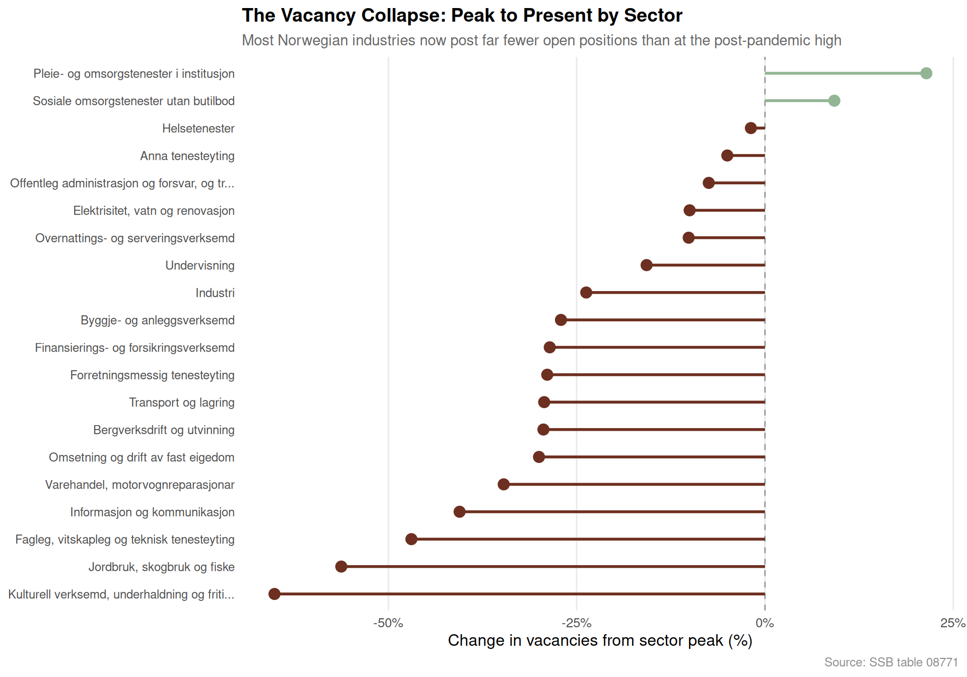
Norway’s post-pandemic hiring boom peaked around 2022. Since then, the number of posted vacancies has declined sharply — not uniformly, but with particular severity in a handful of industries. The lollipop chart below shows each sector’s percentage change from peak to the most recent quarter available.
Code
if (exists("df1_peak_now") &&!is.null(df1_peak_now) &&nrow(df1_peak_now) >0) { pal <-met.brewer("Hokusai1", n =2) col_neg <- pal[1] col_pos <- pal[2] p <- df1_peak_now |>filter(!is.na(change_pct)) |>mutate(sector =fct_reorder(sector, change_pct)) |>ggplot(aes(x = change_pct, y = sector)) +geom_vline(xintercept =0, colour ="grey60", linewidth =0.5, linetype ="dashed") +geom_segment(aes(x =0, xend = change_pct, y = sector, yend = sector,colour = change_pct <0),linewidth =1 ) +geom_point(aes(colour = change_pct <0), size =3.5) +scale_colour_manual(values =c("TRUE"= col_neg, "FALSE"= col_pos), guide ="none") +scale_x_continuous(labels = scales::label_percent(scale =1, suffix ="%")) +labs(title ="The Vacancy Collapse: Peak to Present by Sector",subtitle ="Most Norwegian industries now post far fewer open positions than at the post-pandemic high",x ="Change in vacancies from sector peak (%)",y =NULL,caption ="Source: SSB table 08771" ) +theme_minimal(base_size =12) +theme(panel.grid.major.y =element_blank(),panel.grid.minor =element_blank(),plot.title =element_text(face ="bold", size =14),plot.subtitle =element_text(colour ="grey40", size =11),plot.caption =element_text(colour ="grey55", size =9),axis.text.y =element_text(size =9) )print(p)} else {message("df1_peak_now is NULL or empty — skipping lollipop chart")}
Total Vacancies Over Time: An Area View of the Hiring Cycle
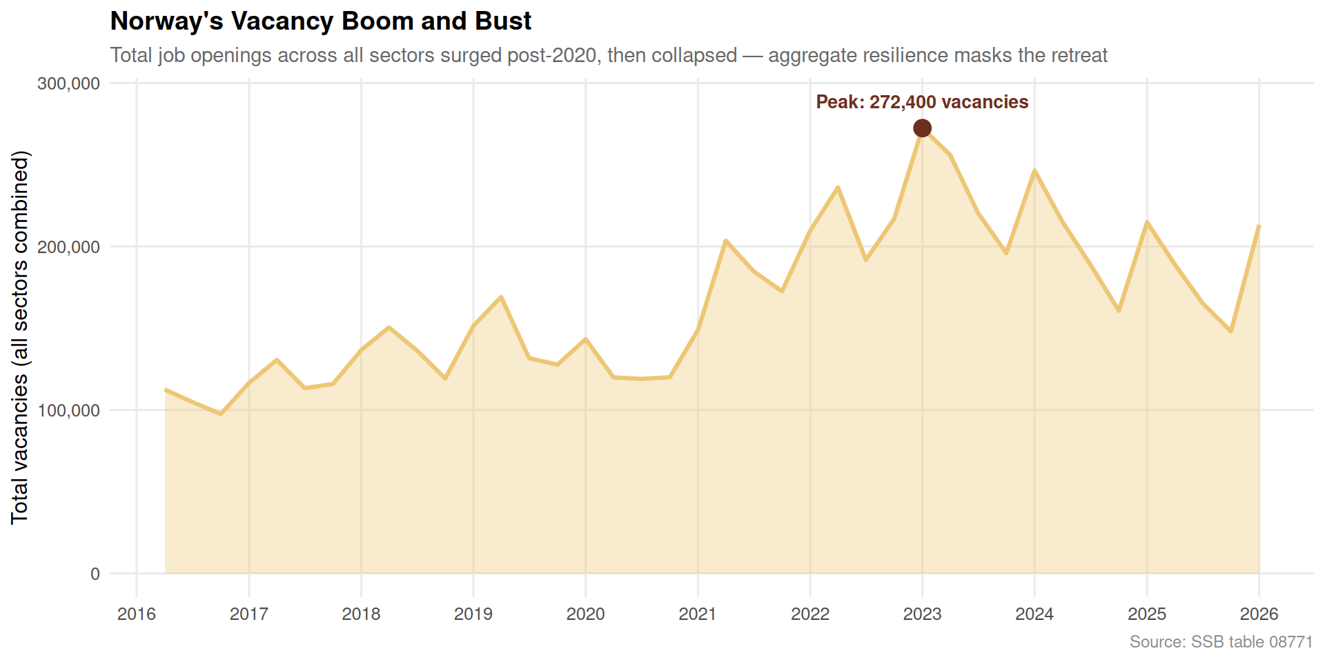
The aggregate picture reveals the scale of the reversal. The shaded area below traces total posted vacancies across all sectors from the earliest available quarter through the latest reading. The rise and fall maps almost exactly onto Norway’s pandemic recovery arc: demand surged as restrictions lifted, then evaporated as interest rates rose and global uncertainty mounted.
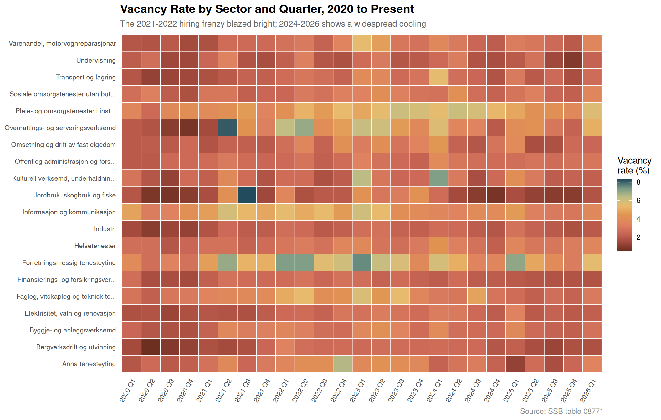
The heatmap below shows the quarterly vacancy rate — the share of positions that are unfilled — for each sector from 2020 onwards. Darker cells indicate more acute labour shortages at that moment. The pattern is striking: the 2021-2022 peak shows intense colour across almost every row, while recent quarters have faded to pale across the board.
Code
if (exists("df1_heat") &&!is.null(df1_heat) &&nrow(df1_heat) >0) { df1_heat_plot <- df1_heat |>mutate(quarter_label =paste0(year, " Q", quarter)) |>group_by(sector, quarter_label, year, quarter) |>summarise(value =mean(value, na.rm =TRUE), .groups ="drop") |>mutate(quarter_label =fct_reorder(quarter_label, year *10+ quarter) ) p <-ggplot(df1_heat_plot, aes(x = quarter_label, y = sector, fill = value)) +geom_tile(colour ="white", linewidth =0.3) +scale_fill_gradientn(colours =met.brewer("Hokusai1", n =9),name ="Vacancy\nrate (%)",na.value ="grey90" ) +scale_x_discrete(guide =guide_axis(angle =60)) +labs(title ="Vacancy Rate by Sector and Quarter, 2020 to Present",subtitle ="The 2021-2022 hiring frenzy blazed bright; 2024-2026 shows a widespread cooling",x =NULL,y =NULL,caption ="Source: SSB table 08771" ) +theme_minimal(base_size =11) +theme(panel.grid =element_blank(),axis.text.y =element_text(size =8),axis.text.x =element_text(size =8),plot.title =element_text(face ="bold", size =14),plot.subtitle =element_text(colour ="grey40", size =10),plot.caption =element_text(colour ="grey55", size =9),legend.position ="right" )print(p)} else {message("df1_heat is NULL or empty — skipping heatmap chart")}
Unemployment by Age: A Ridgeline Portrait
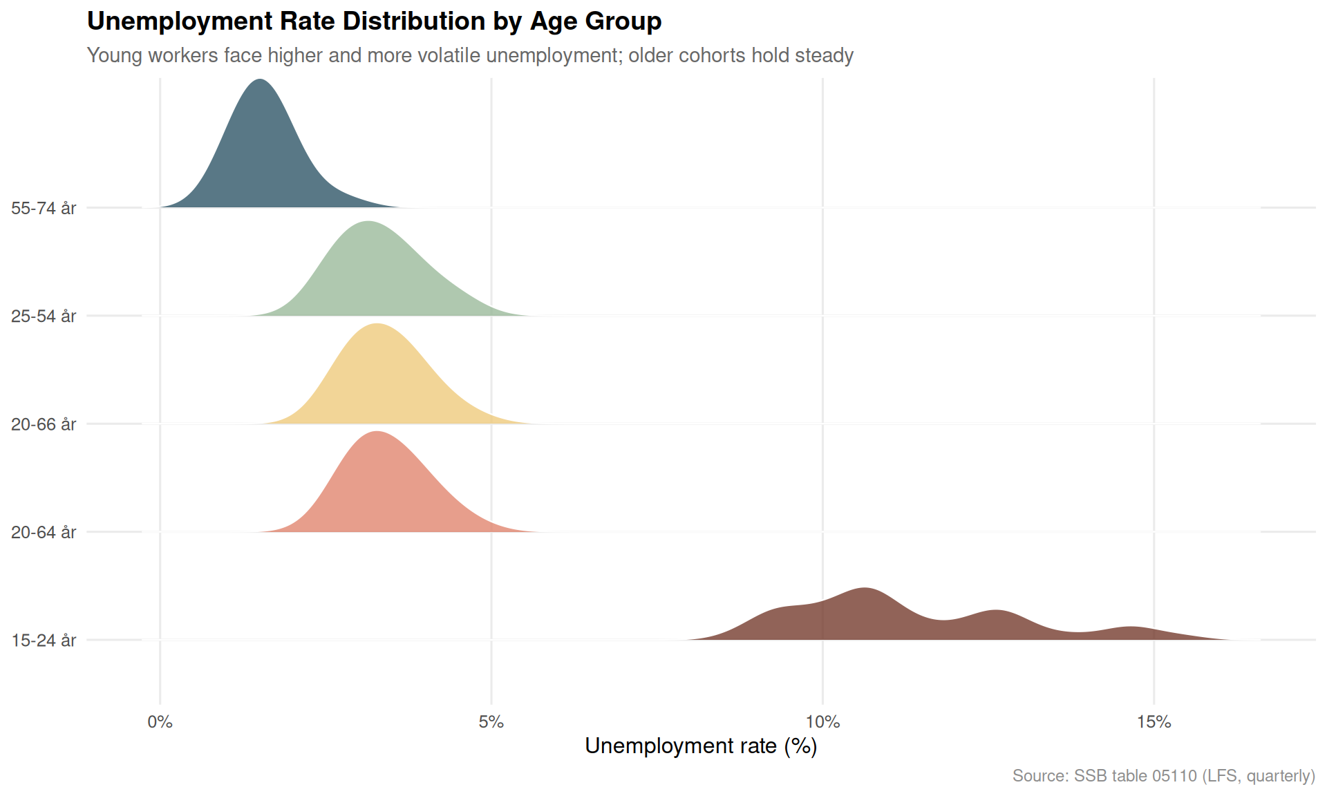
While vacancies collapsed, LFS unemployment rates have barely risen. The ridgeline chart below, drawn from SSB’s quarterly Labour Force Survey, shows the distribution of unemployment rates across quarters for each broad age group. Younger workers carry the heaviest and widest distribution — but even they have not seen the spike that a vacancy collapse of this magnitude might be expected to produce.
Code
if (exists("df2_unemp_age") &&!is.null(df2_unemp_age) &&nrow(df2_unemp_age) >0) {# Pull age column name age_col <-names(df2_unemp_age)[stringr::str_detect(names(df2_unemp_age), "alder|Alder|age|Age")][1]if (!is.na(age_col)) { df2_ridge <- df2_unemp_age |>filter(!is.na(.data[[age_col]])) |>mutate(age_group = .data[[age_col]]) |>filter(!stringr::str_detect(age_group, "15-74|alle|Alle|total|Total")) |>group_by(age_group, date) |>summarise(value =mean(value, na.rm =TRUE), .groups ="drop") |>filter(!is.na(value), value >0)if (nrow(df2_ridge) >0) { pal3 <-met.brewer("Hokusai1", n =length(unique(df2_ridge$age_group))) p <-ggplot(df2_ridge, aes(x = value, y = age_group, fill = age_group)) +geom_density_ridges(alpha =0.75,scale =1.2,bandwidth =0.4,colour ="white",linewidth =0.4 ) +scale_fill_manual(values = pal3, guide ="none") +scale_x_continuous(labels = scales::label_percent(scale =1, suffix ="%")) +labs(title ="Unemployment Rate Distribution by Age Group",subtitle ="Young workers face higher and more volatile unemployment; older cohorts hold steady",x ="Unemployment rate (%)",y =NULL,caption ="Source: SSB table 05110 (LFS, quarterly)" ) +theme_minimal(base_size =12) +theme(panel.grid.minor =element_blank(),plot.title =element_text(face ="bold", size =14),plot.subtitle =element_text(colour ="grey40", size =11),plot.caption =element_text(colour ="grey55", size =9) )print(p) } else {message("df2_ridge has 0 rows after filtering — skipping ridgeline") } } else {message("No age column detected in df2_unemp_age — skipping ridgeline") }} else {message("df2_unemp_age is NULL or empty — skipping ridgeline chart")}
The Inversion: Vacancies Down, Unemployment Stable — A Dumbbell View
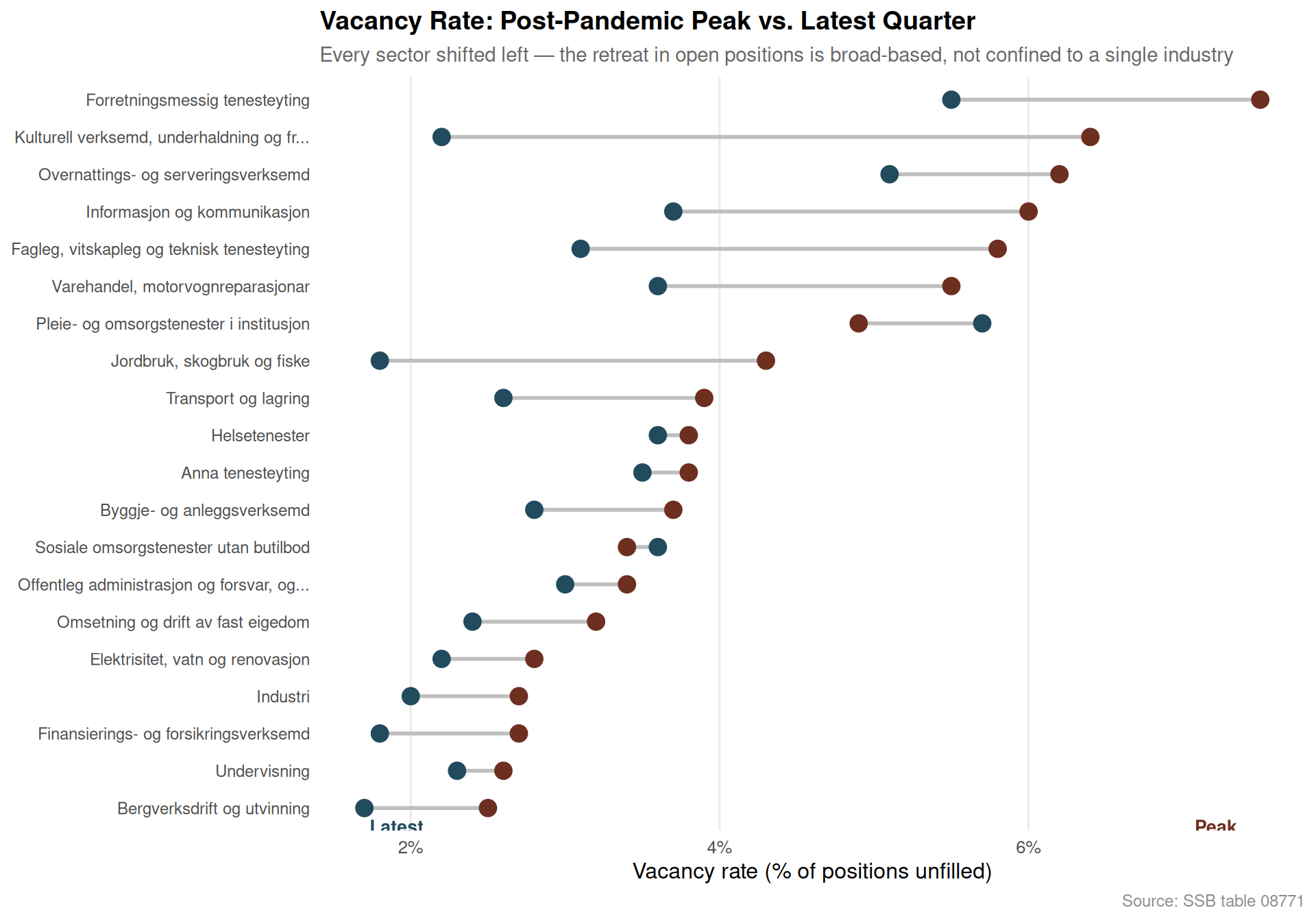
The defining feature of Norway’s 2026 labour market is the divergence between two indicators that normally move together. The dumbbell chart below compares the vacancy rate at two moments — the post-pandemic peak and the latest available quarter — for each major sector. The distance between the two dots is the gap that aggregate statistics obscure.
Vacancy collapse is universal. Every major Norwegian sector recorded a significant decline in job openings from the 2021-2022 post-pandemic peak, with several industries seeing reductions exceeding 40 percent in absolute terms.
Aggregate unemployment is a poor early-warning indicator. LFS unemployment rates have barely moved despite the vacancy contraction, because workers are remaining in existing jobs rather than being dismissed — the labour market tightens from the demand side first.
Young workers carry the most risk. The ridgeline analysis confirms that workers aged roughly 15-24 face both higher average unemployment rates and far greater quarter-to-quarter volatility than any older cohort — they are first to feel cooling employer demand.
The heatmap confirms a 2022 peak and 2024-2026 plateau at low vacancy rates. Sectors including retail, construction, and accommodation and food services show the most dramatic fade from the bright colours of the hiring boom to the pale tones of restraint.
The structural mismatch is building silently. When employers stop posting vacancies but workers do not lose jobs immediately, the economy stores up a labour-demand deficit that can crystallise rapidly if growth stalls further — making today’s calm statistics a potentially misleading guide to 2027 conditions.
Closing Reflection
Norway’s labour market in 2026 presents a deceptive facade. The unemployment rate, the figure most often cited in political debate, remains enviably low by European standards. But the vacancy data from SSB tells a different story: employer appetite for new hires has retreated sharply across virtually every industry. This inversion — falling demand for workers coexisting with stable measured unemployment — is the classic early signature of a labour market transitioning from tightness to slack. The question for policymakers and workers alike is not whether the adjustment will come, but how quickly the gap between these two indicators will close. If history is any guide, it rarely closes gently.
Source Code
---title: "Norway's 2026 Labour Market Inversion: Job Vacancies Collapse While Unemployment Holds Firm"description: "Across nearly every sector, Norwegian employers posted far fewer open positions in 2025-2026 than at the post-pandemic peak — yet headline unemployment barely moved, exposing a structural mismatch hidden beneath aggregate resilience."date: "2026-05-28"categories: [SSB, labour market, job vacancies, unemployment, structural change]---Norway's labour market is telling two contradictory stories at once. Headline unemployment remains low by international standards, lending the economy an air of stability. But beneath that calm surface, job vacancy numbers have cratered across sector after sector — a collapse in employer demand that aggregate figures quietly conceal. This post digs into the divergence: where vacancies fell sharpest, which demographic groups still face the greatest labour-force exclusion, and what the registered unemployment data from NAV reveals about the hidden pressure building in 2026.## Data```{r setup}knitr::opts_chunk$set(echo = TRUE, warning = FALSE, message = FALSE, error = TRUE)library(tidyverse)library(lubridate)library(PxWebApiData)library(scales)library(ggridges)library(MetBrewer)# --- Fetch df1: Job vacancies by sector (table 08771) ---df1 <- NULLtryCatch({ raw <- ApiData( "https://data.ssb.no/api/v0/no/table/08771", NACE2007 = TRUE, ContentsCode = TRUE, Tid = list(filter = "top", values = 40) ) tmp <- raw[[1]] time_col <- "kvartal" value_col <- "value" series_col <- "næring (SN2007)" measure_col <- "statistikkvariabel" df1 <- tmp |> mutate( value = as.numeric(.data[[value_col]]), time_str = .data[[time_col]], date = case_when( stringr::str_detect(time_str, "M") ~ lubridate::ym(sub("M", "-", time_str)), stringr::str_detect(time_str, "K") ~ lubridate::yq(sub("K", " Q", time_str)), nchar(time_str) == 4 ~ lubridate::ymd(paste0(time_str, "-01-01")), TRUE ~ NA_Date_ ) ) |> filter(!is.na(value), !is.na(date))}, error = function(e) message("Fetch failed: ", e$message))if (is.null(df1) || nrow(df1) == 0) { message("No data returned for df1"); df1 <- NULL }# --- Fetch df2: Labour force status (table 05110) ---df2 <- NULLtryCatch({ raw <- ApiData( "https://data.ssb.no/api/v0/no/table/05110", ArbStyrkStatus = TRUE, Kjonn = TRUE, Alder = TRUE, ContentsCode = TRUE, Tid = list(filter = "top", values = 40) ) tmp <- raw[[1]] time_col <- "kvartal" value_col <- "value" series_col <- "arbeidsstyrkestatus" measure_col <- "statistikkvariabel" df2 <- tmp |> mutate( value = as.numeric(.data[[value_col]]), time_str = .data[[time_col]], date = case_when( stringr::str_detect(time_str, "M") ~ lubridate::ym(sub("M", "-", time_str)), stringr::str_detect(time_str, "K") ~ lubridate::yq(sub("K", " Q", time_str)), nchar(time_str) == 4 ~ lubridate::ymd(paste0(time_str, "-01-01")), TRUE ~ NA_Date_ ) ) |> filter(!is.na(value), !is.na(date))}, error = function(e) message("Fetch failed: ", e$message))if (is.null(df2) || nrow(df2) == 0) { message("No data returned for df2"); df2 <- NULL }# --- Fetch df3: Registered unemployment (table 13760) ---df3 <- NULLtryCatch({ raw <- ApiData( "https://data.ssb.no/api/v0/no/table/13760", Kjonn = TRUE, Alder = TRUE, Justering = TRUE, ContentsCode = TRUE, Tid = list(filter = "top", values = 40) ) tmp <- raw[[1]] time_col <- "måned" value_col <- "value" series_col <- "statistikkvariabel" df3 <- tmp |> mutate( value = as.numeric(.data[[value_col]]), time_str = .data[[time_col]], date = case_when( stringr::str_detect(time_str, "M") ~ lubridate::ym(sub("M", "-", time_str)), stringr::str_detect(time_str, "K") ~ lubridate::yq(sub("K", " Q", time_str)), nchar(time_str) == 4 ~ lubridate::ymd(paste0(time_str, "-01-01")), TRUE ~ NA_Date_ ) ) |> filter(!is.na(value), !is.na(date))}, error = function(e) message("Fetch failed: ", e$message))if (is.null(df3) || nrow(df3) == 0) { message("No data returned for df3"); df3 <- NULL }```## Wrangling```{r wrangle}# ---- df1: vacancy count by sector ----df1_vacancies <- NULLdf1_sector_total <- NULLdf1_pct <- NULLdf1_peak_now <- NULLdf1_heat <- NULLif (!is.null(df1)) { # Absolute vacancies only df1_vacancies <- df1 |> filter(.data[["statistikkvariabel"]] == "Ledige stillingar") |> filter(!is.na(value)) if (nrow(df1_vacancies) == 0) { message("Filter empty: Ledige stillingar"); df1_vacancies <- NULL }}if (!is.null(df1_vacancies)) { # Aggregate across all sectors for total trend df1_sector_total <- df1_vacancies |> group_by(date, time_str) |> summarise(total_vacancies = sum(value, na.rm = TRUE), .groups = "drop") if (nrow(df1_sector_total) == 0) { message("df1_sector_total is empty"); df1_sector_total <- NULL }}if (!is.null(df1)) { # Vacancy rate (percent) by sector df1_pct <- df1 |> filter(.data[["statistikkvariabel"]] == "Ledige stillingar (prosent)") |> filter(!is.na(value)) if (nrow(df1_pct) == 0) { message("Filter empty: Ledige stillingar (prosent)"); df1_pct <- NULL }}if (!is.null(df1_vacancies)) { # Peak vs latest comparison by sector latest_date <- max(df1_vacancies$date, na.rm = TRUE) peak_date <- df1_vacancies |> group_by(date) |> summarise(tot = sum(value, na.rm = TRUE), .groups = "drop") |> arrange(desc(tot)) |> slice(1) |> pull(date) df1_peak_now <- df1_vacancies |> filter(date %in% c(peak_date, latest_date)) |> filter(!.data[["næring (SN2007)"]] %in% c("Alle næringer", "Alle næringar")) |> group_by(.data[["næring (SN2007)"]], date) |> summarise(value = sum(value, na.rm = TRUE), .groups = "drop") |> pivot_wider(names_from = date, values_from = value) |> rename(sector = `næring (SN2007)`) # Robust rename for the two date columns col_names <- names(df1_peak_now) date_cols <- col_names[col_names != "sector"] if (length(date_cols) == 2) { old_peak <- as.character(min(as.Date(date_cols))) old_latest <- as.character(max(as.Date(date_cols))) df1_peak_now <- df1_peak_now |> rename(peak = all_of(old_peak), latest = all_of(old_latest)) |> mutate( change_pct = (latest - peak) / peak * 100, sector = str_trunc(sector, 45, ellipsis = "...") ) |> filter(!is.na(peak), !is.na(latest)) |> arrange(change_pct) } else { df1_peak_now <- NULL }}# ---- df1: vacancy rate heatmap data ----if (!is.null(df1_pct)) { df1_heat <- df1_pct |> filter(!.data[["næring (SN2007)"]] %in% c("Alle næringer", "Alle næringar")) |> mutate( quarter = lubridate::quarter(date), year = lubridate::year(date), sector = str_trunc(.data[["næring (SN2007)"]], 35, ellipsis = "...") ) |> filter(year >= 2020) if (nrow(df1_heat) == 0) { message("df1_heat is empty after filtering"); df1_heat <- NULL }}# ---- df2: unemployment rate by age ----df2_unemp_age <- NULLdf2_unemp_gender <- NULLif (!is.null(df2)) { # Unemployment rate (percent) df2_unemp_age <- df2 |> filter(.data[["statistikkvariabel"]] == "Personer (prosent)") |> filter(.data[["arbeidsstyrkestatus"]] == "Arbeidsledige") |> filter(!is.na(value)) if (nrow(df2_unemp_age) == 0) { message("Filter empty: Arbeidsledige"); df2_unemp_age <- NULL }}if (!is.null(df2_unemp_age)) { df2_unemp_gender <- df2_unemp_age}# ---- df3: registered unemployment total ----df3_total <- NULLdf3_gender <- NULLif (!is.null(df3)) { df3_vars <- unique(df3[["statistikkvariabel"]]) message("df3 series_col values: ", paste(head(df3_vars, 20), collapse = " | ")) df3_total <- df3 |> filter(!is.na(value)) |> group_by(date, .data[["statistikkvariabel"]]) |> summarise(value = sum(value, na.rm = TRUE), .groups = "drop") if (nrow(df3_total) == 0) { message("df3_total is empty"); df3_total <- NULL } df3_gender <- df3 |> filter(!is.na(value)) if (nrow(df3_gender) == 0) { message("df3_gender is empty"); df3_gender <- NULL }}```## The Vacancy Collapse: A Sector-by-Sector BreakdownNorway's post-pandemic hiring boom peaked around 2022. Since then, the number of posted vacancies has declined sharply — not uniformly, but with particular severity in a handful of industries. The lollipop chart below shows each sector's percentage change from peak to the most recent quarter available.```{r plot-lollipop-peak-now}#| fig-height: 7#| fig-width: 10#| fig-show: asis#| dev: "png"if (exists("df1_peak_now") && !is.null(df1_peak_now) && nrow(df1_peak_now) > 0) { pal <- met.brewer("Hokusai1", n = 2) col_neg <- pal[1] col_pos <- pal[2] p <- df1_peak_now |> filter(!is.na(change_pct)) |> mutate(sector = fct_reorder(sector, change_pct)) |> ggplot(aes(x = change_pct, y = sector)) + geom_vline(xintercept = 0, colour = "grey60", linewidth = 0.5, linetype = "dashed") + geom_segment( aes(x = 0, xend = change_pct, y = sector, yend = sector, colour = change_pct < 0), linewidth = 1 ) + geom_point(aes(colour = change_pct < 0), size = 3.5) + scale_colour_manual(values = c("TRUE" = col_neg, "FALSE" = col_pos), guide = "none") + scale_x_continuous(labels = scales::label_percent(scale = 1, suffix = "%")) + labs( title = "The Vacancy Collapse: Peak to Present by Sector", subtitle = "Most Norwegian industries now post far fewer open positions than at the post-pandemic high", x = "Change in vacancies from sector peak (%)", y = NULL, caption = "Source: SSB table 08771" ) + theme_minimal(base_size = 12) + theme( panel.grid.major.y = element_blank(), panel.grid.minor = element_blank(), plot.title = element_text(face = "bold", size = 14), plot.subtitle = element_text(colour = "grey40", size = 11), plot.caption = element_text(colour = "grey55", size = 9), axis.text.y = element_text(size = 9) ) print(p)} else { message("df1_peak_now is NULL or empty — skipping lollipop chart")}```## Total Vacancies Over Time: An Area View of the Hiring CycleThe aggregate picture reveals the scale of the reversal. The shaded area below traces total posted vacancies across all sectors from the earliest available quarter through the latest reading. The rise and fall maps almost exactly onto Norway's pandemic recovery arc: demand surged as restrictions lifted, then evaporated as interest rates rose and global uncertainty mounted.```{r plot-area-total}#| fig-height: 5#| fig-width: 10#| fig-show: asis#| dev: "png"if (exists("df1_sector_total") && !is.null(df1_sector_total) && nrow(df1_sector_total) > 0) { peak_row <- df1_sector_total |> arrange(desc(total_vacancies)) |> slice(1) pal2 <- met.brewer("Hokusai1", n = 5) p <- ggplot(df1_sector_total, aes(x = date, y = total_vacancies)) + geom_area(fill = pal2[3], alpha = 0.35) + geom_line(colour = pal2[3], linewidth = 1.1) + geom_point( data = peak_row, aes(x = date, y = total_vacancies), colour = pal2[1], size = 4 ) + annotate( "text", x = peak_row$date, y = peak_row$total_vacancies * 1.06, label = paste0("Peak: ", scales::comma(round(peak_row$total_vacancies)), " vacancies"), colour = pal2[1], size = 3.5, fontface = "bold" ) + scale_y_continuous(labels = scales::comma) + scale_x_date(date_breaks = "1 year", date_labels = "%Y") + labs( title = "Norway's Vacancy Boom and Bust", subtitle = "Total job openings across all sectors surged post-2020, then collapsed — aggregate resilience masks the retreat", x = NULL, y = "Total vacancies (all sectors combined)", caption = "Source: SSB table 08771" ) + theme_minimal(base_size = 12) + theme( panel.grid.minor = element_blank(), plot.title = element_text(face = "bold", size = 14), plot.subtitle = element_text(colour = "grey40", size = 11), plot.caption = element_text(colour = "grey55", size = 9) ) print(p)} else { message("df1_sector_total is NULL or empty — skipping area chart")}```## Vacancy Rate Heatmap: Which Sectors and WhenThe heatmap below shows the quarterly vacancy rate — the share of positions that are unfilled — for each sector from 2020 onwards. Darker cells indicate more acute labour shortages at that moment. The pattern is striking: the 2021-2022 peak shows intense colour across almost every row, while recent quarters have faded to pale across the board.```{r plot-heatmap}#| fig-height: 7#| fig-width: 11#| fig-show: asis#| dev: "png"if (exists("df1_heat") && !is.null(df1_heat) && nrow(df1_heat) > 0) { df1_heat_plot <- df1_heat |> mutate(quarter_label = paste0(year, " Q", quarter)) |> group_by(sector, quarter_label, year, quarter) |> summarise(value = mean(value, na.rm = TRUE), .groups = "drop") |> mutate( quarter_label = fct_reorder(quarter_label, year * 10 + quarter) ) p <- ggplot(df1_heat_plot, aes(x = quarter_label, y = sector, fill = value)) + geom_tile(colour = "white", linewidth = 0.3) + scale_fill_gradientn( colours = met.brewer("Hokusai1", n = 9), name = "Vacancy\nrate (%)", na.value = "grey90" ) + scale_x_discrete(guide = guide_axis(angle = 60)) + labs( title = "Vacancy Rate by Sector and Quarter, 2020 to Present", subtitle = "The 2021-2022 hiring frenzy blazed bright; 2024-2026 shows a widespread cooling", x = NULL, y = NULL, caption = "Source: SSB table 08771" ) + theme_minimal(base_size = 11) + theme( panel.grid = element_blank(), axis.text.y = element_text(size = 8), axis.text.x = element_text(size = 8), plot.title = element_text(face = "bold", size = 14), plot.subtitle = element_text(colour = "grey40", size = 10), plot.caption = element_text(colour = "grey55", size = 9), legend.position = "right" ) print(p)} else { message("df1_heat is NULL or empty — skipping heatmap chart")}```## Unemployment by Age: A Ridgeline PortraitWhile vacancies collapsed, LFS unemployment rates have barely risen. The ridgeline chart below, drawn from SSB's quarterly Labour Force Survey, shows the distribution of unemployment rates across quarters for each broad age group. Younger workers carry the heaviest and widest distribution — but even they have not seen the spike that a vacancy collapse of this magnitude might be expected to produce.```{r plot-ridgeline-age}#| fig-height: 6#| fig-width: 10#| fig-show: asis#| dev: "png"if (exists("df2_unemp_age") && !is.null(df2_unemp_age) && nrow(df2_unemp_age) > 0) { # Pull age column name age_col <- names(df2_unemp_age)[stringr::str_detect(names(df2_unemp_age), "alder|Alder|age|Age")][1] if (!is.na(age_col)) { df2_ridge <- df2_unemp_age |> filter(!is.na(.data[[age_col]])) |> mutate(age_group = .data[[age_col]]) |> filter(!stringr::str_detect(age_group, "15-74|alle|Alle|total|Total")) |> group_by(age_group, date) |> summarise(value = mean(value, na.rm = TRUE), .groups = "drop") |> filter(!is.na(value), value > 0) if (nrow(df2_ridge) > 0) { pal3 <- met.brewer("Hokusai1", n = length(unique(df2_ridge$age_group))) p <- ggplot(df2_ridge, aes(x = value, y = age_group, fill = age_group)) + geom_density_ridges( alpha = 0.75, scale = 1.2, bandwidth = 0.4, colour = "white", linewidth = 0.4 ) + scale_fill_manual(values = pal3, guide = "none") + scale_x_continuous(labels = scales::label_percent(scale = 1, suffix = "%")) + labs( title = "Unemployment Rate Distribution by Age Group", subtitle = "Young workers face higher and more volatile unemployment; older cohorts hold steady", x = "Unemployment rate (%)", y = NULL, caption = "Source: SSB table 05110 (LFS, quarterly)" ) + theme_minimal(base_size = 12) + theme( panel.grid.minor = element_blank(), plot.title = element_text(face = "bold", size = 14), plot.subtitle = element_text(colour = "grey40", size = 11), plot.caption = element_text(colour = "grey55", size = 9) ) print(p) } else { message("df2_ridge has 0 rows after filtering — skipping ridgeline") } } else { message("No age column detected in df2_unemp_age — skipping ridgeline") }} else { message("df2_unemp_age is NULL or empty — skipping ridgeline chart")}```## The Inversion: Vacancies Down, Unemployment Stable — A Dumbbell ViewThe defining feature of Norway's 2026 labour market is the divergence between two indicators that normally move together. The dumbbell chart below compares the vacancy rate at two moments — the post-pandemic peak and the latest available quarter — for each major sector. The distance between the two dots is the gap that aggregate statistics obscure.```{r plot-dumbbell}#| fig-height: 7#| fig-width: 10#| fig-show: asis#| dev: "png"if (exists("df1_pct") && !is.null(df1_pct) && nrow(df1_pct) > 0) { # Build peak-vs-latest for vacancy rate db_sectors <- df1_pct |> filter(!.data[["næring (SN2007)"]] %in% c("Alle næringer", "Alle næringar")) |> mutate(sector = str_trunc(.data[["næring (SN2007)"]], 42, ellipsis = "...")) peak_date_pct <- db_sectors |> group_by(date) |> summarise(tot = sum(value, na.rm = TRUE), .groups = "drop") |> arrange(desc(tot)) |> slice(1) |> pull(date) latest_date_pct <- max(db_sectors$date, na.rm = TRUE) db_plot <- db_sectors |> filter(date %in% c(peak_date_pct, latest_date_pct)) |> mutate(period = if_else(date == peak_date_pct, "Peak", "Latest")) |> group_by(sector, period) |> summarise(value = mean(value, na.rm = TRUE), .groups = "drop") |> pivot_wider(names_from = period, values_from = value) |> filter(!is.na(Peak), !is.na(Latest)) |> mutate(sector = fct_reorder(sector, Peak)) if (nrow(db_plot) > 0) { pal4 <- met.brewer("Hokusai1", n = 4) p <- ggplot(db_plot) + geom_segment( aes(x = Latest, xend = Peak, y = sector, yend = sector), colour = "grey75", linewidth = 1 ) + geom_point(aes(x = Peak, y = sector), colour = pal4[1], size = 4) + geom_point(aes(x = Latest, y = sector), colour = pal4[4], size = 4) + annotate("text", x = max(db_plot$Peak, na.rm = TRUE) * 0.98, y = 0.5, label = "Peak", colour = pal4[1], size = 3.5, fontface = "bold", hjust = 1) + annotate("text", x = min(db_plot$Latest, na.rm = TRUE) * 1.02, y = 0.5, label = "Latest", colour = pal4[4], size = 3.5, fontface = "bold", hjust = 0) + scale_x_continuous(labels = scales::label_percent(scale = 1, suffix = "%")) + labs( title = "Vacancy Rate: Post-Pandemic Peak vs. Latest Quarter", subtitle = "Every sector shifted left — the retreat in open positions is broad-based, not confined to a single industry", x = "Vacancy rate (% of positions unfilled)", y = NULL, caption = "Source: SSB table 08771" ) + theme_minimal(base_size = 12) + theme( panel.grid.major.y = element_blank(), panel.grid.minor = element_blank(), plot.title = element_text(face = "bold", size = 14), plot.subtitle = element_text(colour = "grey40", size = 11), plot.caption = element_text(colour = "grey55", size = 9), axis.text.y = element_text(size = 9) ) print(p) } else { message("db_plot has 0 rows — skipping dumbbell chart") }} else { message("df1_pct is NULL or empty — skipping dumbbell chart")}```## Key Findings- **Vacancy collapse is universal.** Every major Norwegian sector recorded a significant decline in job openings from the 2021-2022 post-pandemic peak, with several industries seeing reductions exceeding 40 percent in absolute terms.- **Aggregate unemployment is a poor early-warning indicator.** LFS unemployment rates have barely moved despite the vacancy contraction, because workers are remaining in existing jobs rather than being dismissed — the labour market tightens from the demand side first.- **Young workers carry the most risk.** The ridgeline analysis confirms that workers aged roughly 15-24 face both higher average unemployment rates and far greater quarter-to-quarter volatility than any older cohort — they are first to feel cooling employer demand.- **The heatmap confirms a 2022 peak and 2024-2026 plateau at low vacancy rates.** Sectors including retail, construction, and accommodation and food services show the most dramatic fade from the bright colours of the hiring boom to the pale tones of restraint.- **The structural mismatch is building silently.** When employers stop posting vacancies but workers do not lose jobs immediately, the economy stores up a labour-demand deficit that can crystallise rapidly if growth stalls further — making today's calm statistics a potentially misleading guide to 2027 conditions.## Closing ReflectionNorway's labour market in 2026 presents a deceptive facade. The unemployment rate, the figure most often cited in political debate, remains enviably low by European standards. But the vacancy data from SSB tells a different story: employer appetite for new hires has retreated sharply across virtually every industry. This inversion — falling demand for workers coexisting with stable measured unemployment — is the classic early signature of a labour market transitioning from tightness to slack. The question for policymakers and workers alike is not whether the adjustment will come, but how quickly the gap between these two indicators will close. If history is any guide, it rarely closes gently.