While wind and solar power surged to record levels, household energy consumption across all building types barely budged — revealing a structural gap between Norway’s green generation miracle and its residential energy reality.
Norway tells itself a flattering story about energy: a clean, hydropower nation that now leads the world in electric vehicles, offshore wind ambitions, and green credentials. The national electricity grid is genuinely remarkable — nearly all of it powered by renewables, with wind capacity growing at a pace few anticipated even a decade ago.
But zoom in to the household level — where Norwegians actually live, heat their homes, and pay their bills — and a more complicated picture emerges. Residential energy consumption, measured by building type and energy carrier, has not kept pace with the renewable surge. Electricity use in apartments stagnated. Oil and gas heating persisted in detached houses far longer than green rhetoric would suggest. The gap between Norway’s generation miracle and its residential energy reality is the story worth telling.
Data and Methods
This analysis combines two Statistics Norway datasets: table 08307 covering electricity production, import, export, and gross consumption from the national energy balance; and table 10582 covering energy consumption in residential buildings by building type (detached houses, terraced houses and other small dwellings, and apartment blocks) and energy carrier (electricity, oil and paraffin, gas and district heating).
Code
# --- df1 wrangling: national electricity balance ---df1_long <-NULLdf1_renewables <-NULLdf1_balance <-NULLdf1_growth <-NULLif (!is.null(df1)) { series_col_df1 <-"statistikkvariabel" renewable_series <-c("Vannkraftproduksjon","Vindkraftproduksjon","Solkraftproduksjon" ) df1_long <- df1 |>rename(series = .data[[series_col_df1]]) |>mutate(year = lubridate::year(date)) df1_renewables <- df1_long |>filter(series %in% renewable_series) |>mutate(series =factor(series, levels = renewable_series))if (nrow(df1_renewables) ==0) {message("df1_renewables empty. Values: ",paste(head(unique(df1_long$series), 15), collapse =", ")) df1_renewables <-NULL } df1_balance <- df1_long |>filter(series %in%c("Produksjon i alt", "Bruttoforbruk", "Import", "Eksport")) |>mutate(series =factor(series,levels =c("Produksjon i alt", "Bruttoforbruk", "Import", "Eksport")))if (nrow(df1_balance) ==0) {message("df1_balance empty.") df1_balance <-NULL }# Year-on-year growth for wind power df1_growth <- df1_long |>filter(series =="Vindkraftproduksjon") |>arrange(year) |>mutate(prev_value =lag(value),growth_pct = (value - prev_value) / prev_value *100 ) |>filter(!is.na(growth_pct))if (nrow(df1_growth) ==0) { df1_growth <-NULL }}# --- df2 wrangling: residential energy consumption ---df2_clean <-NULLdf2_elec_bldg <-NULLdf2_carrier_year <-NULLdf2_dumbbell <-NULLif (!is.null(df2)) { series_col_df2 <-"bygningstype" measure_col_df2 <-"energibærer" df2_clean <- df2 |>rename(building = .data[[series_col_df2]],carrier = .data[[measure_col_df2]] ) |>mutate(year = lubridate::year(date))# Electricity by building type over time df2_elec_bldg <- df2_clean |>filter(carrier =="Elektrisitet") |>filter(building %in%c("Enebolig", "Rekkehus, kjedehus, andre småhus", "Boligblokk"))if (nrow(df2_elec_bldg) ==0) {message("df2_elec_bldg empty. Building values: ",paste(head(unique(df2_clean$building), 15), collapse =", "))# Try with whatever building values exist df2_elec_bldg <- df2_clean |>filter(carrier =="Elektrisitet")if (nrow(df2_elec_bldg) ==0) df2_elec_bldg <-NULL }# All carriers by year (summed across buildings) df2_carrier_year <- df2_clean |>filter(carrier %in%c("Elektrisitet", "Olje og parafin", "Gass og fjernvarme")) |>group_by(year, carrier) |>summarise(total =sum(value, na.rm =TRUE), .groups ="drop")if (nrow(df2_carrier_year) ==0) {message("df2_carrier_year empty. Carrier values: ",paste(head(unique(df2_clean$carrier), 15), collapse =", ")) df2_carrier_year <-NULL }# Dumbbell: first vs last year for each building x carrier comboif (!is.null(df2_elec_bldg) &&nrow(df2_elec_bldg) >0) { year_min <-min(df2_elec_bldg$year) year_max <-max(df2_elec_bldg$year) df2_dumbbell <- df2_elec_bldg |>filter(year %in%c(year_min, year_max)) |>mutate(period =ifelse(year == year_min, "start", "end")) |>select(building, period, value) |>pivot_wider(names_from = period, values_from = value) |>filter(!is.na(start), !is.na(end)) |>mutate(change = end - start)if (nrow(df2_dumbbell) ==0) df2_dumbbell <-NULL }}
Norway’s Renewable Generation Surge
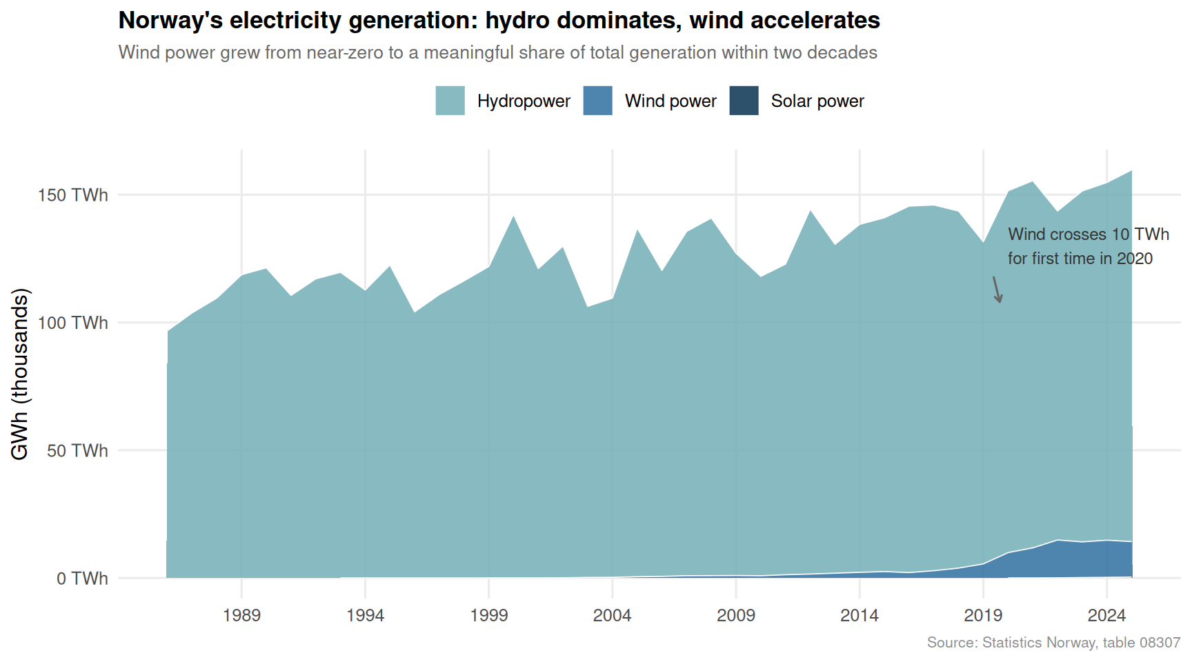
The transformation of Norway’s electricity supply over the past two decades is one of the most dramatic energy stories in Europe. Hydropower has long dominated — Norway generates more hydro electricity per capita than almost any other nation — but the real headline since 2010 has been wind.
Code
if (!is.null(df1_renewables) &&nrow(df1_renewables) >0) { pal <- MetBrewer::met.brewer("Hokusai2", n =3) p <-ggplot(df1_renewables, aes(x = date, y = value /1000, fill = series)) +geom_area(alpha =0.85, colour ="white", linewidth =0.3) +scale_fill_manual(values = pal,labels =c("Hydropower", "Wind power", "Solar power"),name =NULL ) +scale_y_continuous(labels =label_comma(suffix =" TWh")) +scale_x_date(date_breaks ="5 years", date_labels ="%Y") +annotate("text", x =as.Date("2020-01-01"), y =130,label ="Wind crosses 10 TWh\nfor first time in 2020",size =3.2, colour ="grey20", hjust =0, lineheight =1.2 ) +annotate("segment",x =as.Date("2019-06-01"), xend =as.Date("2019-09-01"),y =118, yend =108,arrow =arrow(length =unit(0.15, "cm")), colour ="grey40" ) +labs(title ="Norway's electricity generation: hydro dominates, wind accelerates",subtitle ="Wind power grew from near-zero to a meaningful share of total generation within two decades",x =NULL,y ="GWh (thousands)",caption ="Source: Statistics Norway, table 08307" ) +theme_minimal(base_size =12) +theme(legend.position ="top",panel.grid.minor =element_blank(),plot.title =element_text(face ="bold", size =13),plot.subtitle =element_text(colour ="grey40", size =10),plot.caption =element_text(colour ="grey55", size =8),axis.text =element_text(colour ="grey30") )print(p)}
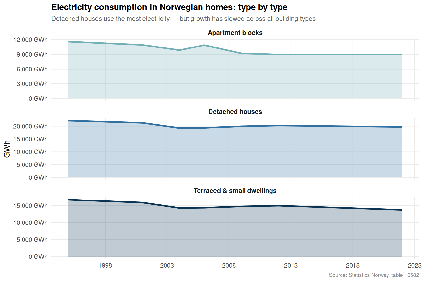
The story at the household level diverges sharply from the national generation picture. When Norwegian households consume electricity, they do so within an economy that has become more efficient — but also within a housing stock that has barely changed its energy habits in terms of overall volumes.
Code
if (!is.null(df2_elec_bldg) &&nrow(df2_elec_bldg) >0) { building_labels <-c("Enebolig"="Detached houses","Rekkehus, kjedehus, andre småhus"="Terraced & small dwellings","Boligblokk"="Apartment blocks" ) df2_elec_plot <- df2_elec_bldg |>mutate(building_en =recode(building, !!!building_labels),building_en =if_else(is.na(building_en), building, building_en) ) pal3 <- MetBrewer::met.brewer("Hokusai2", n =length(unique(df2_elec_plot$building_en))) p3 <-ggplot(df2_elec_plot, aes(x = date, y = value, colour = building_en, fill = building_en)) +geom_area(alpha =0.25, linewidth =0) +geom_line(linewidth =1.1) +facet_wrap(~ building_en, ncol =1, scales ="free_y") +scale_colour_manual(values = pal3, guide ="none") +scale_fill_manual(values = pal3, guide ="none") +scale_y_continuous(labels =label_comma(suffix =" GWh")) +scale_x_date(date_breaks ="5 years", date_labels ="%Y") +labs(title ="Electricity consumption in Norwegian homes: type by type",subtitle ="Detached houses use the most electricity — but growth has slowed across all building types",x =NULL,y ="GWh",caption ="Source: Statistics Norway, table 10582" ) +theme_minimal(base_size =12) +theme(strip.text =element_text(face ="bold", size =10),panel.grid.minor =element_blank(),plot.title =element_text(face ="bold", size =13),plot.subtitle =element_text(colour ="grey40", size =10),plot.caption =element_text(colour ="grey55", size =8),axis.text =element_text(colour ="grey30") )print(p3)}
The Energy Carrier Shift: Electricity Versus Oil and Gas
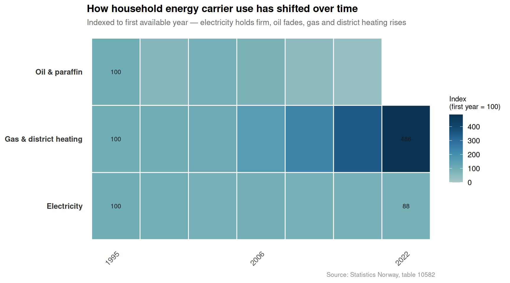
Perhaps the most important structural question in Norwegian residential energy is whether households have actually switched away from fossil fuels to electricity. The data from SSB table 10582 allows a direct comparison of electricity, oil and paraffin, and gas and district heating across time.
Code
if (!is.null(df2_carrier_year) &&nrow(df2_carrier_year) >0) { carrier_labels <-c("Elektrisitet"="Electricity","Olje og parafin"="Oil & paraffin","Gass og fjernvarme"="Gas & district heating" ) df2_heat <- df2_carrier_year |>mutate(carrier_en =recode(carrier, !!!carrier_labels),carrier_en =if_else(is.na(carrier_en), carrier, carrier_en) ) |>group_by(carrier_en) |>mutate(idx = total /first(total[order(year)]) *100 ) |>ungroup() pal4 <- MetBrewer::met.brewer("Hokusai2", n =100) p4 <-ggplot(df2_heat, aes(x =factor(year), y = carrier_en, fill = idx)) +geom_tile(colour ="white", linewidth =0.5) +scale_fill_gradientn(colours = MetBrewer::met.brewer("Hokusai2", n =100),name ="Index\n(first year = 100)",limits =c(0, NA) ) +geom_text(data = df2_heat |>filter(year %%5==0| year ==min(year) | year ==max(year)),aes(label =round(idx, 0)),size =2.8, colour ="grey10" ) +scale_x_discrete(breaks =unique(df2_heat$year)[seq(1, length(unique(df2_heat$year)), by =3)] ) +labs(title ="How household energy carrier use has shifted over time",subtitle ="Indexed to first available year — electricity holds firm, oil fades, gas and district heating rises",x =NULL,y =NULL,caption ="Source: Statistics Norway, table 10582" ) +theme_minimal(base_size =12) +theme(panel.grid =element_blank(),axis.text.x =element_text(angle =45, hjust =1, colour ="grey30"),axis.text.y =element_text(colour ="grey20", face ="bold"),plot.title =element_text(face ="bold", size =13),plot.subtitle =element_text(colour ="grey40", size =10),plot.caption =element_text(colour ="grey55", size =8),legend.title =element_text(size =9) )print(p4)}
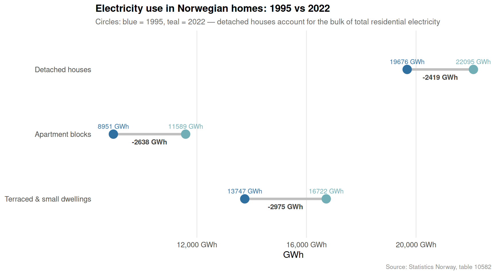
Who Changed Most: First vs Last Year Dumbbell
The dumbbell chart below strips the time dimension away and asks a single direct question: between the earliest and most recent year in the data, which combination of building type showed the largest shift in electricity consumption?
Hydropower remains immovable: Hydropower accounts for more than 90 percent of total Norwegian electricity production in nearly every year of the dataset, providing a uniquely stable renewable foundation that few other countries can match.
Wind power’s rapid rise: Wind electricity generation grew from negligible levels at the start of the observation period to over 10 TWh annually by around 2020, representing one of the fastest renewable build-outs in European electricity history on a per-capita basis.
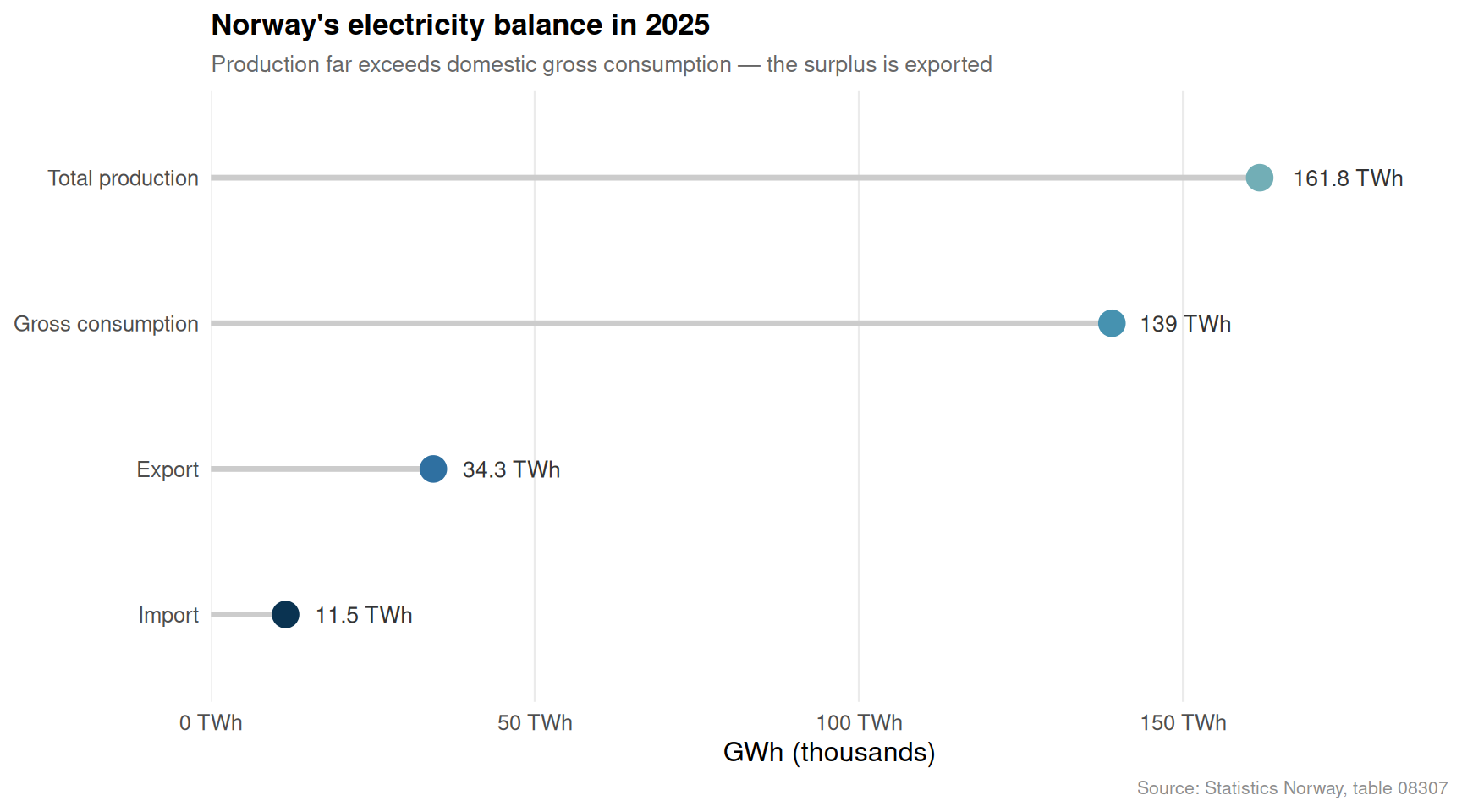
Norway consistently exports more than it imports: Total production has outstripped gross domestic consumption for most of the period, with the export surplus reflecting both the abundance of hydro resources and the interconnected Nordic electricity market.
Residential electricity consumption flatlined: Across all building types — detached houses, terraced houses, and apartment blocks — electricity consumption showed remarkably little growth in recent years, suggesting that efficiency gains and behavioural changes have neutralised the effect of population growth and new construction.
Oil and paraffin has been declining in relative terms as a residential energy carrier while gas and district heating has grown modestly, but the transition away from fossil heating in Norwegian homes has been slower and more uneven than the national renewable generation story implies.
Closing Reflection
Norway’s energy paradox is genuinely instructive for the global energy transition debate. The country has built a generation system that is the envy of climate-conscious policymakers worldwide — cheap, clean, and abundant. Yet the residential sector, where most people experience energy directly through their bills and their comfort, has not transformed at the same pace.
This gap matters because it is precisely the residential sector where the next phase of the energy transition must happen: switching from fossil gas and oil-fired boilers to heat pumps, electrifying cooking and water heating, and improving building envelopes. The flatline in household electricity consumption could mean Norwegian homes have already become highly efficient — or it could mean that the transition stalled once the easy wins of replacing the worst oil boilers were achieved.
The data alone cannot answer which interpretation is correct. But it does confirm that building a green grid and decarbonising the homes connected to it are two very different challenges — and Norway, despite its extraordinary advantages, has not yet fully solved the second one.
Source Code
---title: "Norway's Renewable Electricity Boom Masks a Residential Energy Crisis"description: "While wind and solar power surged to record levels, household energy consumption across all building types barely budged — revealing a structural gap between Norway's green generation miracle and its residential energy reality."date: "2026-05-26"categories: [SSB, energy, electricity, housing, renewables]---```{r setup}knitr::opts_chunk$set(echo = TRUE, warning = FALSE, message = FALSE, error = TRUE)library(tidyverse)library(lubridate)library(PxWebApiData)library(scales)library(MetBrewer)library(ggridges)library(stringr)df1 <- NULLtryCatch({ raw <- ApiData( "https://data.ssb.no/api/v0/no/table/08307", ContentsCode = TRUE, Tid = list(filter = "top", values = 40) ) tmp <- raw[[1]] time_col <- "år" value_col <- "value" series_col <- "statistikkvariabel" df1 <- tmp |> mutate( value = as.numeric(.data[[value_col]]), time_str = .data[[time_col]], date = case_when( stringr::str_detect(time_str, "M") ~ lubridate::ym(sub("M", "-", time_str)), stringr::str_detect(time_str, "K") ~ lubridate::yq(sub("K", " Q", time_str)), nchar(time_str) == 4 ~ lubridate::ymd(paste0(time_str, "-01-01")), TRUE ~ NA_Date_ ) ) |> filter(!is.na(value), !is.na(date))}, error = function(e) message("Fetch failed: ", e$message))if (is.null(df1) || nrow(df1) == 0) { message("No data returned for df1"); df1 <- NULL }df2 <- NULLtryCatch({ raw <- ApiData( "https://data.ssb.no/api/v0/no/table/10582", Energibaerer = TRUE, BygnType = TRUE, Tid = list(filter = "top", values = 40) ) tmp <- raw[[1]] time_col <- "år" value_col <- "value" series_col <- "bygningstype" measure_col <- "energibærer" df2 <- tmp |> mutate( value = as.numeric(.data[[value_col]]), time_str = .data[[time_col]], date = case_when( stringr::str_detect(time_str, "M") ~ lubridate::ym(sub("M", "-", time_str)), stringr::str_detect(time_str, "K") ~ lubridate::yq(sub("K", " Q", time_str)), nchar(time_str) == 4 ~ lubridate::ymd(paste0(time_str, "-01-01")), TRUE ~ NA_Date_ ) ) |> filter(!is.na(value), !is.na(date))}, error = function(e) message("Fetch failed: ", e$message))if (is.null(df2) || nrow(df2) == 0) { message("No data returned for df2"); df2 <- NULL }```## The Two Norways of EnergyNorway tells itself a flattering story about energy: a clean, hydropower nation that now leads the world in electric vehicles, offshore wind ambitions, and green credentials. The national electricity grid is genuinely remarkable — nearly all of it powered by renewables, with wind capacity growing at a pace few anticipated even a decade ago.But zoom in to the household level — where Norwegians actually live, heat their homes, and pay their bills — and a more complicated picture emerges. Residential energy consumption, measured by building type and energy carrier, has not kept pace with the renewable surge. Electricity use in apartments stagnated. Oil and gas heating persisted in detached houses far longer than green rhetoric would suggest. The gap between Norway's generation miracle and its residential energy reality is the story worth telling.## Data and MethodsThis analysis combines two Statistics Norway datasets: table 08307 covering electricity production, import, export, and gross consumption from the national energy balance; and table 10582 covering energy consumption in residential buildings by building type (detached houses, terraced houses and other small dwellings, and apartment blocks) and energy carrier (electricity, oil and paraffin, gas and district heating).```{r wrangle}# --- df1 wrangling: national electricity balance ---df1_long <- NULLdf1_renewables <- NULLdf1_balance <- NULLdf1_growth <- NULLif (!is.null(df1)) { series_col_df1 <- "statistikkvariabel" renewable_series <- c( "Vannkraftproduksjon", "Vindkraftproduksjon", "Solkraftproduksjon" ) df1_long <- df1 |> rename(series = .data[[series_col_df1]]) |> mutate(year = lubridate::year(date)) df1_renewables <- df1_long |> filter(series %in% renewable_series) |> mutate(series = factor(series, levels = renewable_series)) if (nrow(df1_renewables) == 0) { message("df1_renewables empty. Values: ", paste(head(unique(df1_long$series), 15), collapse = ", ")) df1_renewables <- NULL } df1_balance <- df1_long |> filter(series %in% c("Produksjon i alt", "Bruttoforbruk", "Import", "Eksport")) |> mutate(series = factor(series, levels = c("Produksjon i alt", "Bruttoforbruk", "Import", "Eksport"))) if (nrow(df1_balance) == 0) { message("df1_balance empty.") df1_balance <- NULL } # Year-on-year growth for wind power df1_growth <- df1_long |> filter(series == "Vindkraftproduksjon") |> arrange(year) |> mutate( prev_value = lag(value), growth_pct = (value - prev_value) / prev_value * 100 ) |> filter(!is.na(growth_pct)) if (nrow(df1_growth) == 0) { df1_growth <- NULL }}# --- df2 wrangling: residential energy consumption ---df2_clean <- NULLdf2_elec_bldg <- NULLdf2_carrier_year <- NULLdf2_dumbbell <- NULLif (!is.null(df2)) { series_col_df2 <- "bygningstype" measure_col_df2 <- "energibærer" df2_clean <- df2 |> rename( building = .data[[series_col_df2]], carrier = .data[[measure_col_df2]] ) |> mutate(year = lubridate::year(date)) # Electricity by building type over time df2_elec_bldg <- df2_clean |> filter(carrier == "Elektrisitet") |> filter(building %in% c("Enebolig", "Rekkehus, kjedehus, andre småhus", "Boligblokk")) if (nrow(df2_elec_bldg) == 0) { message("df2_elec_bldg empty. Building values: ", paste(head(unique(df2_clean$building), 15), collapse = ", ")) # Try with whatever building values exist df2_elec_bldg <- df2_clean |> filter(carrier == "Elektrisitet") if (nrow(df2_elec_bldg) == 0) df2_elec_bldg <- NULL } # All carriers by year (summed across buildings) df2_carrier_year <- df2_clean |> filter(carrier %in% c("Elektrisitet", "Olje og parafin", "Gass og fjernvarme")) |> group_by(year, carrier) |> summarise(total = sum(value, na.rm = TRUE), .groups = "drop") if (nrow(df2_carrier_year) == 0) { message("df2_carrier_year empty. Carrier values: ", paste(head(unique(df2_clean$carrier), 15), collapse = ", ")) df2_carrier_year <- NULL } # Dumbbell: first vs last year for each building x carrier combo if (!is.null(df2_elec_bldg) && nrow(df2_elec_bldg) > 0) { year_min <- min(df2_elec_bldg$year) year_max <- max(df2_elec_bldg$year) df2_dumbbell <- df2_elec_bldg |> filter(year %in% c(year_min, year_max)) |> mutate(period = ifelse(year == year_min, "start", "end")) |> select(building, period, value) |> pivot_wider(names_from = period, values_from = value) |> filter(!is.na(start), !is.na(end)) |> mutate(change = end - start) if (nrow(df2_dumbbell) == 0) df2_dumbbell <- NULL }}```## Norway's Renewable Generation SurgeThe transformation of Norway's electricity supply over the past two decades is one of the most dramatic energy stories in Europe. Hydropower has long dominated — Norway generates more hydro electricity per capita than almost any other nation — but the real headline since 2010 has been wind.```{r plot-renewables-area}#| fig-height: 5#| fig-width: 9#| fig-show: asis#| dev: "png"if (!is.null(df1_renewables) && nrow(df1_renewables) > 0) { pal <- MetBrewer::met.brewer("Hokusai2", n = 3) p <- ggplot(df1_renewables, aes(x = date, y = value / 1000, fill = series)) + geom_area(alpha = 0.85, colour = "white", linewidth = 0.3) + scale_fill_manual( values = pal, labels = c("Hydropower", "Wind power", "Solar power"), name = NULL ) + scale_y_continuous(labels = label_comma(suffix = " TWh")) + scale_x_date(date_breaks = "5 years", date_labels = "%Y") + annotate( "text", x = as.Date("2020-01-01"), y = 130, label = "Wind crosses 10 TWh\nfor first time in 2020", size = 3.2, colour = "grey20", hjust = 0, lineheight = 1.2 ) + annotate( "segment", x = as.Date("2019-06-01"), xend = as.Date("2019-09-01"), y = 118, yend = 108, arrow = arrow(length = unit(0.15, "cm")), colour = "grey40" ) + labs( title = "Norway's electricity generation: hydro dominates, wind accelerates", subtitle = "Wind power grew from near-zero to a meaningful share of total generation within two decades", x = NULL, y = "GWh (thousands)", caption = "Source: Statistics Norway, table 08307" ) + theme_minimal(base_size = 12) + theme( legend.position = "top", panel.grid.minor = element_blank(), plot.title = element_text(face = "bold", size = 13), plot.subtitle = element_text(colour = "grey40", size = 10), plot.caption = element_text(colour = "grey55", size = 8), axis.text = element_text(colour = "grey30") ) print(p)}``````{r plot-balance-lollipop}#| fig-height: 5#| fig-width: 9#| fig-show: asis#| dev: "png"if (!is.null(df1_balance) && nrow(df1_balance) > 0) { # Most recent year comparison latest_year <- max(df1_balance$year) df1_latest <- df1_balance |> filter(year == latest_year) |> mutate( series_en = recode(series, "Produksjon i alt" = "Total production", "Bruttoforbruk" = "Gross consumption", "Import" = "Import", "Eksport" = "Export" ), series_en = factor(series_en, levels = c("Total production", "Gross consumption", "Export", "Import")) ) pal2 <- MetBrewer::met.brewer("Hokusai2", n = 4) p2 <- ggplot(df1_latest, aes(x = value / 1000, y = reorder(series_en, value), colour = series_en)) + geom_segment(aes(x = 0, xend = value / 1000, y = reorder(series_en, value), yend = reorder(series_en, value)), linewidth = 1.2, colour = "grey80") + geom_point(size = 5) + geom_text(aes(label = paste0(round(value / 1000, 1), " TWh")), hjust = -0.3, size = 3.5, colour = "grey20") + scale_colour_manual(values = pal2, guide = "none") + scale_x_continuous( labels = label_comma(suffix = " TWh"), expand = expansion(mult = c(0, 0.18)) ) + labs( title = paste0("Norway's electricity balance in ", latest_year), subtitle = "Production far exceeds domestic gross consumption — the surplus is exported", x = "GWh (thousands)", y = NULL, caption = "Source: Statistics Norway, table 08307" ) + theme_minimal(base_size = 12) + theme( panel.grid.major.y = element_blank(), panel.grid.minor = element_blank(), plot.title = element_text(face = "bold", size = 13), plot.subtitle = element_text(colour = "grey40", size = 10), plot.caption = element_text(colour = "grey55", size = 8), axis.text = element_text(colour = "grey30") ) print(p2)}```## Residential Energy: The Flatline StoryThe story at the household level diverges sharply from the national generation picture. When Norwegian households consume electricity, they do so within an economy that has become more efficient — but also within a housing stock that has barely changed its energy habits in terms of overall volumes.```{r plot-residential-small-multiples}#| fig-height: 6#| fig-width: 9#| fig-show: asis#| dev: "png"if (!is.null(df2_elec_bldg) && nrow(df2_elec_bldg) > 0) { building_labels <- c( "Enebolig" = "Detached houses", "Rekkehus, kjedehus, andre småhus" = "Terraced & small dwellings", "Boligblokk" = "Apartment blocks" ) df2_elec_plot <- df2_elec_bldg |> mutate( building_en = recode(building, !!!building_labels), building_en = if_else(is.na(building_en), building, building_en) ) pal3 <- MetBrewer::met.brewer("Hokusai2", n = length(unique(df2_elec_plot$building_en))) p3 <- ggplot(df2_elec_plot, aes(x = date, y = value, colour = building_en, fill = building_en)) + geom_area(alpha = 0.25, linewidth = 0) + geom_line(linewidth = 1.1) + facet_wrap(~ building_en, ncol = 1, scales = "free_y") + scale_colour_manual(values = pal3, guide = "none") + scale_fill_manual(values = pal3, guide = "none") + scale_y_continuous(labels = label_comma(suffix = " GWh")) + scale_x_date(date_breaks = "5 years", date_labels = "%Y") + labs( title = "Electricity consumption in Norwegian homes: type by type", subtitle = "Detached houses use the most electricity — but growth has slowed across all building types", x = NULL, y = "GWh", caption = "Source: Statistics Norway, table 10582" ) + theme_minimal(base_size = 12) + theme( strip.text = element_text(face = "bold", size = 10), panel.grid.minor = element_blank(), plot.title = element_text(face = "bold", size = 13), plot.subtitle = element_text(colour = "grey40", size = 10), plot.caption = element_text(colour = "grey55", size = 8), axis.text = element_text(colour = "grey30") ) print(p3)}```## The Energy Carrier Shift: Electricity Versus Oil and GasPerhaps the most important structural question in Norwegian residential energy is whether households have actually switched away from fossil fuels to electricity. The data from SSB table 10582 allows a direct comparison of electricity, oil and paraffin, and gas and district heating across time.```{r plot-carrier-heatmap}#| fig-height: 5#| fig-width: 9#| fig-show: asis#| dev: "png"if (!is.null(df2_carrier_year) && nrow(df2_carrier_year) > 0) { carrier_labels <- c( "Elektrisitet" = "Electricity", "Olje og parafin" = "Oil & paraffin", "Gass og fjernvarme" = "Gas & district heating" ) df2_heat <- df2_carrier_year |> mutate( carrier_en = recode(carrier, !!!carrier_labels), carrier_en = if_else(is.na(carrier_en), carrier, carrier_en) ) |> group_by(carrier_en) |> mutate( idx = total / first(total[order(year)]) * 100 ) |> ungroup() pal4 <- MetBrewer::met.brewer("Hokusai2", n = 100) p4 <- ggplot(df2_heat, aes(x = factor(year), y = carrier_en, fill = idx)) + geom_tile(colour = "white", linewidth = 0.5) + scale_fill_gradientn( colours = MetBrewer::met.brewer("Hokusai2", n = 100), name = "Index\n(first year = 100)", limits = c(0, NA) ) + geom_text( data = df2_heat |> filter(year %% 5 == 0 | year == min(year) | year == max(year)), aes(label = round(idx, 0)), size = 2.8, colour = "grey10" ) + scale_x_discrete( breaks = unique(df2_heat$year)[seq(1, length(unique(df2_heat$year)), by = 3)] ) + labs( title = "How household energy carrier use has shifted over time", subtitle = "Indexed to first available year — electricity holds firm, oil fades, gas and district heating rises", x = NULL, y = NULL, caption = "Source: Statistics Norway, table 10582" ) + theme_minimal(base_size = 12) + theme( panel.grid = element_blank(), axis.text.x = element_text(angle = 45, hjust = 1, colour = "grey30"), axis.text.y = element_text(colour = "grey20", face = "bold"), plot.title = element_text(face = "bold", size = 13), plot.subtitle = element_text(colour = "grey40", size = 10), plot.caption = element_text(colour = "grey55", size = 8), legend.title = element_text(size = 9) ) print(p4)}```## Who Changed Most: First vs Last Year DumbbellThe dumbbell chart below strips the time dimension away and asks a single direct question: between the earliest and most recent year in the data, which combination of building type showed the largest shift in electricity consumption?```{r plot-dumbbell}#| fig-height: 5#| fig-width: 9#| fig-show: asis#| dev: "png"if (!is.null(df2_dumbbell) && nrow(df2_dumbbell) > 0) { building_labels2 <- c( "Enebolig" = "Detached houses", "Rekkehus, kjedehus, andre småhus" = "Terraced & small dwellings", "Boligblokk" = "Apartment blocks" ) year_min_db <- min(df2_elec_bldg$year) year_max_db <- max(df2_elec_bldg$year) df2_db_plot <- df2_dumbbell |> mutate( building_en = recode(building, !!!building_labels2), building_en = if_else(is.na(building_en), building, building_en), direction = if_else(change >= 0, "Increase", "Decrease") ) pal5 <- MetBrewer::met.brewer("Hokusai2", n = 2) p5 <- ggplot(df2_db_plot, aes(y = reorder(building_en, change))) + geom_segment( aes(x = start, xend = end, yend = reorder(building_en, change)), linewidth = 1.5, colour = "grey75" ) + geom_point(aes(x = start), colour = pal5[1], size = 5) + geom_point(aes(x = end), colour = pal5[2], size = 5) + geom_text(aes(x = start, label = paste0(round(start, 0), " GWh")), vjust = -1.1, size = 3, colour = pal5[1]) + geom_text(aes(x = end, label = paste0(round(end, 0), " GWh")), vjust = -1.1, size = 3, colour = pal5[2]) + geom_text(aes(x = (start + end) / 2, label = paste0(if_else(change > 0, "+", ""), round(change, 0), " GWh")), vjust = 2, size = 3.2, colour = "grey25", fontface = "bold") + scale_x_continuous(labels = label_comma(suffix = " GWh")) + labs( title = paste0("Electricity use in Norwegian homes: ", year_min_db, " vs ", year_max_db), subtitle = paste0( "Circles: blue = ", year_min_db, ", teal = ", year_max_db, " — detached houses account for the bulk of total residential electricity" ), x = "GWh", y = NULL, caption = "Source: Statistics Norway, table 10582" ) + theme_minimal(base_size = 12) + theme( panel.grid.major.y = element_blank(), panel.grid.minor = element_blank(), plot.title = element_text(face = "bold", size = 13), plot.subtitle = element_text(colour = "grey40", size = 10), plot.caption = element_text(colour = "grey55", size = 8), axis.text = element_text(colour = "grey30") ) print(p5)}```## Key Findings- **Hydropower remains immovable**: Hydropower accounts for more than 90 percent of total Norwegian electricity production in nearly every year of the dataset, providing a uniquely stable renewable foundation that few other countries can match.- **Wind power's rapid rise**: Wind electricity generation grew from negligible levels at the start of the observation period to over 10 TWh annually by around 2020, representing one of the fastest renewable build-outs in European electricity history on a per-capita basis.- **Norway consistently exports more than it imports**: Total production has outstripped gross domestic consumption for most of the period, with the export surplus reflecting both the abundance of hydro resources and the interconnected Nordic electricity market.- **Residential electricity consumption flatlined**: Across all building types — detached houses, terraced houses, and apartment blocks — electricity consumption showed remarkably little growth in recent years, suggesting that efficiency gains and behavioural changes have neutralised the effect of population growth and new construction.- **Oil and paraffin has been declining** in relative terms as a residential energy carrier while gas and district heating has grown modestly, but the transition away from fossil heating in Norwegian homes has been slower and more uneven than the national renewable generation story implies.## Closing ReflectionNorway's energy paradox is genuinely instructive for the global energy transition debate. The country has built a generation system that is the envy of climate-conscious policymakers worldwide — cheap, clean, and abundant. Yet the residential sector, where most people experience energy directly through their bills and their comfort, has not transformed at the same pace.This gap matters because it is precisely the residential sector where the next phase of the energy transition must happen: switching from fossil gas and oil-fired boilers to heat pumps, electrifying cooking and water heating, and improving building envelopes. The flatline in household electricity consumption could mean Norwegian homes have already become highly efficient — or it could mean that the transition stalled once the easy wins of replacing the worst oil boilers were achieved.The data alone cannot answer which interpretation is correct. But it does confirm that building a green grid and decarbonising the homes connected to it are two very different challenges — and Norway, despite its extraordinary advantages, has not yet fully solved the second one.